Article

Molecular Toxicity Virtual Screening Applying a Quantized Computational SNN-Based Framework

1
Department of Health Sciences, Center on Autoimmune and Allergic Diseases CAAD, Università del Piemonte Orientale, 28100 Novara, Italy
2
Enginsoft SpA, 35129 Padua, Italy
*
Author to whom correspondence should be addressed.
Molecules 2023, 28(3), 1342; https://doi.org/10.3390/molecules28031342
Submission received: 30 December 2022 / Revised: 27 January 2023 / Accepted: 29 January 2023 / Published: 31 January 2023
(This article belongs to the Special Issue Shaping Medicinal Chemistry for the New Decade)

Abstract

:
Spiking neural networks are biologically inspired machine learning algorithms attracting researchers’ attention for their applicability to alternative energy-efficient hardware other than traditional computers. In the current work, spiking neural networks have been tested in a quantitative structure–activity analysis targeting the toxicity of molecules. Multiple public-domain databases of compounds have been evaluated with spiking neural networks, achieving accuracies compatible with high-quality frameworks presented in the previous literature. The numerical experiments also included an analysis of hyperparameters and tested the spiking neural networks on molecular fingerprints of different lengths. Proposing alternatives to traditional software and hardware for time- and resource-consuming tasks, such as those found in chemoinformatics, may open the door to new research and improvements in the field.

1. Introduction

Machine learning (i.e., ML) techniques provide data-driven tools to screen small molecules for quantitative structure–activity or property relationships (i.e., QSAR/QSPR), contributing to the preliminary selection of candidate compounds that will be validated experimentally by in vitro or in vivo assays [1]. ML QSAR models establish a connection between the structure of a molecule and its activity by regression if the property under investigation is continuous or by classification if the biological outcome is categorical [2]. Prioritizing the most suitable molecules for the goals of an experiment by virtual screening brings advantages in terms of time and resource-saving. Moreover, it can be carried out in a high-throughput fashion [3]. Machine learning algorithms previously tested on bioactivity data prediction included classic methodologies such as random forests [4,5,6,7], support vector machines [8,9,10], or k-nearest neighbors [11,12]; in addition, deep neural networks (i.e., NNs) were also employed due to their performance in examining complex libraries of compounds [13]. Spiking neural networks (i.e., SNNs) are different machine learning systems built around the concept of simulating biological processes by replacing the perceptron [14] with neuronal models borrowed from computational biology [15]. In recent years, the growing interest of the scientific community in these innovative networks led to the development of specific event-driven hardware to accomplish brain-inspired computations [16]. Pairing software based on spiking neural networks to neuromorphic computers, it could be possible to achieve low-power computations [17]. Together with quantum computing, neuromorphic platforms are alternatives to the standard clock-based hardware for bypassing the increasing demand of computational resources required by deep learning algorithms [18].
In ML QSAR, relating a molecule to a property requires encoding the molecule’s structural information into a learnable representation. After encoding, the molecular formula could be utilized in specialized software [19] or libraries [20] to extract descriptors acting as input features for ML models. These programs accept compounds portrayed as alphanumeric strings called simplified molecular-input line-entry systems (i.e., SMILES). However, recently several authors feed SMILES directly to their encoder–decoder models for property forecasting [21,22]: these models exploit the internal NN representations as latent features. Alternatively, the molecular structure could be represented in the form of graphs, non-Euclidean datatypes consisting of nodes and edges [23]; in that case, applying SMILES as starting data is beneficial because decoding the molecular graph directly may increase the complexity of the model [24]. Although implementing graph-based NN for property prediction is a popular choice still, a few problems affect this methodology: underfitting the train set [25], lack of performance on small datasets [26], over-smoothing [27], information loss while encoding the graph to a vector [28], and inability to preserve long-range node dependencies [29]. Due to these limitations, the classic ML model applied to molecular fingerprints still retains its validity, achieving remarkable results in QSAR studies [30,31,32]. Several of these ML protocols for virtual screening employ molecular fingerprints (i.e., MFs) as inputs rather than SMILES, substituting ASCII characters with sparse binary vectors collecting compounds’ features [33]. The MFs are sequences of bits illustrating the presence or lack of a specific molecular substructure; the length of the MFs is variable, ranging from 166 bits of the Molecular ACCess System (i.e., MAACS) [34] to 1024 of Daylight Chemical Information Systems [35] or 2048 bits using Morgan’s extended-connectivity fingerprints [36].
The current study aims to employ SNN for toxicity prediction using datasets of compounds converted into MAACS fingerprints. The choice of fingerprints as input data for the SNN is derived from the observation according to which binary vectors are the natural input of SNNs. Indeed, SNNs receive incoming information encoded as bit sequences that simulate neuronal spike trains [37]. The mechanism of the neurons constituting an SNN is similar to the activity in human neurons: the membrane potential is sensitive to over-threshold stimuli, causing modulations of trans-membrane ionic currents and the consequent passage of information to the following cell. The crucial aspect of SNNs compared to traditional NNs, is that not all information is transmitted to the next layer at every cycle, but only after certain conditions measured in terms of membrane voltages are met. In chemoinformatics, the application of SNNs is a novelty and this work may be the first attempt to promote SNN in QSAR toxicological investigations. The current work will test SNNs extensively in large databases of molecules with different characteristics; special attention will be paid to SNN parameter tuning, a practical aspect usually reported as challenging to handle [38]. This study will further relate chemoinformatics QSAR modeling to the novel field of neuroscience-inspired artificial intelligence [39].

2. Results

The results include the single dataset assessment by the SNNs (Section 2.1), SNN hyperparameter report for the best models (Section 2.2), and meta-analysis with the previous literature on the same data (Section 2.3). In Section 2.4, the SNN architectures studied for MAACS MFs were evaluated on more advanced MFs to judge the scalability of SNNs when providing inputs of different lengths.

2.1. Classification Outcomes

The results of the numerical experiments applying SNNs on each dataset for medicinal chemistry were reported in the following tables. Only the top five outcomes were included, with accuracy values reported as mean and standard deviation (i.e., Std) of the CV repetitions.

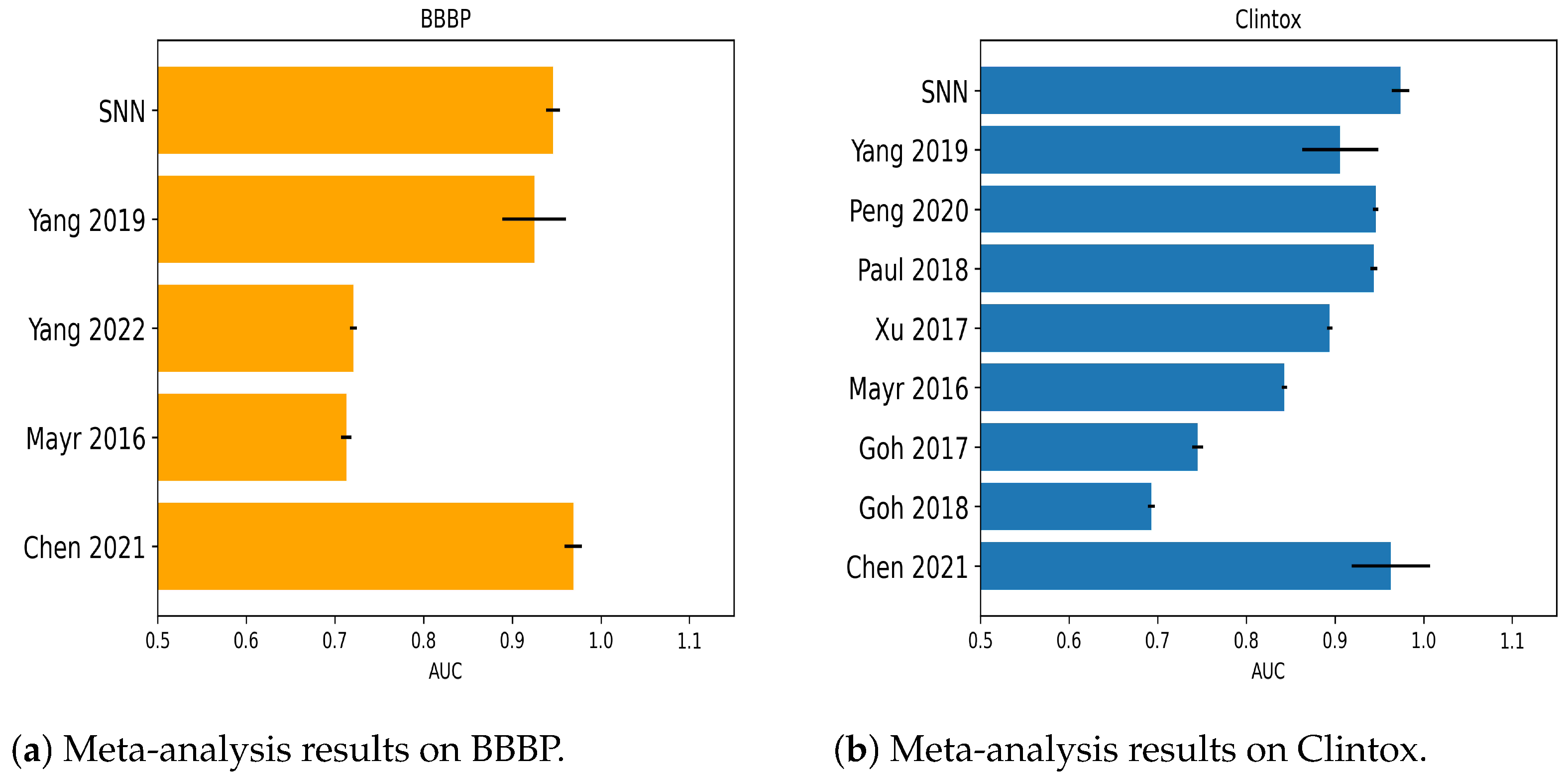
2.1.1. Numerical Experiments on Clintox

The toxicity in clinical trials found by the U.S. Food and Drug Administration is the binary outcome (FDA-approved or not) of the Clintox benchmark. Classification outcomes of SNNs were collected in Table 1.

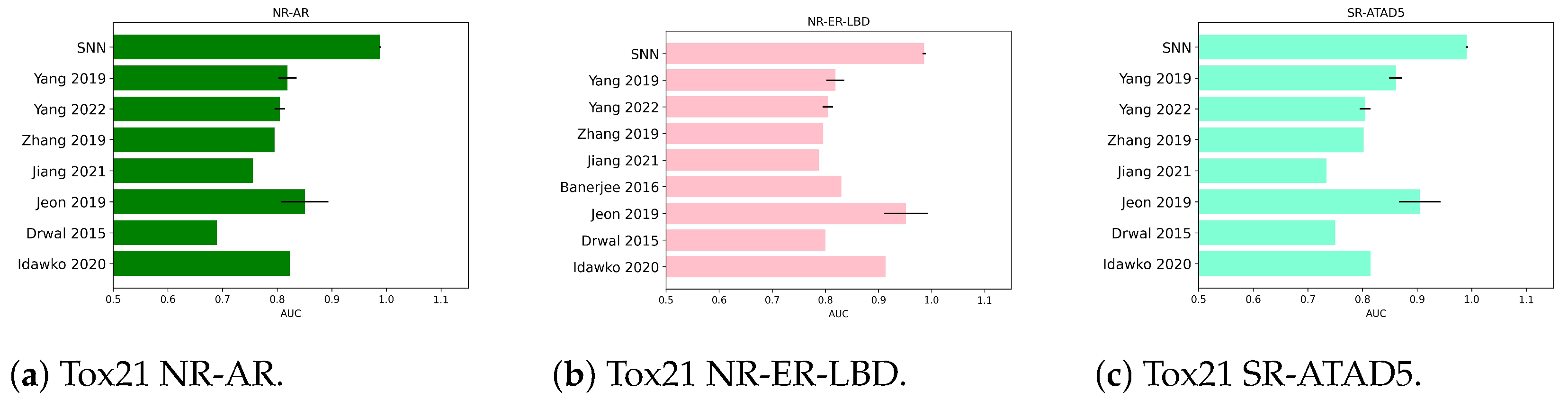
2.1.2. Numerical Experiments on Tox21 NR-AR

The Tox21 dataset contains several measurements regarding toxicity by in vitro high-throughput screening. The NR-AR measures the anti-androgenic toxicity estimated in nipple retention. The SNN performance on this task is portrayed in Table 2.

2.1.3. Numerical Experiments on Tox21 NR-ER-LBD

From Tox 21, the NR-ER-LBD variable determines the estrogen receptor nipple receptor binding site for transcriptional activity. It is an indicator of organ toxicity through the pathway for etonogestrel, a medication for birth control in women. The outcomes of the numerical experiments with SNN are delineated in Table 3.

2.1.4. Numerical Experiments on Tox21 SR-ATAD5

In Tox21, the measurement SR-ATAD5 is not a toxicity target as a nuclear receptor but a quantity connected with the stress response pathway. It quantifies the genotoxicity captured by the ATAD5 signaling pathway as part of the stress response panel activated when a cell detects DNA damage. Classification outcomes from SNNs could be found in Table 4.

2.1.5. Numerical Experiments on TOXCAST TR-LUC-GH3-Ant

The dataset TOXCAST was created by in vitro high-throughput screening and included several effects on biochemical endpoints, cellular processes, and phenotypes in humans or animals. The SNN investigation focused on the thyroid function mediated by TR genes regulated by the GH3 cell line. The TR-interacting compounds disrupt thyroid homeostasis. The balanced accuracies of the top-performing SNNs were gathered in Table 5.

2.1.6. Numerical Experiments on BBBP

The blood–brain barrier plays an essential role in protecting the nervous system and maintaining the microenvironment of the brain. Drugs targeting the central nervous system should be able to penetrate the blood–brain barrier. The SNN results on the compounds of the BBBP benchmark in detecting permeability were included in Table 6.

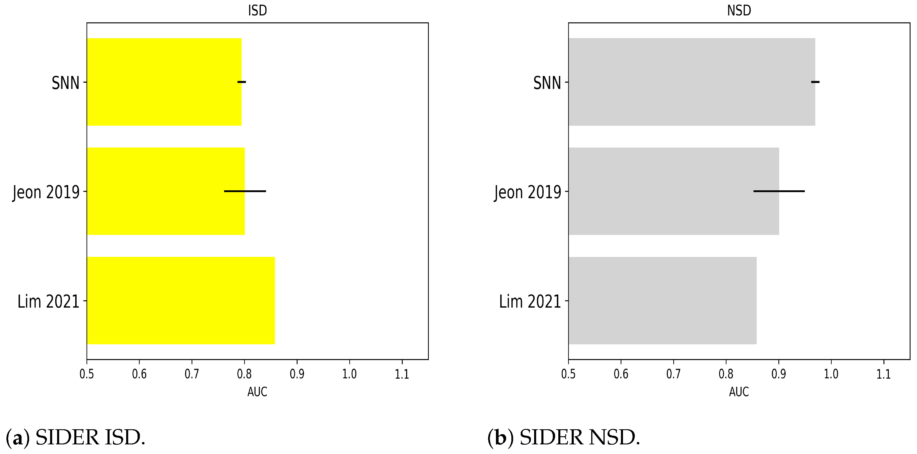
2.1.7. Numerical Experiments on SIDER ISD

The Side Effect Resource dataset describes marketed drugs and their adverse reaction to specific human body systems. Those affecting the immune system were analyzed in the ISD screened by SNNs. Outcomes are summarized in Table 7.

2.1.8. Numerical Experiments on SIDER NSD

Commercial drugs that affect the nervous system as side effects are present in the NSD part of the SIDER dataset. The SNNs evaluated for this type of disorder reached accuracies shown in Table 8.

2.2. Hyperparameters Evaluation

The SNN hyperparameters of the best SNN models were reported in Table 9. The models generally had a membrane decay rate between 0.8 and 0.95 and a surrogate gradient of 50 or 75. All the best architectures comprised 1000 neurons, except one with 1200.
To enhance the comparison with previous articles in Section 2.3, the SNN outcomes on the test set have been recomputed in terms of AUC and added to Table 9. The validation set accuracies were included in Appendix A Table A1.

2.3. Meta-Analysis

This section is subdivided into two parts: an initial report of previous works running classification on MFs as inputs (Section 2.3.1), and a latter part (Section 2.3.2), including manuscripts adopting different frameworks for in silico toxicity prediction. Section 2.3.3 summarizes in graphical format the comparisons between SNNs and other methodologies from the previous literature.

2.3.1. Previous Literature on Virtual Screenings from MFs

The first comparison was conducted over the results presented by [40] using a random forest (i.e., RF) and Morgan MFs on BBBP (0.909 ± 0.028 AUC), Tox21 (0.819 ± 0.017), SIDER (0.687 ± 0.014), and ClinTox (0.759 ± 0.060). In [41], the authors evaluated MAACS fingerprints over the Tox21 dataset achieving an AUC of 0.805 ± 0.01, an AUC of 0.721 ± 0.004 for BBBP, and an AUC equal to 0.797 ± 0.151 for Clintox, applying an ensemble of decision trees over 5-fold cross-validation. Another paper [42] focused on the Tox21 dataset reporting the outcomes of the in silico toxicity evaluation by five classifiers on Morgan fingerprints: the LightGBM overperformed other classifiers, reaching an AUC of 0.795 on the test set (standard deviation was not reported) for NR-AR. Other classifiers included in the study were random forest (0.777), support vector machines with radial basis function (0.784), extreme gradient boosting (0.777), and a deep neural network with three hidden layers coupled with Adam as optimizer (0.787). This latter work shares with the current investigation the choice of nested CV as a practical approach to keep separated HP tuning and evaluation of the estimators. On NR-ER-LBD, LightGBM reached 0.796, whereas on SR-ATAD5, it fulfilled 0.802 AUC. In [43], the authors analyzed the Tox21 dataset (the 10k version) using multiscale weighted colored graph MFs and compared the results of different classifiers to MAACS MF. The outcomes for the gradient boosting decision tree on MAACS for NR-AR was0.756 AUC, for NR-ER-LBD was 0.788, and for SR-ATAD5 was 0.734. Another work testing several classifiers on Tox21 was [44], reporting on NR-ER-LBD 0.83 AUC employing RF on MAACS MFs, 0.73 AUC with naive Bayes, and 0.78 AUC with probabilistic NN. The authors of [45] generated Morgan MFs for SIDER, BBBP, and Tox21 datasets evaluating the benchmarks by convolutional NN (Table A2). They applied the convolutional NN on single learning tasks for each dataset (similar to what was performed during the current investigation on SNN), or the same NN applied in multitask learning, as in [46], obtaining better results. The authors of [47] evaluated different MFs on Tox21 data with a naïve Bayes classifier, reaching 0.7664 and 0.772 AUC with MAACS MFs for active or inactive compounds on NR-ER-LBD, respectively. The results were raised to 0.8 on the test set combining MFs to a similarity score. The authors used the same scheme to obtain 0.69 on NR-AR and 0.75 on SR-ATAD5. From MAACS MFs and working with an RF classifier, the researchers in [48] reported 0.8151 AUC on SR-ATAD5, adopting a synthetic data generation scheme to solve the class instances’ imbalance. The same group obtained 0.8232 without imbalance adjustments on NR-AR and 0.9133 on NR-ER-LBD with random undersampling.

2.3.2. Previous Literature Applying More Sophisticated Data Representations

In [49], the authors tested SMILES molecular data representations paired to NNs derived from natural language processing on Clintox benchmark. They also verified the outcomes on other frameworks, and statistical learning classifiers with HPs tuned according to the previous literature, as shown in Table A3. In [40], the “directed Message Passing Neural Networks” [50] were attempted on several benchmarks, both as a single estimator or in an ensemble learning configuration (Table A4). The authors of [51] compared pre-trained classification models (self-supervised learning approach) constructed on large molecules databases to MFs generated by autoencoders or traditionally. They evaluated those inputs by statistical learning estimators such as gradient-boosted decision trees, RF, and support vector machines (Table A5). The work of [52] assessed the usage of a transformer-based architecture through interaction scores between each character of the SMILES (aka self-attention); on SIDER, the AUC was 0.858.

2.3.3. Positioning of SNN Results in the Current Body of Knowledge

The following bar plots show AUC obtained by the SNNs’ best models for each dataset employed in the study, referencing previous results as reported in Section 2.3.1 and Section 2.3.2. For Tox21 benchmarks, the comparisons are in Figure 1. For SIDER, Figure 2 collects classification outcomes for the immune and nervous system disorders as side effects of chemicals. Regarding BBBP and Clintox, a meta-analysis of the classifiers’ AUC coming from other sources in the previous literature was included in Figure 3a,b, respectively. Only in the case of Toxcast and probably due to dataset characteristics, more compatible references with the current investigation were needed to prepare a graph (one reference was found).

2.4. Scalability of SNNs with Longer MF

During this numerical experiment, MAACS MFs was compared to extended-connectivity fingerprints (i.e., ECFP) calculated with a radius of 2 and 1024 bits in length. Balanced accuracy for BBBP and Clintox datasets was tested using ECFP as input and employing the best models of Table 9. It should be underlined that the number of neurons in the hidden layer or other parameters of the SNN were not re-optimized but left in the same configuration initially calculated for MAACS MF. The BBBP and Clintox datasets were selected due to the high number of cited papers working on these databases, as previously reported in Section 2.3.1 and Section 2.3.2.
Final scores were noted on Table 10: accuracies do not significantly depart from those collected with shorter MF, proving the good scalability of SNNs to longer inputs. Appendix C Table A6 reports the computational times for each dataset.

3. Discussion

The numerical experiments demonstrated the application of SNNs for the virtual screening of molecule databases targeting toxicity. Using structural information derived from MF, the SNNs obtained remarkable results compared to the previous literature. The meta-analysis of Section 2.3 showed the consistent performance of SNNs with other high-quality methods previously employed for toxicity prediction. One advantage of SNNs is their ability to handle MFs binary inputs directly without requiring more complex mechanisms to generate learnable input patterns. This investigation is currently the first one employing SNNs for QSAR, proposing this technique as an alternative to classical machine learning or NN methods. Furthermore, exploring neuromorphic computation solutions as alternatives to tackle the von Neumann bottleneck problem [57] could provide new insights to drive future technologies for drug discovery and virtual screening. In von Neumann’s architecture, the chips move information continuously and at high bandwidth between the central processing unit and memory, wasting time and energy. Spiking neuromorphic hardware works differently, being asynchronous and event-based, subject to neuron dynamics and firing timings, with memory located alongside the computational units [58]. Consequently, even if this investigation proposed SNNs employing traditional hardware (laptop computer with Intel i5 CPU and 16Gb RAM), the best computational performance could be achieved by implementing SNNs on neuromorphic silicon-based devices. Regarding computational times, it should be underlined that they were heavily influenced by the number of training epochs required for instructing the network; therefore, the values included in Appendix C Table A6 serve as a reference. Indeed, in light of on-chip learning given by some neuromorphic platforms (Intel Loihi, Darwin neural processing unit, or BrainScaleS), the possibilities of continuously learning new molecules and predicting the target activity in real-time may make the inclusion of computational times irrelevant.
One complication of SNNs mentioned in other sources is the difficulty in setting the right HPs [59]. During the present investigation, the SNNs’ HPs in the best-performing models did not vary significantly (Table 9), reducing the severity of the claim reported in previous papers. In general, the number of HPs for SNN neurons is higher than those in artificial NNs, and more complex neuron models increase the user’s required settings. For example, a slightly more complex neuron than the LIF integrates synaptic conductance that considers the time course of the neurotransmitter released by the pre-synaptic neuron. This addition translates into the introduction of a novel parameter that simulates AMPA (i.e., alpha-amino-3-hydroxy-5-methyl-4-isoxazolepropionic acid), and at a lesser extent, NMDA (i.e., N-methyl-D-aspartate), glutamate receptor activity [60], and modulates the synaptic strength of the LIF. This kind of second-order neurons in MF-based QSAR may be helpful to maintain extensive sparsity coding [61], and they could be evaluated on MFs with a bit length longer than those tested in the current work.
Another remark regarding SNNs that may be of interest for future developments in drug discovery is that the existing architectures do not fully cover all mechanisms of learning, and ongoing research is needed both on the software and hardware side. For example, the authors of [62] recently proposed a method to implement biologically plausible mechanisms to simulate on hardware long–short time dependencies as found in deep learning. This advancement may offer an opportunity for integrated hardware and software solutions to solve complex in silico tasks of medical chemistry. Indeed, one approach followed by some authors [63] was to use recurrent neural networks on bi-dimensional fingerprint-like representations of atoms and bonds. Consequently, technological progress in neuromorphic computing could provide further applications to chemoinformatics, employing systems that reflect the mechanisms of brain activity and thus more explainable than standard “black-box” approaches derived from ANNs.

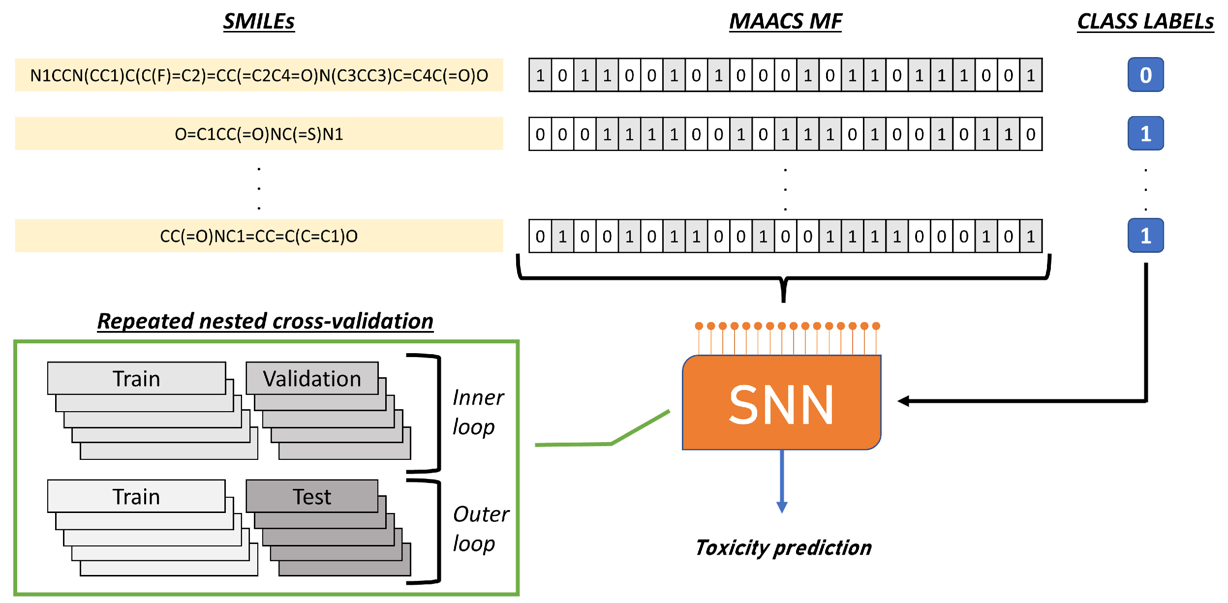
4. Materials and Methods
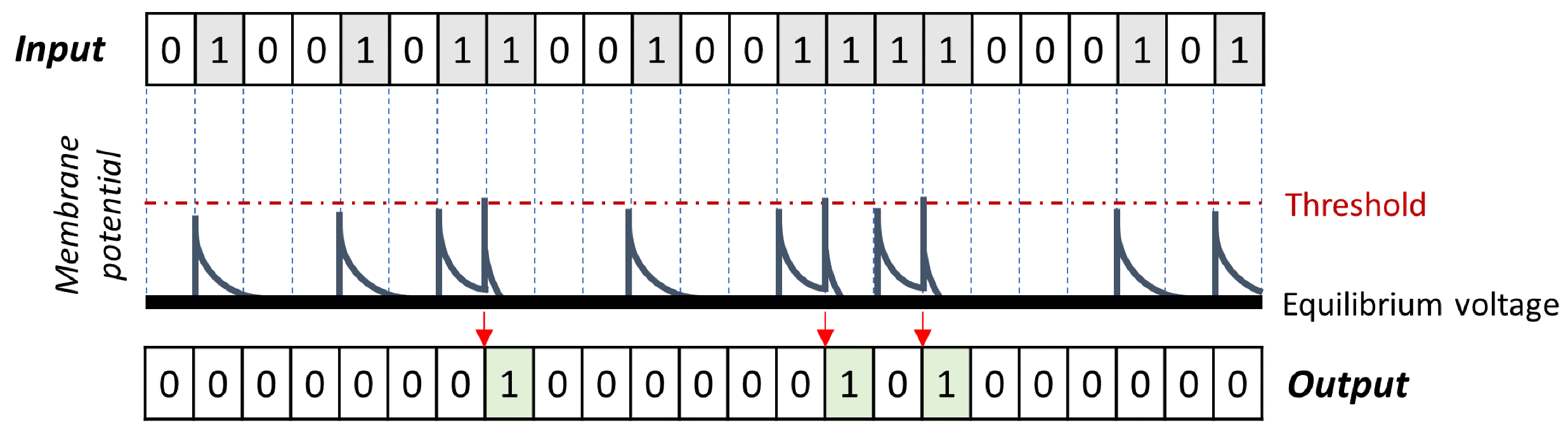
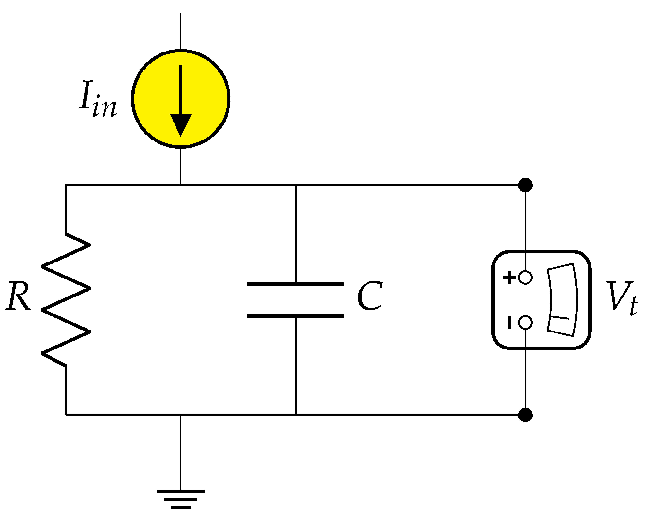
Five public-domain toxicological datasets were investigated, each evaluated in separate numerical experiments through specific SNNs. All SNNs had in common the neuronal model, the leaky integrate-and-fire (i.e., LIF) [64], and the architecture. An overview of the experimental sequence is illustrated in Figure 4.

4.1. Neuron Model

Compared to normal cells, biological neurons have peculiar features such as dendrites to capture incoming external signals, an axon to transmit pulses at a distance, and terminal parts called synapses to forward information to the dendrites of other neurons. Through the axon, information is transmitted temporarily varying the concentration gradient of transmembrane ions. This change affects the axon from the beginning to the end, creating a charged ionic flow similar to electric currents in a cable [65]. When a neuron receives inputs from the dendrites, the cell body weighs all ionic charges received, and if the total signal is enough, the cell’s polarity changes. This initial polarization influences the axon membrane gradient that is modified due to the influx of positive ions. Ions rapidly move inside the neuron through ionic channels following gradient concentrations sequentially along the neuron membrane up to the synapse. Once the process is moving toward the synapse, a short hyperpolarization called the refractory period is accompanied by restoring the equilibrium potential by accumulating outside the neuron positively charged ionic species. The complexity of these biological mechanisms is simplified using the single-compartment LIF neurons: the weighted sum of inputs (aka “integration”) triggers ionic changes across the membrane (aka “firing”) [66]. However, the integrator is “leaky” because a small amount becomes lost while integrating inputs over time. The membrane potential fluctuations resulting from the received input sequences are exemplified in Figure 5. The ones in the incoming stimuli are represented as square current pulses that disrupt the ionic equilibrium between axonal cytosol and extracellular fluid, eventually generating a spike (ones in the output sequence). Single perturbations are not enough to activate the neuron response (firing), whereas multiple stimuli overcoming the voltage threshold (red dashed line) elicit a response. After a neuronal spike, the voltage drops rapidly to a hyperpolarization state; later, the neuron is ready to respond again—single stimuli below the threshold return to equilibrium with a slower decay rate than in the case of hyperpolarization. Figure 5 does not explicitly show hyperpolarization but summarizes the different decay to equilibrium in case of firing or not. In the neurophysiological nomenclature, the neuron membrane depolarization responding to an over-threshold input stimulus is called action potential or spike, meaning the neuron is firing and usually marked with a one in a vector describing the neuron activity over time. Mathematically, this could be associated with a Heaviside step function. Periods of below-threshold stimuli are equivalent to zeros, meaning no firing occurs on the neuron membrane. The binary sequences describing neurons’ activity are formally equivalent to bit strings of molecular fingerprints; this aspect allows for a direct usage of MFs as input for SNNs, and no format conversion is needed.
A first-order low-pass filter could represent a leaky integrator, and from this assumption, the LIF equations are described mathematically in terms of electrical circuits [67]. Ions passing the neuron membrane wall experience a resistance R and are subject to a capacitance C: the resistance depicts the narrowness of the membrane’s ion channels that slow down the influx, and the capacitance is the lipidic membrane bilayer acting as an insulator (Figure 6).
Considering the time constant of the circuit is τ = R C , Equation (1) describes variations of the LIF membrane potentials as voltage shifts measured by the voltmeter in Figure 6.
τ d V t d t = V t + R I i n
The linear ordinary differential equation could be solved with the forward Euler method for practical application in the SNN. Another characteristic of neurons is the hyperpolarization following a membrane depolarization or firing. This could be achieved with a reset mechanism subtracting a fixed voltage value until reaching equilibrium or simply resetting the voltage to zero; all SNNs were assembled with the first reset option by subtraction.

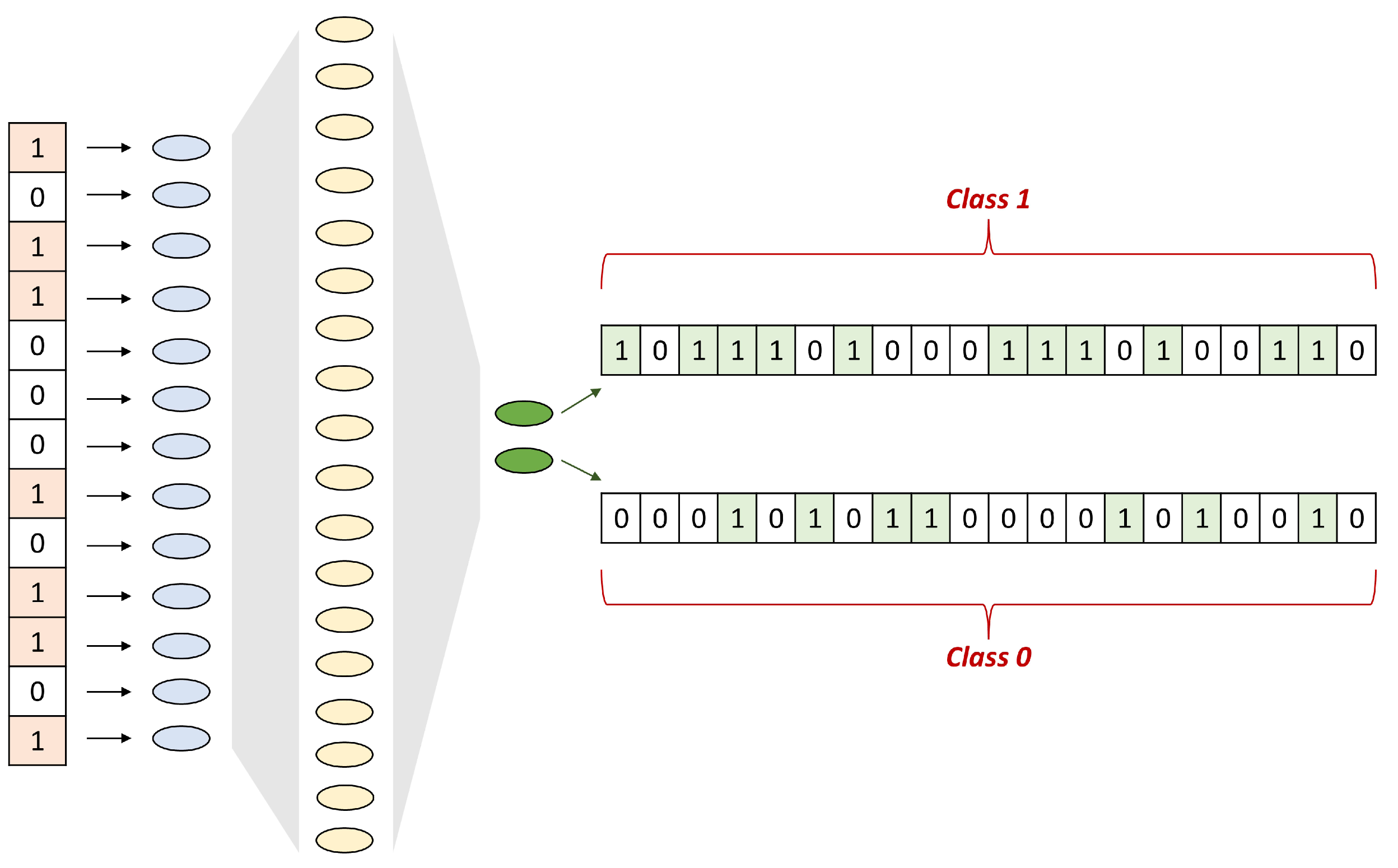
4.2. SNN Architecture

The SNNs were programmed in Python language, using Torch and derived libraries [68,69]. All networks had the same number of input neurons, equal to the number of bits in the fingerprints’ vectors, one hidden layer, and an output layer of two neurons, as shown in Figure 7. The number of hidden neurons was the subject of investigation during the hyperparameters search.
Class membership was determined by the number of spikes fired by the last two neurons, assigning it to the neuron that fired more spikes. The SNNs were fully connected with input data distributed in mini batches of 64 samples. The subdivision of the input samples in mini-batches avoided the “generalization gap” noticed with large input sample sizes [70]. The discrete nature of the binary vectors employed by SNNs poses the challenge of the lack of differentiability during backpropagation calculations through the chain rule. The solution to this problem has been proposed in [71], by applying a surrogate function that replaces the hard threshold. In other words, during backpropagation, a sigmoid activation is selected with a finite slope instead of computing the derivative of the Heaviside step function (the Dirac delta function).

4.3. Model Evaluation and Hyperparameters Tuning

Each SNN had several hyperparameters (i.e., HPs) to be tuned: in the previous literature [72,73,74], this part is usually reported as time-consuming and challenging to perform due to the non-linear relationship between LIF output and HPs. In the current investigation, nested cross-validation (i.e., CV) has been employed to separate the phase of HP optimization and model evaluation. The HP selection was achieved during the inner loop, while the outer loop evaluated model quality. Additionally, the CV has been repeated ten times to analyze model variability and generalization error extensively. Among the HPs searched, the membrane decay rate β , expressed as V t + Δ t = β × V t , and the slope of the surrogate gradient were LIF-specific. More general HPs were the number of hidden neurons, the optimizer type and its parameters, the number of epochs needed for training, and the presence or lack of gradient clipping (i.e., GC). This latter technique is mainly utilized to circumvent exploding gradient issues [75]. Another optimizer HP included was the weight decay (i.e., WD), usually adopted to regularize the network [76].
HP optimization was performed with a random search over a regularly spaced grid of values, except for the learning rate (i.e., LR) with pre-selected intervals. The search range is reported in Table 11. The optimizers implemented in the Python Torch library and surveyed were “Adam” and “Adamax” [77], “Stochastic Gradient (Descent) Optimizer” (i.e., SGO [78]), “Adaptive Gradient Algorithm” (i.e., Adagrad [79]), “Adadelta” [80], “AdamW” [81], and “RMSProp” [82].

4.4. Benchmark Datasets Employed in the Study

The compounds explored came from the following repositories, with a summary in Table 12:
  • TOXCAST [83], containing results of in vitro toxicological experiments. In particular, the outcomes for “Tox21-TR-LUC-GH3-Antagonist” were considered due to the best sample ratio;
  • Tox21 [84], predicting the toxicity on biological targets, including nuclear receptors or stress response pathways. Activities selected were “SR-ATAD5”, “NR-EL-LBD”, and “NR-AR” for the relatively low number of missing entries compared to the others inside the dataset;
  • BBBP [85] assessing drug’s blood–brain barrier penetration;
  • SIDER [86], employed for predicting drug’s side effects on the immune and nervous systems;
  • Clintox [87], containing drugs that failed or passed clinical trials for toxicity.
All of the datasets’ molecules were in the SMILES format with annotated binary labels. The number of instances was unequal in all cases, processed balancing by oversampling the minority class. If class balancing was not performed, the risk was that the classifiers may be over-exposed to the majority class during training. The last column of Table 12 reported the initial instances for the negative and positive classes and the number of examples after equalization inside parenthesis. The results of the numerical experiments were judged through balanced accuracy (i.e., BA). Although equalizing class counts could be sufficient to evaluate models fairly by accuracy, balanced accuracy further ensured unbiased appraisal.

4.5. Fingerprints Characteristics

After standardizing and normalizing the functional groups, the SMILES to fingerprint conversion was performed via the RDkit Python library [88]. Preprocessing has been performed with MolVS [89], a software tool included in RDkit. The selected MFsformat was the SMARTS-based implementation of the 166 bits long public MACCS keys.
Another preliminary aspect to verify was the similarity of the molecules inside each dataset. If the compound similarity is high, the classifier may learn representations of analogous molecular structures, affecting the model’s generalization. The heterogeneity of the molecules in each dataset was evaluated through the Jaccard–Tanimoto index and reported as mean values in Table 13. This coefficient demonstrated high reliability in quantifying molecule similarity from MF [90].
In the datasets, the probability of co-occurrences between compounds ranged from 20.8% to 33.5%, or conversely, a mean dissimilarity ranging from 79.2% to 66.5%. The Tox21 family of data and TOXCAST exhibited the most significant heterogeneity between molecules, while BBBP, Clintox, and SIDER collected closer compound types.

4.6. Meta-Analysis Criteria

Current classification results on MAACS MFs applying SNNs were compared to the previous literature for each dataset. Journal articles were selected using the Google Scholar engine, integrated with Università del Piemonte Orientale library resources. The dataset name was inserted as keyword together with “molecular fingerprint”. Pre-prints were not considered because they were not yet peer-reviewed. The article list was sorted per publication data, with the most recent on the top, and results scanned in descending order; priority was assigned to works showing outcomes on MAACS MFs for direct comparison with the current investigation. Only articles employing area under the receiver operating characteristic curve (i.e., AUC) or accuracy as evaluation metrics on the test set were considered for compatibility with current outcomes. Another precaution as inclusion criteria involved the selection of studies dividing the samples of the original datasets in random splits (consistent with Molecule Net [85]); other methods, such as scaffold splits, are usually associated with lower AUC due to increased difficulty. In a few cases, the results were presented as figures only, without providing tables to collect numerical information, and consequently, the values could not be retrieved.

5. Conclusions

This work witnessed the usage of spiking neural networks for the virtual screening of multiple databases of compounds targeting toxicity. The results were in line with top-notch predictors from the literature, opening the door to the possible usage of neuroscience-inspired artificial intelligence for quantitative structure–activity or property relationship analysis. Future works will further evaluate the applicability of spiking neural networks to other chemoinformatics domains, with the intent of employing an integrated software and hardware neuromorphic architecture.

Author Contributions

Conceptualization, M.N.; methodology, M.N.; coding, M.N.; validation, M.N.; formal analysis, M.N.; investigation, M.N.; writing—original draft preparation, M.N.; writing—review and editing, M.N. and L.R.; visualization, M.N.; supervision, L.R.; project administration, L.R.; funding acquisition, L.R. All authors have read and agreed to the published version of the manuscript.

Funding

The authors received funding from European Union’s Horizon 2020 research and innovation program under grant agreement No. 860462 project PREMUROSA.

Institutional Review Board Statement

Not applicable.

Informed Consent Statement

Not applicable.

Data Availability Statement

Benchmark datasets used in this paper were public-domain databases of molecules that can be accessed from the MoleculeNet repository [85].

Conflicts of Interest

The authors declare no conflict of interest.

Sample Availability

Not applicable.

Abbreviations

The following abbreviations are used in this manuscript:
AUCArea Under the ROC Curve
BABalanced Accuracy
CVCross-Validation
ECFPsExtended-Connectivity Fingerprints
GCGradient Clipping
HPsHyperparameters
LIFLeaky Integrate-and-Fire (neuron model)
LRLearning Rate
MFsMolecular Fingerprints
MLMachine Learning
NNNeural Network (other than SNN)
QSARQuantitative Structure–Activity Relationship
QSPRQuantitative Structure–Property Relationship
RFRandom Forest
ROCReceiver Operating Characteristic
SGOStochastic Gradient Optimizer
SMILESSimplified Molecular-Input Line-Entry System
SNNSpiking Neural Network
WDWeight Decay

Appendix A

Table A1 reports validation and test set accuracies of the nested CV rounds.
Table A1. Balanced accuracy at validation and test sets as percentages.
DatasetValidation SetTest Set
Clintox96.6 ± 0.597.8 ± 0.7
NR-AR98.8 ± 0.498.3 ± 0.5
NR-ER-LBD97.8 ± 0.498.5 ± 0.4
SR-ATAD595.0 ± 0.699.0 ± 0.2
BBBP92.7 ± 1.394.5 ± 1.1
TOXCAST89.0 ± 1.091.4 ± 0.9
NSD95.8 ± 1.197.0 ± 0.8
ISD78.5 ± 2.381.8 ± 2.0

Appendix B

Table A2 collects the AUC outcomes of [45] as described in Section 2.3.1.
Table A2. AUC from single and multiple task learning as shown in [45].
BenchmarkSingleMultiple
ISD0.670 ± 0.0380.801 ± 0.040
NSD0.820 ± 0.0830.901 ± 0.049
NR-AR0.810 ± 0.0270.851 ± 0.043
NR-ER-LBD0.898 ± 0.0400.952 ± 0.041
SR-ATAD50.844 ± 0.0330.905 ± 0.038
BBBP0.713 ± 0.006
Table A3 shows results as reported in [49] (Section 2.3.2).
Table A3. AUC on ClinTox from [49].
MethodRef.Clintox
TOP[49]0.946  ±  0.003
CheMixNet[53]0.944  ±  0.004
DeepAOT[54]0.894  ±  0.003
DeepTox[46]0.843  ±  0.003
Chemception[55]0.745  ±  0.006
SMILES2Vec[56]0.693  ±  0.004
RF 0.769  ±  0.002
SVM 0.751  ±  0.002
KNN 1 0.698 ±  0.003
1 k—nearest neighbors algorithm.
Table A4 presents AUC values from [40] (Section 2.3.2).
Table A4. AUC from the numerical experiments in [40].
BenchmarkD-MPNN 1D-MPNN (Ensemble)
BBBP0.913  ±  0.0260.925  ±  0.036
Tox210.845  ±  0.0150.861  ±  0.012
SIDER0.646  ±  0.0160.664  ±  0.021
Clintox0.894  ±  0.0270.906  ±  0.043
1 directed Message Passing NN.
Table A5 displays scores as detailed in [51] (Section 2.3.2).
Table A5. Best models AUC in [51] for Clintox and BBBP applying different MF sets.
MF TypeFeaturesBBBPClintox
SSLP-FPsC [51]0.949 ± 0.0160.963 ± 0.044
SSLP-FPsCP [51]0.953 ± 0.0090.939 ± 0.047
SSLP-FPsCPZ [51]0.946 ± 0.0150.941 ± 0.035
Auto-FPs 0.969 ± 0.010.95 ± 0.037
ECFC21024 bits0.92 ± 0.0150.821 ± 0.058
ECFC22048 bits0.919 ± 0.0210.833 ± 0.053
ECFC2512 bits0.913 ± 0.0190.831 ± 0.056
ECFC41024 bits0.914 ± 0.0240.782 ± 0.052
ECFC42048 bits0.916 ± 0.0210.784 ± 0.053
ECFC4512 bits0.908 ± 0.0250.801 ± 0.049
ECFC61024 bits0.907 ± 0.0290.77 ± 0.054
ECFC62048 bits0.911 ± 0.0260.75 ± 0.059
ECFC6512 bits0.9 ± 0.0320.77 ± 0.048

Appendix C

Table A6 reports the average number of seconds taken during the ten repetitions of nested CV ECFP analysis on BBBP and Clintox datasets. Computations were accomplished on commodity hardware (laptop computer with Intel i5 CPU and 16Gb RAM). Furthermore, the table includes the number of training epochs as a parameter directly affecting the computational time.
Table A6. Computational times for ECFP.
DatasetComputational Time (s)Training Epochs
Clintox4109.55300
BBBP1522.74100
In general, computational times could be heavily influenced by several factors (for example, the number of training epochs, the batch size, the number of parallel jobs on the computer, the use of CPU or GPU, etc.); thus, they should be evaluated considering all these aspects. Additionally, SNN architectures should be programmed on neuromorphic boards to improve computational performance because adapting SNN on traditional hardware may only highlight some advantages of this technique.

References

  1. Mitchell, J.B. Machine learning methods in chemoinformatics. Wiley Interdiscip. Rev. Comput. Mol. Sci. 2014, 4, 468–481. [Google Scholar] [CrossRef] [PubMed] [Green Version]
  2. Neves, B.J.; Braga, R.C.; Melo-Filho, C.C.; Moreira-Filho, J.T.; Muratov, E.N.; Andrade, C.H. QSAR-Based Virtual Screening: Advances and Applications in Drug Discovery. Front. Pharmacol. 2018, 9, 1275. [Google Scholar] [CrossRef] [Green Version]
  3. Cherkasov, A.; Muratov, E.N.; Fourches, D.; Varnek, A.; Baskin, I.I.; Cronin, M.; Dearden, J.; Gramatica, P.; Martin, Y.C.; Todeschini, R.; et al. QSAR modeling: Where have you been? Where are you going to? J. Med. Chem. 2014, 57, 4977–5010. [Google Scholar] [CrossRef] [Green Version]
  4. Svetnik, V.; Liaw, A.; Tong, C.; Culberson, J.C.; Sheridan, R.P.; Feuston, B.P. Random forest: A classification and regression tool for compound classification and QSAR modeling. J. Chem. Inf. Comput. Sci. 2003, 43, 1947–1958. [Google Scholar] [CrossRef]
  5. Polishchuk, P.G.; Muratov, E.N.; Artemenko, A.G.; Kolumbin, O.G.; Muratov, N.N.; Kuz’min, V.E. Application of random forest approach to QSAR prediction of aquatic toxicity. J. Chem. Inf. Model. 2009, 49, 2481–2488. [Google Scholar] [CrossRef] [PubMed]
  6. Singh, H.; Singh, S.; Singla, D.; Agarwal, S.M.; Raghava, G.P. QSAR based model for discriminating EGFR inhibitors and non-inhibitors using Random forest. Biol. Direct 2015, 10, 1–12. [Google Scholar] [CrossRef] [PubMed] [Green Version]
  7. Motamedi, F.; Pérez-Sánchez, H.; Mehridehnavi, A.; Fassihi, A.; Ghasemi, F. Accelerating big data analysis through LASSO-random forest algorithm in QSAR studies. Bioinformatics 2022, 38, 469–475. [Google Scholar] [CrossRef]
  8. Ancuceanu, R.; Dinu, M.; Neaga, I.; Laszlo, F.G.; Boda, D. Development of QSAR machine learning-based models to forecast the effect of substances on malignant melanoma cells. Oncol. Lett. 2019, 17, 4188–4196. [Google Scholar] [CrossRef]
  9. Doucet, J.P.; Barbault, F.; Xia, H.; Panaye, A.; Fan, B. Nonlinear SVM approaches to QSPR/QSAR studies and drug design. Curr. Comput. -Aided Drug Des. 2007, 3, 263–289. [Google Scholar] [CrossRef]
  10. Czermiński, R.; Yasri, A.; Hartsough, D. Use of support vector machine in pattern classification: Application to QSAR studies. Quant. Struct. -Act. Relatsh. 2001, 20, 227–240. [Google Scholar] [CrossRef]
  11. Chavan, S.; Nicholls, I.A.; Karlsson, B.C.; Rosengren, A.M.; Ballabio, D.; Consonni, V.; Todeschini, R. Towards global QSAR model building for acute toxicity: Munro database case study. Int. J. Mol. Sci. 2014, 15, 18162–18174. [Google Scholar] [CrossRef] [PubMed] [Green Version]
  12. Konovalov, D.A.; Coomans, D.; Deconinck, E.; Vander Heyden, Y. Benchmarking of QSAR models for blood–brain barrier permeation. J. Chem. Inf. Model. 2007, 47, 1648–1656. [Google Scholar] [CrossRef] [PubMed]
  13. Goh, G.B.; Hodas, N.O.; Vishnu, A. Deep learning for computational chemistry. J. Comput. Chem. 2017, 38, 1291–1307. [Google Scholar] [CrossRef] [PubMed] [Green Version]
  14. Rosenblatt, F. The perceptron: A probabilistic model for information storage and organization in the brain. Psychol. Rev. 1958, 65, 386. [Google Scholar] [CrossRef] [Green Version]
  15. Maass, W.; Bishop, C.M. Pulsed Neural Networks; MIT Press: Cambridge, MA, USA, 2001. [Google Scholar]
  16. Marković, D.; Mizrahi, A.; Querlioz, D.; Grollier, J. Physics for neuromorphic computing. Nat. Rev. Phys. 2020, 2, 499–510. [Google Scholar] [CrossRef]
  17. Roy, K.; Jaiswal, A.; Panda, P. Towards spike-based machine intelligence with neuromorphic computing. Nature 2019, 575, 607–617. [Google Scholar] [CrossRef]
  18. Gerum, R.C.; Schilling, A. Integration of leaky-integrate-and-fire neurons in standard machine learning architectures to generate hybrid networks: A surrogate gradient approach. Neural Comput. 2021, 33, 2827–2852. [Google Scholar] [CrossRef] [PubMed]
  19. Mauri, A.; Consonni, V.; Pavan, M.; Todeschini, R. Dragon software: An easy approach to molecular descriptor calculations. Match 2006, 56, 237–248. [Google Scholar]
  20. Moriwaki, H.; Tian, Y.S.; Kawashita, N.; Takagi, T. Mordred: A molecular descriptor calculator. J. Cheminformatics 2018, 10, 1–14. [Google Scholar] [CrossRef] [Green Version]
  21. Karpov, P.; Godin, G.; Tetko, I.V. Transformer-CNN: Swiss knife for QSAR modeling and interpretation. J. Cheminformatics 2020, 12, 1–12. [Google Scholar] [CrossRef] [Green Version]
  22. Hu, S.; Chen, P.; Gu, P.; Wang, B. A Deep Learning-Based Chemical System for QSAR Prediction. IEEE J. Biomed. Health Inform. 2020, 24, 3020–3028. [Google Scholar] [CrossRef] [PubMed]
  23. Atz, K.; Grisoni, F.; Schneider, G. Geometric deep learning on molecular representations. Nat. Mach. Intell. 2021, 3, 1023–1032. [Google Scholar] [CrossRef]
  24. Jin, W.; Barzilay, R.; Jaakkola, T. Junction tree variational autoencoder for molecular graph generation. In Proceedings of the International Conference on Machine Learning, PMLR, Stockholm, Sweden, 10–15 July 2018; pp. 2323–2332. [Google Scholar]
  25. Xu, K.; Hu, W.; Leskovec, J.; Jegelka, S. How powerful are graph neural networks? arXiv 2018, arXiv:1810.00826. [Google Scholar]
  26. Fung, V.; Zhang, J.; Juarez, E.; Sumpter, B.G. Benchmarking graph neural networks for materials chemistry. Npj Comput. Mater. 2021, 7, 1–8. [Google Scholar] [CrossRef]
  27. Chen, D.; Lin, Y.; Li, W.; Li, P.; Zhou, J.; Sun, X. Measuring and relieving the over-smoothing problem for graph neural networks from the topological view. In Proceedings of the AAAI Conference on Artificial Intelligence, New York, NY, USA, 7–12 February 2020; AAAI Press: Palo Alto, CA, USA, 2020; Volume 34, pp. 3438–3445. [Google Scholar]
  28. Oono, K.; Suzuki, T. Graph neural networks exponentially lose expressive power for node classification. arXiv 2019, arXiv:1905.10947. [Google Scholar]
  29. Ying, C.; Cai, T.; Luo, S.; Zheng, S.; Ke, G.; He, D.; Shen, Y.; Liu, T.Y. Do transformers really perform badly for graph representation? Adv. Neural Inf. Process. Syst. 2021, 34, 28877–28888. [Google Scholar]
  30. Wu, Z.; Zhu, M.; Kang, Y.; Leung, E.L.H.; Lei, T.; Shen, C.; Jiang, D.; Wang, Z.; Cao, D.; Hou, T. Do we need different machine learning algorithms for QSAR modeling? A comprehensive assessment of 16 machine learning algorithms on 14 QSAR data sets. Brief. Bioinform. 2021, 22, bbaa321. [Google Scholar] [CrossRef]
  31. Triolascarya, K.; Septiawan, R.R.; Kurniawan, I. QSAR Study of Larvicidal Phytocompounds as Anti-Aedes Aegypti by using GA-SVM Method. J. RESTI (Rekayasa Sist. Dan Teknol. Inf.) 2022, 6, 632–638. [Google Scholar] [CrossRef]
  32. Rahmani, N.; Abbasi-Radmoghaddam, Z.; Riahi, S.; Mohammadi-Khanaposhtanai, M. Predictive QSAR models for the anti-cancer activity of topoisomerase IIα catalytic inhibitors against breast cancer cell line HCT15: GA-MLR and LS-SVM modeling. Struct. Chem. 2020, 31, 2129–2145. [Google Scholar] [CrossRef]
  33. Wigh, D.S.; Goodman, J.M.; Lapkin, A.A. A review of molecular representation in the age of machine learning. Wiley Interdiscip. Rev. Comput. Mol. Sci. 2022, 12, e1603. [Google Scholar] [CrossRef]
  34. Durant, J.L.; Leland, B.A.; Henry, D.R.; Nourse, J.G. Reoptimization of MDL keys for use in drug discovery. J. Chem. Inf. Comput. Sci. 2002, 42, 1273–1280. [Google Scholar] [CrossRef] [Green Version]
  35. Daylight Toolkit. SMARTS-A Language for Describing Molecular Patterns; Daylight Chemical Information Systems Inc.: Aliso Viejo, CA, USA, 2007. [Google Scholar]
  36. Rogers, D.; Hahn, M. Extended-connectivity fingerprints. J. Chem. Inf. Model. 2010, 50, 742–754. [Google Scholar] [CrossRef] [PubMed]
  37. Ghosh-Dastidar, S.; Adeli, H. Spiking neural networks. Int. J. Neural Syst. 2009, 19, 295–308. [Google Scholar] [CrossRef] [Green Version]
  38. Carlson, K.D.; Nageswaran, J.M.; Dutt, N.; Krichmar, J.L. An efficient automated parameter tuning framework for spiking neural networks. Front. Neurosci. 2014, 8, 10. [Google Scholar] [CrossRef]
  39. Hassabis, D.; Kumaran, D.; Summerfield, C.; Botvinick, M. Neuroscience-inspired artificial intelligence. Neuron 2017, 95, 245–258. [Google Scholar] [CrossRef] [PubMed] [Green Version]
  40. Yang, K.; Swanson, K.; Jin, W.; Coley, C.; Eiden, P.; Gao, H.; Guzman-Perez, A.; Hopper, T.; Kelley, B.; Mathea, M.; et al. Analyzing learned molecular representations for property prediction. J. Chem. Inf. Model. 2019, 59, 3370–3388. [Google Scholar] [CrossRef] [Green Version]
  41. Yang, Q.; Liu, Y.; Cheng, J.; Li, Y.; Liu, S.; Duan, Y.; Zhang, L.; Luo, S. An Ensemble Structure and Physiochemical (SPOC) Descriptor for Machine-Learning Prediction of Chemical Reaction and Molecular Properties. ChemPhysChem 2022, 23, e202200255. [Google Scholar] [CrossRef] [PubMed]
  42. Zhang, J.; Mucs, D.; Norinder, U.; Svensson, F. LightGBM: An effective and scalable algorithm for prediction of chemical toxicity–application to the Tox21 and mutagenicity data sets. J. Chem. Inf. Model. 2019, 59, 4150–4158. [Google Scholar] [CrossRef]
  43. Jiang, J.; Wang, R.; Wei, G.W. GGL-Tox: Geometric graph learning for toxicity prediction. J. Chem. Inf. Model. 2021, 61, 1691–1700. [Google Scholar] [CrossRef]
  44. Banerjee, P.; Siramshetty, V.B.; Drwal, M.N.; Preissner, R. Computational methods for prediction of in vitro effects of new chemical structures. J. Cheminformatics 2016, 8, 1–11. [Google Scholar] [CrossRef] [PubMed] [Green Version]
  45. Jeon, W.; Kim, D. FP2VEC: A new molecular featurizer for learning molecular properties. Bioinformatics 2019, 35, 4979–4985. [Google Scholar] [CrossRef] [PubMed]
  46. Mayr, A.; Klambauer, G.; Unterthiner, T.; Hochreiter, S. DeepTox: Toxicity prediction using deep learning. Front. Environ. Sci. 2016, 3, 80. [Google Scholar] [CrossRef] [Green Version]
  47. Drwal, M.N.; Siramshetty, V.B.; Banerjee, P.; Goede, A.; Preissner, R.; Dunkel, M. Molecular similarity-based predictions of the Tox21 screening outcome. Front. Environ. Sci. 2015, 3, 54. [Google Scholar] [CrossRef] [Green Version]
  48. Idakwo, G.; Thangapandian, S.; Luttrell, J.; Li, Y.; Wang, N.; Zhou, Z.; Hong, H.; Yang, B.; Zhang, C.; Gong, P. Structure–activity relationship-based chemical classification of highly imbalanced Tox21 datasets. J. Cheminformatics 2020, 12, 1–19. [Google Scholar] [CrossRef] [PubMed]
  49. Peng, Y.; Zhang, Z.; Jiang, Q.; Guan, J.; Zhou, S. TOP: A deep mixture representation learning method for boosting molecular toxicity prediction. Methods 2020, 179, 55–64. [Google Scholar] [CrossRef] [PubMed]
  50. Dai, H.; Dai, B.; Song, L. Discriminative embeddings of latent variable models for structured data. In Proceedings of the International Conference on Machine Learning, PMLR, New York, NY, USA, 19–24 June 2016; pp. 2702–2711. [Google Scholar]
  51. Chen, D.; Zheng, J.; Wei, G.W.; Pan, F. Extracting Predictive Representations from Hundreds of Millions of Molecules. J. Phys. Chem. Lett. 2021, 12, 10793–10801. [Google Scholar] [CrossRef]
  52. Lim, S.; Lee, Y.O. Predicting chemical properties using self-attention multi-task learning based on SMILES representation. In Proceedings of the IEEE 2020 25th International Conference on Pattern Recognition (ICPR), Milan, Italy, 10–15 January 2021; pp. 3146–3153. [Google Scholar]
  53. Paul, A.; Jha, D.; Al-Bahrani, R.; Liao, W.k.; Choudhary, A.; Agrawal, A. Chemixnet: Mixed dnn architectures for predicting chemical properties using multiple molecular representations. arXiv 2018, arXiv:1811.08283. [Google Scholar]
  54. Xu, Y.; Pei, J.; Lai, L. Deep learning based regression and multiclass models for acute oral toxicity prediction with automatic chemical feature extraction. J. Chem. Inf. Model. 2017, 57, 2672–2685. [Google Scholar] [CrossRef]
  55. Goh, G.B.; Siegel, C.; Vishnu, A.; Hodas, N.O.; Baker, N. Chemception: A deep neural network with minimal chemistry knowledge matches the performance of expert-developed QSAR/QSPR models. arXiv 2017, arXiv:1706.06689. [Google Scholar]
  56. Goh, G.B.; Siegel, C.; Vishnu, A.; Hodas, N. Using rule-based labels for weak supervised learning: A ChemNet for transferable chemical property prediction. In Proceedings of the 24th ACM SIGKDD International Conference on Knowledge Discovery & Data Mining, London, UK, 19–23 August 2018; pp. 302–310. [Google Scholar]
  57. Zou, X.; Xu, S.; Chen, X.; Yan, L.; Han, Y. Breaking the von Neumann bottleneck: Architecture-level processing-in-memory technology. Sci. China Inf. Sci. 2021, 64, 1–10. [Google Scholar] [CrossRef]
  58. Young, A.R.; Dean, M.E.; Plank, J.S.; Rose, G.S. A review of spiking neuromorphic hardware communication systems. IEEE Access 2019, 7, 135606–135620. [Google Scholar] [CrossRef]
  59. Kaiser, F.; Feldbusch, F. Building a bridge between spiking and artificial neural networks. In Proceedings of the International Conference on Artificial Neural Networks, Porto, Portugal, 9–13 September 2007; Springer: Berlin/Heidelberg, Germany, 2007; pp. 380–389. [Google Scholar]
  60. Rao, V.R.; Finkbeiner, S. NMDA and AMPA receptors: Old channels, new tricks. Trends Neurosci. 2007, 30, 284–291. [Google Scholar] [CrossRef] [PubMed]
  61. Moreno-Bote, R.; Parga, N. Simple model neurons with AMPA and NMDA filters: Role of synaptic time scales. Neurocomputing 2005, 65, 441–448. [Google Scholar] [CrossRef]
  62. Rao, A.; Plank, P.; Wild, A.; Maass, W. A Long Short-Term Memory for AI Applications in Spike-based Neuromorphic Hardware. Nat. Mach. Intell. 2022, 4, 467–479. [Google Scholar] [CrossRef]
  63. Ruiz Puentes, P.; Valderrama, N.; González, C.; Daza, L.; Muñoz-Camargo, C.; Cruz, J.C.; Arbeláez, P. PharmaNet: Pharmaceutical discovery with deep recurrent neural networks. PLoS ONE 2021, 16, e0241728. [Google Scholar] [CrossRef] [PubMed]
  64. Burkitt, A.N. A review of the integrate-and-fire neuron model: I. Homogeneous synaptic input. Biol. Cybern. 2006, 95, 1–19. [Google Scholar] [CrossRef]
  65. Fukutome, H.; Tamura, H.; Sugata, K. An electric analogue of the neuron. Kybernetik 1963, 2, 28–32. [Google Scholar] [CrossRef]
  66. Dayan, P.; Abbott, L.F. Theoretical Neuroscience: Computational and Mathematical Modeling of Neural Systems; MIT Press: Cambridge, MA, USA, 2005. [Google Scholar]
  67. Brunel, N.; Van Rossum, M.C. Lapicque’s 1907 paper: From frogs to integrate-and-fire. Biol. Cybern. 2007, 97, 337–339. [Google Scholar] [CrossRef]
  68. Paszke, A.; Gross, S.; Massa, F.; Lerer, A.; Bradbury, J.; Chanan, G.; Killeen, T.; Lin, Z.; Gimelshein, N.; Antiga, L.; et al. Pytorch: An imperative style, high-performance deep learning library. Adv. Neural Inf. Process. Syst. 2019, 32. [Google Scholar] [CrossRef]
  69. Eshraghian, J.K.; Ward, M.; Neftci, E.; Wang, X.; Lenz, G.; Dwivedi, G.; Bennamoun, M.; Jeong, D.S.; Lu, W.D. Training spiking neural networks using lessons from deep learning. arXiv 2021, arXiv:2109.12894. [Google Scholar]
  70. Oyedotun, O.K.; Papadopoulos, K.; Aouada, D. A new perspective for understanding generalization gap of deep neural networks trained with large batch sizes. Appl. Intell. 2022, 1–17. [Google Scholar] [CrossRef]
  71. Neftci, E.O.; Mostafa, H.; Zenke, F. Surrogate gradient learning in spiking neural networks: Bringing the power of gradient-based optimization to spiking neural networks. IEEE Signal Process. Mag. 2019, 36, 51–63. [Google Scholar] [CrossRef]
  72. Russell, A.; Orchard, G.; Dong, Y.; Mihalaş, Ş.; Niebur, E.; Tapson, J.; Etienne-Cummings, R. Optimization methods for spiking neurons and networks. IEEE Trans. Neural Netw. 2010, 21, 1950–1962. [Google Scholar] [CrossRef] [PubMed] [Green Version]
  73. Guo, W.; Yantır, H.E.; Fouda, M.E.; Eltawil, A.M.; Salama, K.N. Toward the optimal design and FPGA implementation of spiking neural networks. IEEE Trans. Neural Netw. Learn. Syst. 2021, 33, 3988–4002. [Google Scholar] [CrossRef]
  74. Manna, D.L.; Vicente-Sola, A.; Kirkland, P.; Bihl, T.; Di Caterina, G. Simple and complex spiking neurons: Perspectives and analysis in a simple STDP scenario. Neuromorphic Comput. Eng. 2022, 2, 044009. [Google Scholar] [CrossRef]
  75. Zhang, J.; He, T.; Sra, S.; Jadbabaie, A. Why gradient clipping accelerates training: A theoretical justification for adaptivity. arXiv 2019, arXiv:1905.11881. [Google Scholar]
  76. Krogh, A.; Hertz, J. A simple weight decay can improve generalization. Adv. Neural Inf. Process. Syst. 1991, 4, 950–957. [Google Scholar]
  77. Kingma, D.P.; Ba, J. Adam: A method for stochastic optimization. arXiv 2014, arXiv:1412.6980. [Google Scholar]
  78. Sutskever, I.; Martens, J.; Dahl, G.; Hinton, G. On the importance of initialization and momentum in deep learning. In Proceedings of the International Conference on Machine Learning, PMLR, Atlanta, GA, USA, 16–21 June 2013; pp. 1139–1147. [Google Scholar]
  79. Duchi, J.; Hazan, E.; Singer, Y. Adaptive subgradient methods for online learning and stochastic optimization. J. Mach. Learn. Res. 2011, 12, 2121–2159. [Google Scholar]
  80. Zeiler, M.D. Adadelta: An adaptive learning rate method. arXiv 2012, arXiv:1212.5701. [Google Scholar]
  81. Loshchilov, I.; Hutter, F. Decoupled weight decay regularization. arXiv 2017, arXiv:1711.05101. [Google Scholar]
  82. Hinton, G.; Srivastava, N.; Swersky, K. Neural networks for machine learning lecture 6a overview of mini-batch gradient descent. Cited 2012, 14, 2. [Google Scholar]
  83. Judson, R.S.; Houck, K.A.; Kavlock, R.J.; Knudsen, T.B.; Martin, M.T.; Mortensen, H.M.; Reif, D.M.; Rotroff, D.M.; Shah, I.; Richard, A.M.; et al. In vitro screening of environmental chemicals for targeted testing prioritization: The ToxCast project. Environ. Health Perspect. 2010, 118, 485–492. [Google Scholar] [CrossRef] [PubMed] [Green Version]
  84. Richard, A.M.; Huang, R.; Waidyanatha, S.; Shinn, P.; Collins, B.J.; Thillainadarajah, I.; Grulke, C.M.; Williams, A.J.; Lougee, R.R.; Judson, R.S.; et al. The Tox21 10K compound library: Collaborative chemistry advancing toxicology. Chem. Res. Toxicol. 2020, 34, 189–216. [Google Scholar] [CrossRef] [PubMed]
  85. Wu, Z.; Ramsundar, B.; Feinberg, E.N.; Gomes, J.; Geniesse, C.; Pappu, A.S.; Leswing, K.; Pande, V. MoleculeNet: A benchmark for molecular machine learning. Chem. Sci. 2018, 9, 513–530. [Google Scholar] [CrossRef] [Green Version]
  86. Kuhn, M.; Letunic, I.; Jensen, L.J.; Bork, P. The SIDER database of drugs and side effects. Nucleic Acids Res. 2016, 44, D1075–D1079. [Google Scholar] [CrossRef]
  87. Gayvert, K.M.; Madhukar, N.S.; Elemento, O. A data-driven approach to predicting successes and failures of clinical trials. Cell Chem. Biol. 2016, 23, 1294–1301. [Google Scholar] [CrossRef]
  88. Landrum, G. RDKit: A software suite for cheminformatics, computational chemistry, and predictive modeling. Greg Landrum 2013, 8. [Google Scholar] [CrossRef]
  89. Swain, M. MolVS: Molecule Validation and Standardization. Available online: https://molvs.readthedocs.io/en/latest/ (accessed on 15 August 2022).
  90. Bajusz, D.; Rácz, A.; Héberger, K. Why is Tanimoto index an appropriate choice for fingerprint-based similarity calculations? J. Cheminformatics 2015, 7, 1–13. [Google Scholar] [CrossRef]
Figure 1. Visual summary of meta-analysis on Tox21. Standard deviation was included if reported in the original papers. AUC values from [40,41,42,43,44,45,47,48].
Molecules 28 01342 g001
Figure 2. Classification of side effects of chemicals from SIDER dataset in the present and other works. AUC included from [45,52].
Molecules 28 01342 g002
Figure 3. Outcomes for BBBP and Clintox compared to the previous literature. AUC values as reported in [40,41,46,49,51,53,54,55,56].
Molecules 28 01342 g003
Figure 4. Overview of the procedure during the numerical experiments. The input bit strings were created from SMILES, and a binary label accompanied each instance. The binary sequences were input directly to the SNN, which was evaluated by nested cross-validation with an inner loop for model selection and an outer loop for evaluating the quality of the outcomes.
Molecules 28 01342 g004
Figure 5. Membrane potential in LIF neurons is modeled receiving a binary train as input and producing a binary output in response: only when membrane potential is over-threshold do LIF neurons fire a spike marked by ones in the output sequence.
Molecules 28 01342 g005
Figure 6. LIF circuit equivalent. A parallel resistor and capacitor represent the neuron, a configuration that could easily describe membrane behavior and, at the same time, is effortlessly implementable on silicon chips.
Molecules 28 01342 g006
Figure 7. Exemplification of the common SNN architectures. All SNNs employed were shallow with one hidden layer. The fingerprints’ bits were passed to the input layer, whereas the last layer firing counts determined the predicted class.
Molecules 28 01342 g007
Table 1. Results on Clintox.
Hidden Neur. β Grad. SlopeOpt.LRWDGCMean BAStd BA
10000.875Adam0.00010True97.8450.661
10000.6550Adam1 × 10−50True97.6630.605
10000.625Adam0.00010True97.6690.317
10000.9550Adam1 × 10−50True97.5300.774
10000.825Adam0.00010False97.3390.556
Table 2. Results on Tox21 NR-AR.
Hidden Neur. β Grad. SlopeOpt.LRWDGCMean BAStd BA
10000.9550Adagrad0.010False98.8400.368
10000.9550AdamW0.00010False98.8290.232
10000.9550Adamax0.0020False98.8230.369
15000.9550Adam5 × 10−50False98.8100.215
8000.9550Adam5 × 10−50False98.7780.241
Table 3. Results on Tox21 NR-ER-LBD.
Hidden Neur. β Grad. SlopeOpt.LRWDGCMean BAStd BA
10000.9550Adamax0.0020False98.4910.399
12000.8575Adam1 × 10−50False98.4570.270
10000.9550Adagrad0.010False98.4560.268
10000.9550Adam0.00010.001False98.3540.373
10000.9550SGO0.0010False98.2830.362
Table 4. Results on Tox21 SR-ATAD5.
Hidden Neur. β Grad. SlopeOpt.LRWDGCMean BAStd BA
12000.8575Adam1 × 10−50False99.0550.232
10000.9550Adam0.00010.001False98.8370.257
10000.9550Adagrad0.010False98.8180.182
15000.9550SGO0.0050.001False98.7980.221
10000.9550Adam0.00010False98.7950.251
Table 5. Results on TOXCAST TR-LUC-GH3-Ant.
Hidden Neur. β Grad. SlopeOpt.LRWDGCMean BAStd BA
10000.9550Adamax0.0020False91.3790.819
10000.9550Adamax0.0020.0001False91.3580.417
12000.9550Adamax0.0020False91.1900.877
10000.9550Adagrad0.010.001False91.1660.391
12000.9550Adagrad0.010False91.1380.699
Table 6. Results on BBBP.
Hidden Neur. β Grad. SlopeOpt.LRWDGCMean BAStd BA
10000.9550Adamax0.0020False94.4811.068
10000.9550SGO0.0050False94.2301.342
10000.9550RMSProp0.0010False93.8831.434
10000.825Adam0.00010False93.8380.696
10000.9550Adam0.00010False93.6511.005
Table 7. Results on SIDER ISD.
Hidden Neur. β Grad. SlopeOpt.LRWDGCMean BAStd BA
10000.9550Adagrad0.010False81.7502.027
15000.9550SGO0.0050.001False81.3761.998
10000.9550SGO0.0010False81.2543.243
20000.9550Adagrad0.010False80.9811.905
10000.825Adagrad0.010False80.9371.721
Table 8. Results on SIDER NSD.
Hidden Neur. β Grad. SlopeOpt.LRWDGCMean BAStd BA
10000.9550SGO0.0010.001False96.9780.740
10000.9550Adadelta1.00False96.5201.197
10000.9550Adagrad0.010False96.5151.211
10000.9550AdamW1 × 10−50True96.4500.840
10000.9550Adamax0.0020False96.3740.697
Table 9. Summary of SNNs’ HPs for top-ranked models.
DatasetHidden Neur. β Grad. SlopeMean BAStd BAMean AUCStd AUC
BBBP10000.955094.4811.0680.9460.008
Clintox10000.87597.8450.6610.9740.01
ISD10000.955081.7502.0270.7950.008
NR-AR10000.955098.8400.3680.9880.002
NR-ER-LBD10000.955098.4910.3990.9860.003
NSD10000.955096.9770.7400.970.008
SR-ATAD512000.857599.0550.2320.9910.002
TOXCAST10000.955091.3790.8190.9120.007
Table 10. BA of SNNs with MFs of different length as input patterns.
MF TypeBBBPClintox
ECFP93.451 ± 0.68497.772 ± 0.522
MAACS94.481 ± 1.06897.845 ± 0.661
Table 11. Parameter grid range during HP tuning. The goal was to identify the HP configuration driving the learning process to reach the best performance on each benchmark dataset.
HyperparameterLower LimitUpper LimitLevels
Hidden neurons50020005
β 0.60.956
Grad. slope25753
LR1 × 10−50.515
WD0.0010.054
Table 12. Datasets information.
DatasetActivity StudiedAcronymInstances
ClintoxToxicity in clinical trialsClintox1366 (1366)–112 (1366)
Tox21Androgen receptor nipple retentionNR-AR6956 (6956)–309 (6956)
Tox21HepatotoxicityNR-ER-LBD6605 (6605)–350 (6605)
Tox21DNA damageSR-ATAD56808 (6808)–264 (6808)
TOXCASTThyroid homeostasis disruptionTR-LUC-GH3-Ant 16170 (6170)–1761 (6170)
BBBPBlood–brain barrier permeabilityBBBP479 (1560)–1560 (1560)
SIDERImmune system disorders (iatrogenic toxicity)ISD403 (1024)–1024 (1024)
SIDERNervous system disorders (iatrogenic toxicity)NSD123 (1304)–1304 (1304)
1 Murine tissue assays.
Table 13. Mean Tanimoto indices of each dataset.
DatasetTanimoto Index
Clintox0.315
NR-AR0.21
NR-ER-LBD0.209
SR-ATAD50.208
TR-LUC-GH3-Ant0.211
BBBP0.335
ISD0.308
NSD0.308
Disclaimer/Publisher’s Note: The statements, opinions and data contained in all publications are solely those of the individual author(s) and contributor(s) and not of MDPI and/or the editor(s). MDPI and/or the editor(s) disclaim responsibility for any injury to people or property resulting from any ideas, methods, instructions or products referred to in the content.

