Article

Monitoring the Spring Flood in Lena Delta with Hydrodynamic Modeling Based on SAR Satellite Products

1
German Aerospace Center (DLR), German Remote Sensing Data Center (DFD), 82234 Wessling, Germany
2
Hydrology and River Basin Management, Technical University of Munich (TUM), 80333 Munich, Germany
3
Sachverständigenbüro für Luftbildauswertung und Umweltfragen (SLU), 81243 Munich, Germany
4
Alfred-Wegener-Institut (AWI), 14401 Potsdam, Germany
*
Author to whom correspondence should be addressed.
Remote Sens. 2021, 13(22), 4695; https://doi.org/10.3390/rs13224695
Submission received: 26 October 2021 / Revised: 16 November 2021 / Accepted: 16 November 2021 / Published: 20 November 2021
(This article belongs to the Special Issue Wetland Monitoring Using Remote Sensing)

Abstract

:
Due to the remote location and the extreme climate, monitoring stations in Arctic rivers such as Lena in Siberia have been decreasing through time. Every year, after a long harsh winter, the accumulated snow on the Lena watershed melts, leading to the major annual spring flood event causing heavy transport of sediments, organic carbon, and trace metals, both into as well as within the delta. This study aims to analyze the hydrodynamic processes of the spring flood taking place every year in the Lena Delta. Thus, a combination of remote sensing techniques and hydrodynamic modeling methodologies is used to overcome limitations caused by missing ground-truth data. As a test site for this feasibility study, the outlet of the Lena River to its delta was selected. Lena Delta is an extensive wetland spanning from northeast Siberia into the Arctic Ocean. Spaceborne Synthetic Aperture Radar (SAR) data of the TerraSAR-X/TanDEM-X satellite mission served as input for the hydrodynamic modeling software HEC-RAS. The model resulted in inundation areas, flood depths, and flow velocities. The model accuracy assessed by comparing the multi-temporal modeled inundation areas with the satellite-derived inundation areas ranged between 65 and 95%, with kappa coefficients ranging between 0.78 and 0.97, showing moderate to almost perfect levels of agreement between the two inundation boundaries. Modeling results of high flow discharges show a better agreement with the satellite-derived inundation areas compared to that of lower flow discharges. Overall, the remote-sensing-based hydrodynamic modeling succeeded in indicating the increase and decrease in the inundation areas, flood depths, and flow velocities during the annual flood events.

1. Introduction

The Lena is one of the four largest Arctic watersheds, the others being Mackenzie, Ob, and Yenisei [1]. These Arctic watersheds drain into the Arctic Ocean, influencing the sea ice cover and the ocean conveyor belt [2], which significantly affects the Earth’s radiation budget. Among its impacts is the 7% rise of the recorded average annual freshwater discharge from the six largest Eurasian rivers to the Arctic Ocean in the last century [3]. This direct impact makes Arctic surface water crucial for environment- and climate-related studies. However, despite the importance, field data measurements on these remote areas are challenging and costly.
Over the past few decades, the number of hydrological monitoring stations in Arctic regions decreased dramatically [4,5]. Due to this, various studies related to the Arctic hydrological cycle were hindered and this resulted in large error margins [6]. The limited number of openly available datasets was not sufficient to derive important information, especially compared to the vast extent and the complexity of the prospective area. Remote sensing technologies can be utilized to address this issue.
Data acquired by remote sensing platforms can be used as alternatives to gauged data where field measurements are difficult to perform. A large variety of remote sensing platforms are available in various ranges of temporal and spatial coverage. Previous studies have utilized satellite imageries to measure the river hydrological and hydrodynamic components such as inundation areas, flow velocities, soil moisture, land cover, and surface roughness. Smith and Pavelsky [7] derived rating curves of a braided river from inundation area and the reach length using MODIS imageries; the time lag between the upstream and downstream stations was used to approximate the average propagation speed. Kääb et al. [8], on the other hand, tracked river ice debris with ASTER imageries over a time period of about one minute to measure the ice and water velocity field. Baghdadi et al. [9] used the radar satellite TerraSAR-X imageries and the optical satellite Kompsat-2 images to retrieve soil moistures. Bachofer et al. [10] performed topsoil classification using the imageries of Worldview-2, ASTER, TerraSAR-X, and ENVISAT ASAR with the DEM derived from SRTM-X. Aubert et al. [11] derived soil parameters—moisture content, surface roughness, soil composition, and slaking crust—from TerraSAR-X imageries. Sadeh et al. [12] derived Manning’s roughness coefficient from (COSMO)-SkyMed SAR imageries.
This study aims to integrate information derived from datasets of the twin radar satellite TerraSAR-X and TanDEM-X (hereafter TSX/TDX) into a hydrodynamic model to monitor the spring flood in a subset of the Lena Delta, an extensive wetland spanning from northeast Siberia into the Arctic Ocean. The hydrodynamic model was set up by using the Hydrologic Engineering Center’s River Analysis System (HEC-RAS) developed by the US Army Corps of Engineers. It is an open-source software package that is widely used in many studies and research that incorporate geospatial datasets [13,14,15]. Previously, TSX/TDX datasets have been used for studies of the wetland environment [16]. TSX datasets have been previously used to detect the major seasonal land surface changes [17] and observe the cliff-top erosion on the Lena Delta riverbanks [18] in the Lena Delta. These studies show that the X-band signal can provide detailed insights into the permafrost environmental conditions, albeit the retrieval can be heavily affected by vegetation layers. The integration of remote sensing and flood modeling has been emerging in river sciences [19]. Heimhuber [13], Krötzinger [14], and Hong Quang et al. [15] have performed hydrodynamic modeling with HEC-RAS using input data derived from the twin radar satellite TSX/TDX datasets. They derived inundation boundaries from TSX/TDX Stripmap products and used the global Digital Elevation Model (DEM) from TanDEM-X (hereafter TDX-DEM) to derive the surface terrain elevation (i.e., topography). As the radar signal does not penetrate water, TDX-DEM does not show the elevations of the riverbed terrain (i.e., bathymetry), which is an important input in hydrodynamic modeling. Heimhuber [13] and Krötzinger [14] incorporate supplemental information on river bathymetry from field acquisition and LiDAR.
In this study, we assessed the feasibility of monitoring and observing the hydrodynamic processes of the spring flood event in the Lena Delta with mainly remotely sensed data and limited field data. In contrast to the aforementioned previous studies, this study site represents a complex geomorphology of a braided river system and bathymetry data are not available, hence they were to be estimated iteratively according to the model results. The HEC-RAS one-dimensional (1D) modeling module was selected due to the lack of in situ data. Two- and three-dimensional models of such a vast area would require more detailed inputs and show computational drawbacks, which is especially of importance in large study areas. Although the TSX/TDX-DEM is of high spatial resolution and is able to provide detailed floodplain terrain, the river bathymetry was completely unknown; hence it had to be estimated. The estimated bathymetry lacks the complexity and heterogeneity of the real riverbed. Therefore, we chose to use a simpler 1D approach. In 1D modeling, the river channels and floodplains are considered to be a continuous series of cross-sectional profiles and water flows only on the x-axis. HEC-RAS 1D modeling module was found to perform well even when compared to more sophisticated modeling approaches [20,21]. Moreover, considering the large size of the Lena Delta, the 1D module enables modeling of the whole extent. A study by Caruso et al. [22] has successfully performed HEC-RAS 1D modeling on a complex braided river system comparable to the characteristics of the Lena Delta. The expected results of the hydrodynamic modeling are multi-temporal inundation areas, flood depths, and flow velocities of the annual spring flood events occurring between 2013 and 2019. During this time span, the most severe flood occurred in 2014 and the discharge of the flood events kept declining towards 2019.

2. Materials and Methods
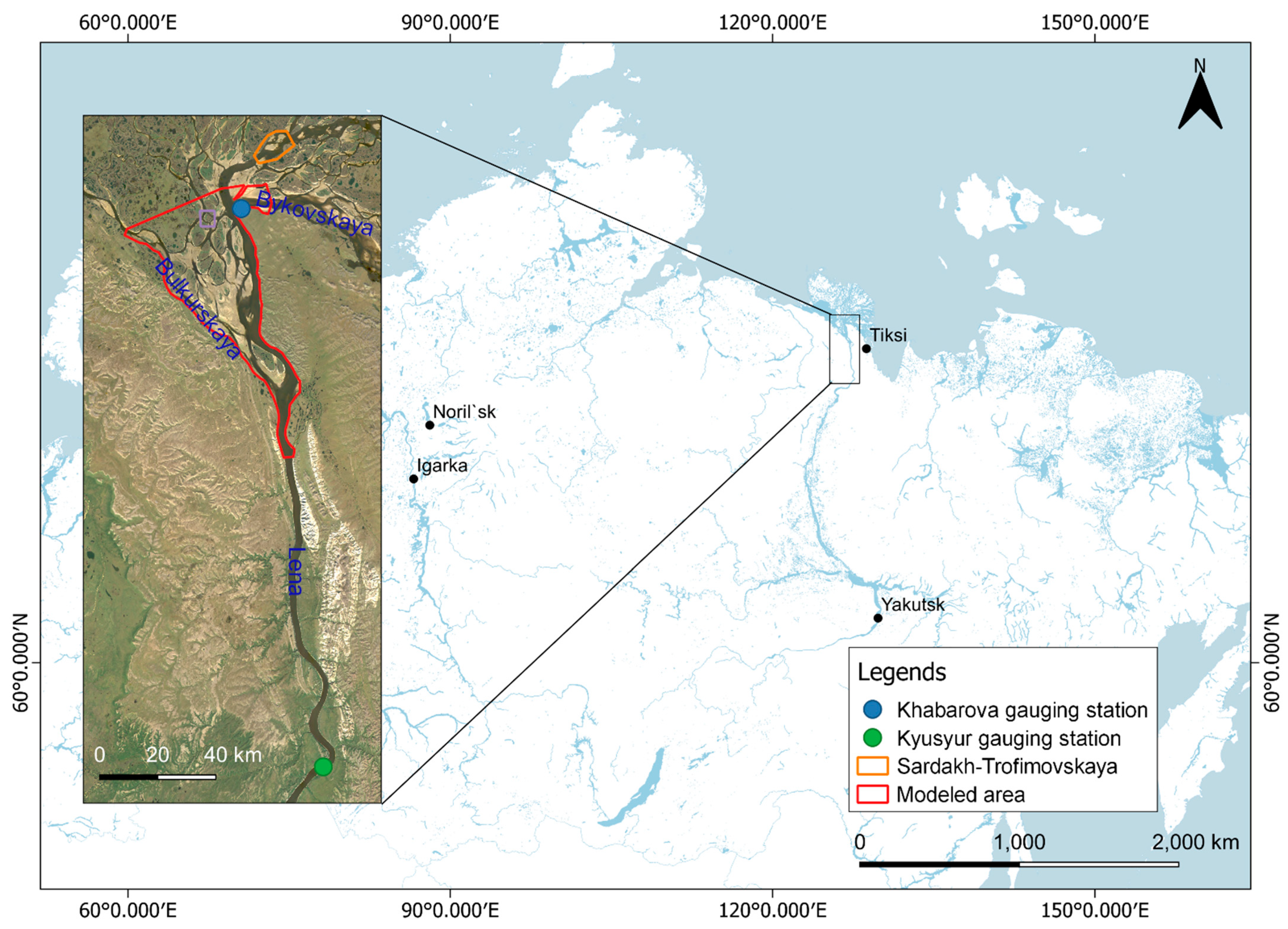
2.1. Study Site

The Lena River is the 10th longest natural river in the world [5] located in eastern Siberia. The river basin is 2.4 × 10⁶ km2 in size and 4500 km [23] in length. This river basin releases an annual average water discharge of more than 500 km3 [24]. The Lena River generally remains frozen from early December to late April and then thaws into a vast wetland on the river delta. The ice thawing coincides with the annual peak flow in June [24]. The spring flood that occurs from May to June [25,26] affects the floodplain ecology due to the heavy transport of trace metals, organic carbon, and sediment that occurs [4]. The permafrost ecology and the water volume released to the sea are important as they are strong indicators of climate change in the Arctic.
Our aim is to monitor the spring flood in Lena Delta; however, performing hydrodynamic modeling for the entire delta (32,000 km2 [23] in size) requires extremely heavy computational work. Therefore, in this study, as a test site, we focus on a subset of Lena Delta where the river branches off to four major tributaries as seen in the inset map in Figure 1. The study site consists of a braided river system—a common river system on wetlands—flowing northwards that includes the Lena Reach, the Bulkurskaya Reach, and the Bykovskaya Reach, enclaved by cliffs on its east and west side. The area in red lines in Figure 1 indicates the selected area for the hydrodynamic modeling, which is 1561 km2 in size and 93 km in length. The green dot shows the gauging station in Kyusyur that recorded the water discharge 124.65 km upstream of the modeled area. Another gauging station located on Bykovskaya Reach (marked with the blue dot) recorded the surface water level. The area in orange lines downstream of the simulated area is the location where a river morphology study was conducted—between Sardakh and Trofimovskaya Islands—by Fedorova et al. [27], which was used as the base of our bathymetry estimation. The Lena Delta riverbank sediments mainly consist of yedoma—fine-grained materials rich in organics and ice—which are common in Siberia [18]. The surrounding land surfaces consist of tundra and non-vegetated plains (sand and rock) [28,29]. The spring flood inundates the low floodplains and the shallow gullies that are usually dry in the other months.

2.2. Data

2.2.1. Remotely Sensed Datasets

The global coverage and the high resolution of the radar twin satellites TSX/TDX make it possible for users to retrieve relatively dense information for the surface of remote areas such as the Lena River Delta. In this study, data from the optical satellite missions RapidEye (hereafter RE) by Planet and Landsat 8 (hereafter LS8) by USGS were utilized as supplementary datasets where the information from the TSX/TDX in our library was not sufficient. Table 1 shows the specifications of the remotely sensed datasets used as well as the derived hydrodynamic parameters. Radar satellites TSX/TDX transmit pulses and receive the backscatter, whereas optical satellites RE and LS8 capture surface reflectance. These four satellites differ in area coverage (swath width), spatial resolution, and temporal resolution (revisit cycle) as well.
TSX/TDX are twin satellites operated by the German Aerospace Center (DLR), for which commercial exploitation rights are exclusively granted to Airbus Defense and Space [31]. The satellites are equipped with Synthetic Aperture Radar (SAR) sensors operating in the X band (9.65 GHz). Although this platform has a revisit cycle of 11 days, the study area Lena Delta is covered by numerous TSX/TDX Stripmap tiles of various orbits, making it possible to have coverage almost on a daily basis with the gap of 2–5 days. From a collection of the available TSX/TDX Stripmap acquisitions between 2013 and 2019, 38 Stripmap products were used for multi-temporal analysis and the model input. These products consist of varying polarizations (dual-co HHVV or dual-cross HHHV), incidence angles, and pass directions (ascending or descending); therefore, different scenes covered the study site on different acquisition days. On specific days, multiple scenes were needed to cover the study sites. The TDX-DEM product over the study area was generated from three TSX/TDX acquisitions in 2011 when the surface water level was at the lowest; on 29 January, 28 September, and 31 October. The TDX-DEM was oversampled from its original spacing of 12.5 m to 5 m spacing of the TSX/TDX Stripmap imagery to enable a one-to-one comparison. This step comprised an edge preserving filtering as described in Huber et al. [32]. TDX global DEM has relative and absolute vertical accuracies of 2 m and 10 m, respectively. This DEM product represents the cover on top of the earth’s surface including water bodies, vegetation, and manmade objects and is therefore a digital surface model [33].
RE is a constellation of five optical satellites with a spatial resolution of 5 m [34]. Available RE Ortho—Level 3A images were provided by Alfred Wegener Institute. The image acquired on 9 July 2014 was selected due to the least cloud cover percentage among the available images. LS8 is an optical satellite that utilizes Operational Land Imager (OLI) and Thermal Infrared Sensor (TIRS) with a spatial resolution of 30 m [35]. LS8 7-band Level-2 Surface Reflectance datasets were available for free by request through the USGS Earth Explorer [36]. An LS8 image acquired on 9 July 2014 was selected for its low land cloud cover percentage. These RE and LS8 imageries were used to derive information on the area that was not covered by the available TSX/TDX and RE imageries.

2.2.2. Field Datasets
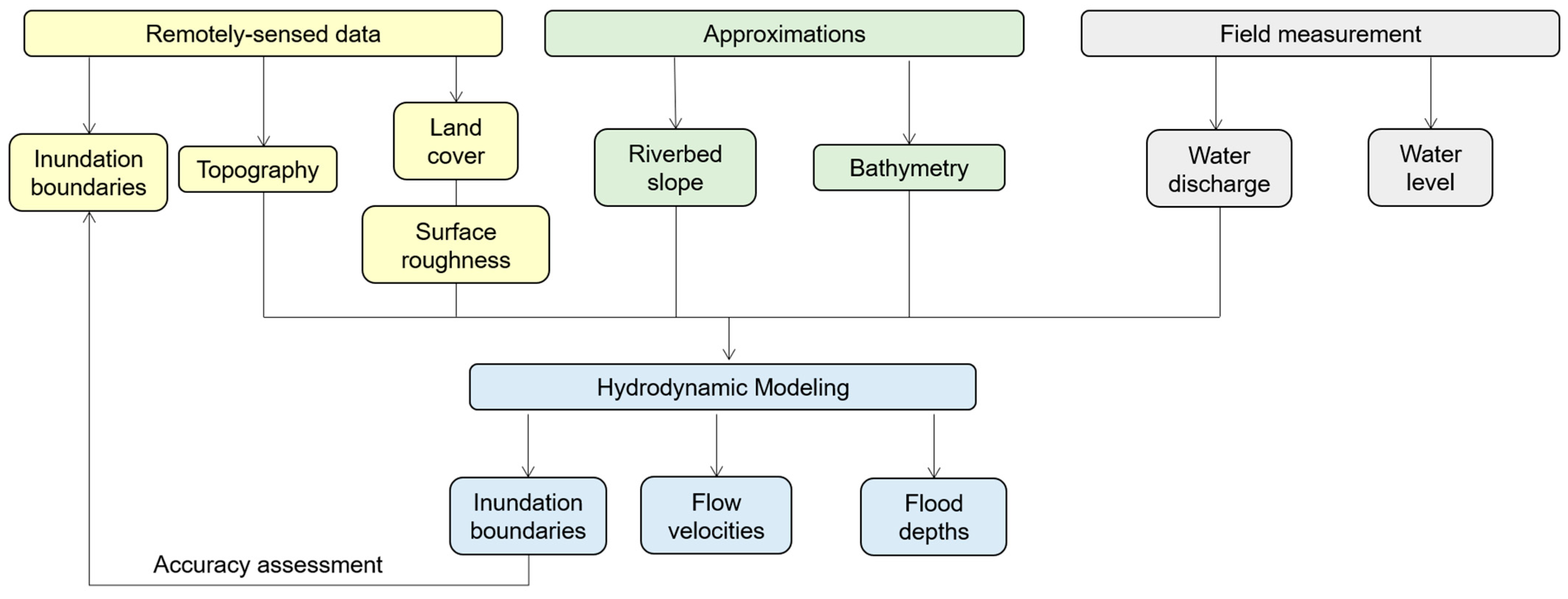
The field datasets consist of in situ upstream river discharge and surface water level elevation datasets. Average daily water discharge datasets were acquired through the Arctic Great Rivers Observatory (ArcticGRO)’s website [37], recorded at a gauging station in Kyusyur (70.68° N, 127.39° E) (location in Figure 1). The water level datasets were available through the Russian Ministry of Natural Resources and Environment’s website [26], recorded at a gauging station in Khabarova, located on Bykovskaya Reach (Figure 1 However, the exact coordinate information of Khabarova station was not given. Khabarova and Kyusyur stations are located roughly 200 km away from each other. Therefore, the flood peaked at different times at these two stations, with an average discrepancy of two days. Figure 2a,b show the time-series plot of the in situ upstream river discharge and surface water level elevation.

2.3. Methodology

This subsection explains the steps of remote sensing and the hydrodynamic modeling methodologies (Figure 3). The remote sensing methodology consists of image pre-processing, inundation boundary mapping, land cover classification, bathymetry estimation, and geospatial data conversion to HEC-RAS model input format. The hydrodynamic modeling methodology comprises the flow data (river discharge) preparation, simulation setup, model stabilization, and model accuracy assessments. The flood events were modeled in three different stages each year: (1) before the flood; (2) the flood peak; and (3) after the flood. Therefore, in total, we have 21 model cases spanning from 2013 to 2019.
Important hydrodynamic input data such as river bathymetry, river flow direction, and weather information were not openly available for this site. Additionally, input data needed to calibrate the model results such as the flow velocity were also not available. Therefore, these information gaps were filled with assumptions. In order to estimate the bathymetry, the river channels were assumed to be trapezoidal and the depths were determined through an iterative process with rough initial values taken from a study on the Lena Delta sedimentation by Fedorova et al. [27]. Through this study, we found out that the river depths between these two islands range between −10 and −30 m and are very dynamic due to the heavy sediment transport. Weather effects on the watershed—which might strongly influence the flow in such a large watershed—as well as floating ice and frozen channels were neglected. The river flow was assumed to be one-dimensional (1D) from the south to the north with the selected 1D modeling module.
One image of each of the TSX/TDX, RE, and LS8 datasets was used to map land cover of the study site, through which the Manning’s surface roughness coefficient values of the floodplain were derived. Additionally, the inundation areas were mapped using the multi-temporal TSX/TDX imagery which has high revisit frequency as well as high resolution. The derived Manning’s surface roughness coefficients, the in situ river discharge recorded at Kyusyur station, and the estimated bathymetry were fed into the model which was built with the open-source hydrodynamic modeling software, HEC-RAS version 5.0.7 by the US Army Corps of Engineers. The model accuracies were assessed by comparing the modeled inundation areas with the remotely sensed inundation areas.

2.3.1. Remote Sensing Methods

Image Pre-Processing

The remote sensing part of the methodology started with SAR satellite imagery pre-processing to correct and calibrate the TSX/TDX datasets prior to the analysis. We processed 38 TSX/TDX single look complex datasets for visual multi-temporal analysis and flood mapping. These files were converted into geocoded and radiometrically calibrated Kennaugh element multiband raster layers using the DLR Multi-SAR processor. Kennaugh elements describe the polarimetric information of the physical scattering mechanism of SAR images, consisting of 10 elements [38]. This process comprises radiometric calibration, polarimetric decomposition, multi-looking, Range-Doppler ortho-rectification, reducing multiplicative noise, and Multi-scale Multilooking and Schmittlet image enhancement. Dual-co-polarized HHVV imageries were converted into raster files with the total intensity of HH and VV (K0), ratio between the HH and VV phase, i.e., double bounce and surface scattering (K3), ratio between HH and VV intensity (K4), and the phase shift between the HH and VV phase centers (K7) bands [38]. Dual-cross-polarized HHHV imageries were converted into raster files with the total intensity of HH and VV (K0) and the difference of the HH and HV intensities [38].
Furthermore, mean-shift image segmentation was applied to the TSX/TDX Stripmap products (from the previous step), RE Ortho—Level 3, and LS8 L2 Surface Reflectance imageries. Amongst other segmentation methods, mean-shift was selected because it considers the neighboring cells, which works better in reducing heterogeneity in mixed pixel values of high spatial imageries. Mean-shift image segmentation was performed with spatial detail of five and spectral detail of 20, resulting in images with high spectral detail and low spatial detail. The segmented images then were to be utilized for inundation boundary generation, land cover classification, and bathymetry estimation.

Inundation Boundary Mapping

The TDX-DEM and 38 pre-processed and segmented multi-temporal TSX/TDX Stripmap products were used as the input for the estimation of inundation areas of the 21 model cases. Previous studies [19,39,40] recommend HH polarization for flooded area discrimination due to the lower sensitivity to wind-induced surface roughness as VV. Nevertheless, water and land areas were not always easily numerically distinguishable due to the existence of floating ice covers, still noticeable wind effects at steep incidence angles, and limited discrimination of calm water and flat, muddy river banks soaked with water at low incidence angles, as seen in Figure 4a–c. Therefore, instead of using classification methods, the inundation boundaries were generated by image-fitting and visual interpretation. The DEM was flooded starting from the elevation of −6 m to 6 m with the increment of 25 cm. After a collection of inundation boundaries with varying thresholds was produced, these inundation boundaries were overlaid onto the TSX/TDX images. The inundation boundary which visually fitted the water body in a TSX/TDX image was selected as the inundation boundary of the corresponding day. This process resulted in 21 inundation boundary raster files—of three cases each year spanning from 2013 to 2019 which were used to validate the HEC-RAS hydrodynamic model accuracy; thus, they are referred to as the reference inundation boundaries from here on.

Land Cover Classification and Manning’s Surface Roughness Coefficient Estimation

The Manning’s surface roughness coefficient values were estimated based on the type of the surface cover [10]. Land cover classification was performed on the segmented TSX/TDX and RE, and imageries were classified to derive the surface roughness coefficient. The TSX/TDX and RE datasets were stacked together into an image composite due to the same spatial resolution, while LS8 composite was classified separately. The selected classification methods were unsupervised machine learning method Iso-clustering [39] and supervised machine learning method Random Forest [40]. Iso-clustering was performed to separate the classes as well as to create the training input for the Random Forest classifier. The resulting classes then were labeled based on a previous study by Schneider et al. [28] and field information from Heim [29]. Random Forest feature importance (Variable Importance Measure, VIM) was analyzed to narrow the input to the relevant bands; bands with low feature importance were omitted. In order to assess the classifier accuracy, generated stratified sample points were split into training sample points (70%) and test sample points (30%). Manning’s surface roughness coefficient values based on Chow [41] were assigned to each land cover class. From our analysis, we derived six land cover classes as discussed in the Results and Discussions sections (Table 2).

Bathymetry Estimation

Due to the missing bathymetry data, the approach to gain the whole riverbed elevation for model input was based on approximations. Well-known methods for bathymetry estimation such as empirical expressions [42,43,44] or regression-based satellite-derived bathymetry (SDB) methods [45,46] require in situ bathymetric points for calibration and validation. Moreover, SDB approaches using optical satellite imageries require information on the benthic reflectance which is only retrievable through clear water [46]. We performed Stumpf log-linear regression SDB method [45] using RE imagery in our study site. This attempt resulted in noisy surface elevation due to the high turbidity on the river reaches, as the suspended sediments in the water hindered the light attenuation to the riverbed. The channel bathymetry was therefore approximated and interpolated under the assumption that these channels have a trapezoidal shape. The slopes of these trapezoidal channels were manually drawn along the main river channels as contour lines that are gradually changing from the river banks onto the deepest part of each channel and interpolated with the Inverse Distance Weighing (IDW) method. The smaller and shallower channels were not estimated with this approach because during lower river discharge, these channels were dried, hence the riverbed profiles were obtained through the TDX DEM acquisitions. These procedures were performed five times, each with different maximum depth: −30 m, −25 m, −20 m, −15 m, and −10 m (based on the range of channel depth in a study by Fedorova et al. [27] on a cross-section between the Sardakh and Trofimovskaya Islands, location shown in Figure 1) for the whole cross-sectional profile of the river, resulting in five bathymetry maps. The selected bathymetry map was selected through an iterative process. Each of these estimated bathymetry sets was fed as input of preliminary HEC-RAS hydrodynamic models. The bathymetry map that resulted in best-fitting modeled inundation areas was selected as the final bathymetry input.

The Geospatial Dataset Conversion

RiverGIS QGIS extension was utilized to extract the geospatial data values from inundation boundary mapping, land cover classification, and bathymetry information and convert them into HEC-RAS geometry input. Four geometry lines were digitized along the channels: stream centerlines, cross-sectional cutlines, bank lines, and flow paths. Then, the geospatial data values were extracted onto these lines, each with different IDs. At the end of the process, the collected database was converted into SDF, a geometry file format that is recognizable by HEC-RAS.

2.3.2. Hydrodynamic Modeling
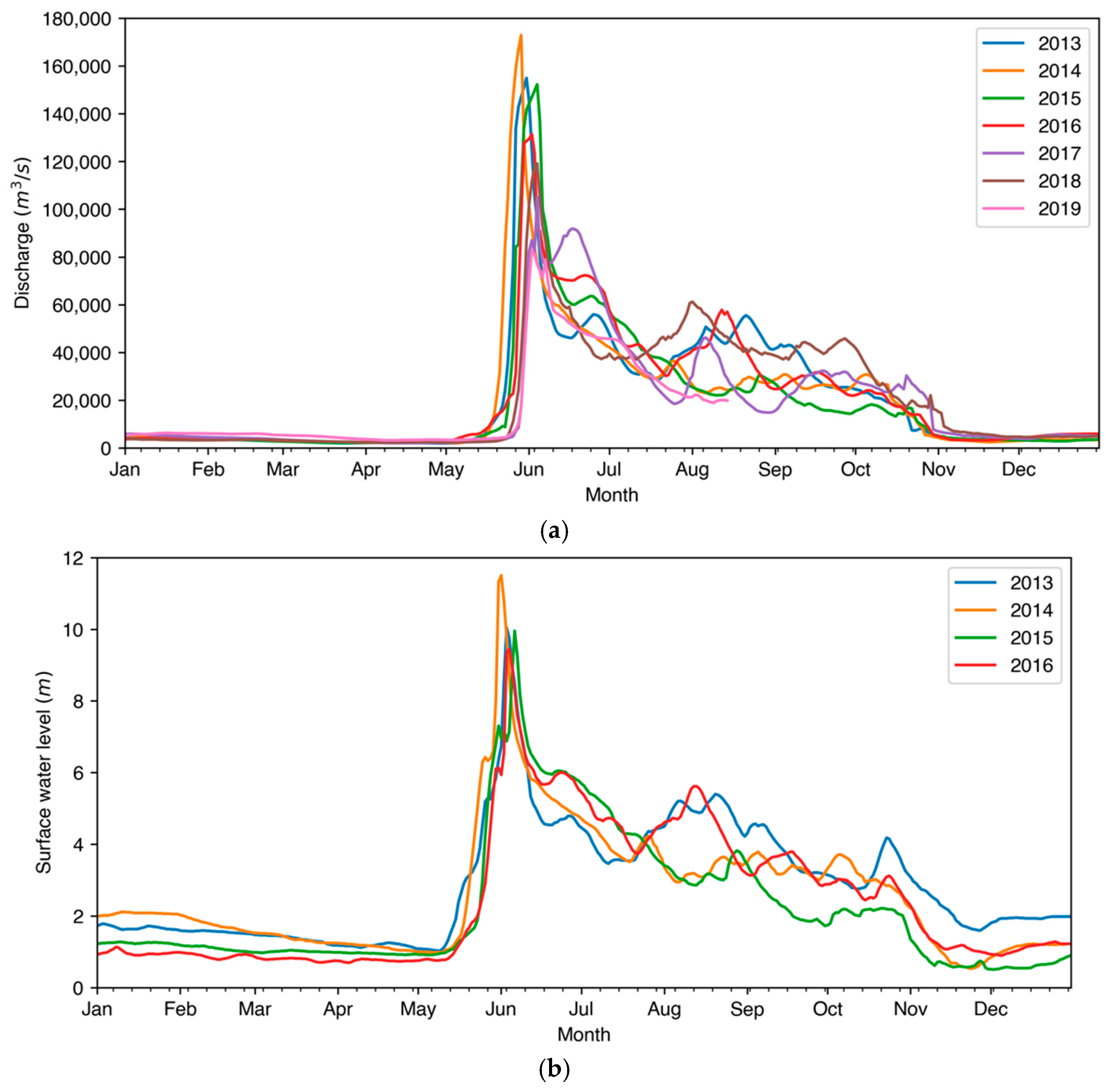
This study implemented the HEC-RAS one-dimensional (1D) unsteady flow routing for the hydrodynamic computations. During low discharge, some parts of the Lena Delta reaches were dried. Dry channels would cause an unstable model; therefore, the braided river system with the same flow direction was regarded as a single streamline, following the concept of a study by Caruso et al. [22]. Three main reaches—the upstream Lena, downstream Lena, and Bykovskaya—were digitized, connected with a junction.
The 1D unsteady flow (dynamic wave) in open channels was originally mathematically expressed by Barre de Saint-Venant in 1871 [47]. The mathematical expressions were thus acknowledged as the Saint-Venant equation [48]. This equation is based on the two conservation equations, i.e., mass and momentum [48]. The conservation of mass is based on a control volume and is expressed as follows:
( A V ) x + A t q = 0
The conservation of momentum is expressed as follows:
Q t + Q V x + g A ( h x + S f ) = 0
where A is the cross-sectional flow area, V is the flow velocity, q is the lateral in-/outflow per unit length, Q ( x , t ) is the flow at the center of the control volume, Δ x is the distance between cross sections, g is the gravity force term that is proportional to the bed slope ( S 0 ), h is the surface water level, and S f is the friction slope term. The friction slope S f is calculated as follows:
S f = n 2 V 2 R h 4 / 3
where n is the Manning’s roughness value and R h is the hydraulic radius of the channel. The conservation of momentum consists of three different terms: local acceleration, convective acceleration, and pressure force. Q t , the local acceleration term, is the change in momentum due to the change in flow velocity over time. Q V x , the convective acceleration term, is the change in momentum due to the change in flow velocity along the channel. h x , the pressure force term, is proportional to the change of depth along the channel.
The flow velocity and the surface water level are two dependent parameters varying in space and time, which are computed with simplified assumptions as the analytical solution for these equations is not available [22]. With these simplifications, the flow is regarded as one-dimensional, the water level across a single cross-sectional area is horizontal, and the channel slope is small (<0.1). Finite difference with the implicit solution scheme is used by HEC-RAS to approximate the solutions. The flow equations are expressed in finite difference form for all computational reaches with the length of Δx between the first and the last cross-section for the unknown Q and V (or h) for each time step (Δt). The information from the entire reach can influence the solution at any point.

Flow Data

The in situ discharge data served as the boundary condition in the form of a hydrograph. The input hydrograph was a constant discharge value for five days in an hourly interval to fill the channel and stabilize the model. The annual spring flood events were modeled in three different stages: before the flood (low upstream discharge), the flood peak (the highest upstream discharge), and after the flood (upstream discharge values between the low and the highest ones). The discharge values before the flood range from 2720 m3/s to 5366 m3/s between 4 and 19 May each year. The discharge values of the flood peak range from 83,000 m3/s to 173,000 m3/s between 31 May and 6 June each year. The discharge values after the flood range from 46,200 m3/s to 70,900 m3/s when the flood recedes between 11 June and 29 June each year. These three stages were selected as they specifically represent three different conditions: (1) when the thawing process had not fully started and the upstream discharge was low; (2) when the water thawed completely and filled the basin; and (3) after the flood receded and the channels were still filled with water. The complete flow data—including the upstream and two downstream discharges—are presented in the Supplementary MaterialsTable S1.

Model Setup

The model setup consisted of geometry import, adjusting the geometry, and flow data input. The imported geometry was adjusted to HEC-RAS computing capacity. The flow data were fed as an input for both steady and unsteady simulations. The steady simulation was performed prior to the unsteady simulation to obtain the parameters needed to stabilize the unsteady model. A model is stable when the temporal and spatial changes of the parameters are gradual. In this study, the main parameters tuned to stabilize the model are the cross-sectional line spacing and computational time-step. Cross-sectional line spacing ( Δ x ) was adjusted according to the Samuel equation [49], by implementing the ratio of the channel bankfull depth (D) and the overall slope (S), as follows:
Δ x 0.15   D S

Model Accuracy Assessments

The 21 reference inundation boundary maps previously derived from the TSX/TDX Stripmap products were used to validate the model results. Accuracy scores of each model were quantified with the percentage ratio of the modeled flooded pixels and the reference flooded pixels (i.e., the true positive (hit) rate from the error matrices). Kappa coefficients were also calculated to estimate the level of agreement between the modeled and reference flooded pixels of all study cases.

3. Results

3.1. Pre-Modeling Results

This section describes and displays the results of bathymetry estimation and land cover mapping and Manning’s surface roughness coefficient estimation. These two results were fed into HEC-RAS as model inputs. The estimated bathymetry was merged into the TDX DEM and served as the geometry input. The Manning’s surface roughness coefficients are required for the computation based on the Saint-Venant equation.

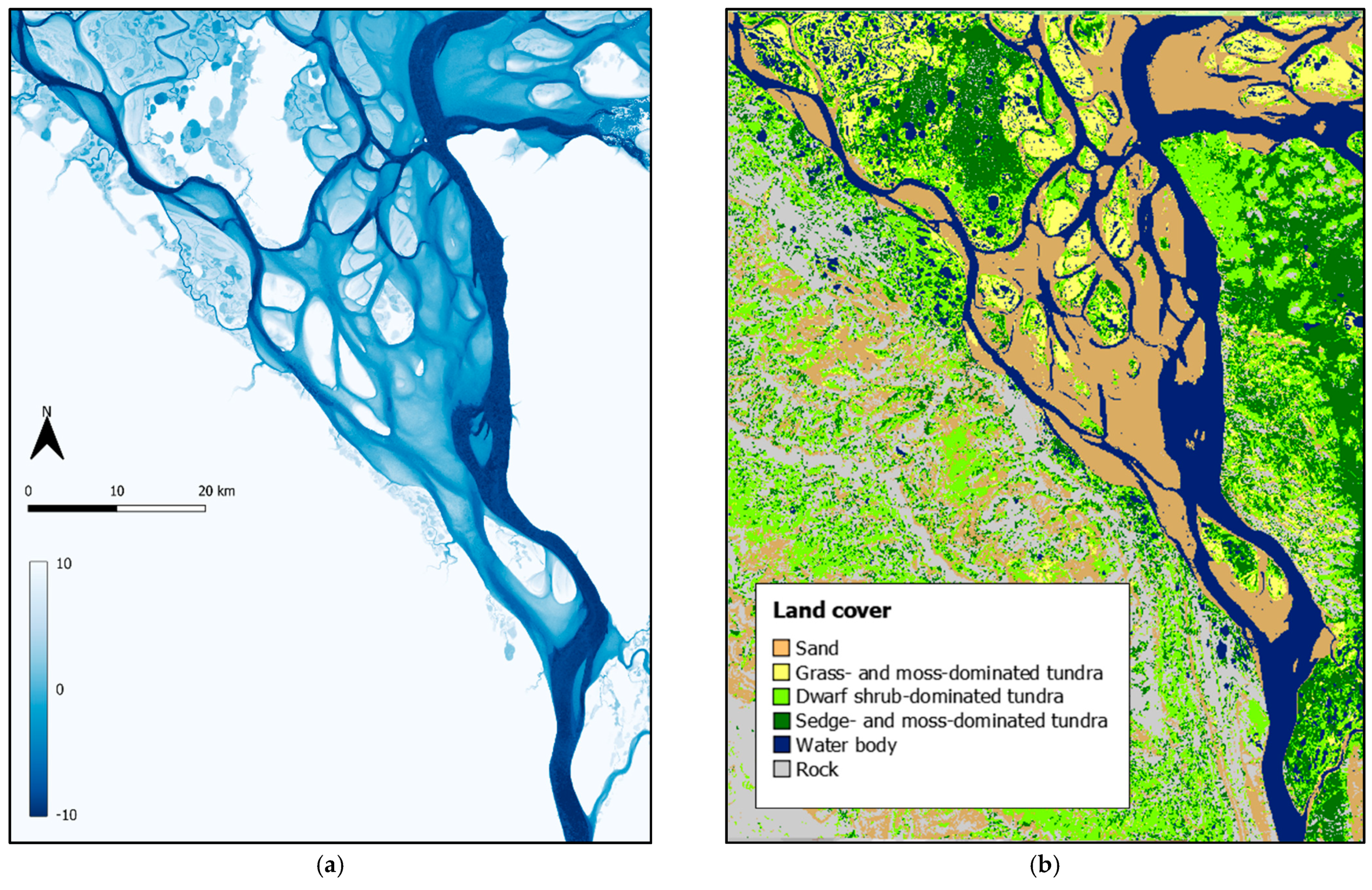
3.1.1. Estimated Bathymetry

The hydrodynamic model with the input of the bathymetry map with the −10 m maximum depth resulted in inundation areas that fitted closest to the reference inundation boundaries. Therefore, we selected this map for the final model input. The modeled inundation boundary maps from the preliminary hydrodynamic models using the bathymetry maps with the maximum depths of −30 m, −25 m, −20 m, and −15 m were underestimated, which means that only the Lena Reach was filled with water whereas the other tributaries, gullies, and low floodplains were completely dry even during the peak of the flood, showing that the depths were overestimated. The selected bathymetry map is illustrated in Figure 5a.

3.1.2. Land Cover Map and Manning’s Surface Roughness Coefficient

Figure 5b shows the land cover map of six land cover classes; sand, grass- and moss-dominated tundra, dwarf-shrub-dominated tundra, sedge- and moss-dominated tundra, water body, and rock [28,29]. The overall accuracy score of the land cover classification with the TSX/TDX-RE image composite was 94%. The overall accuracy of the land cover classification using the LS8 imagery was 75%. Compared to the LS8 land cover map, the TSX/TDX-RE land cover map provided far better details especially on the floodplains and river banks. Therefore, when these two maps were merged together to form the final land cover map, on the area where the TSX/TDX-RE map intersected with the LS8 map, the TSX/TDX-RE pixels were selected. In order to merge these two maps, the LS8 land cover map was resampled from 30 m to 5 m resolution in order to match the TSX/TDX-RE’s spatial resolution. Manning’s roughness coefficient (n) values were assigned to each land cover class. These coefficients were the averaged coefficient values according to Chow [41], presented in Table 2. The Lena Delta riverbed was mostly made of sand [27]. Therefore, the water body class was considered to be sandy riverbed.

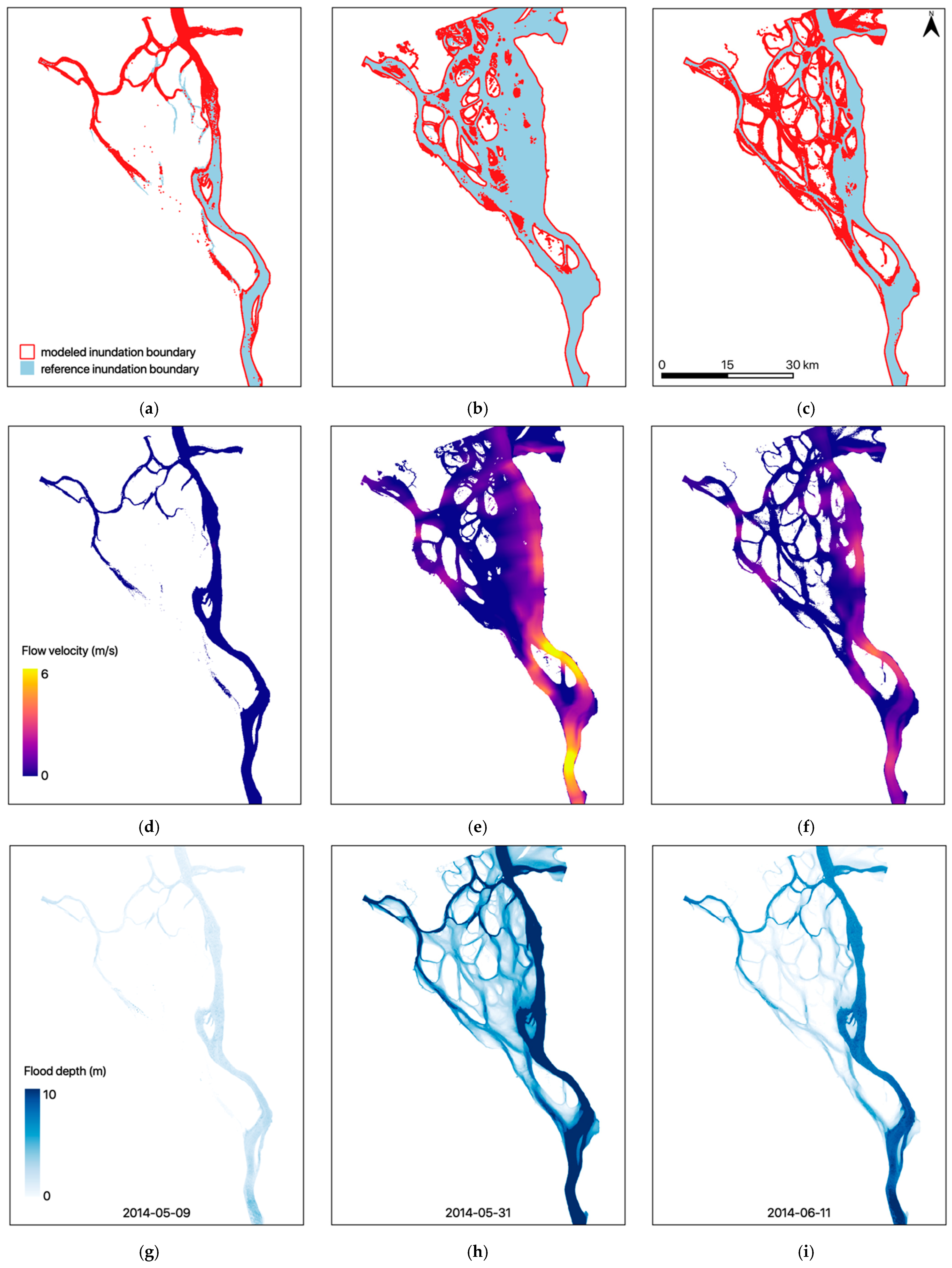
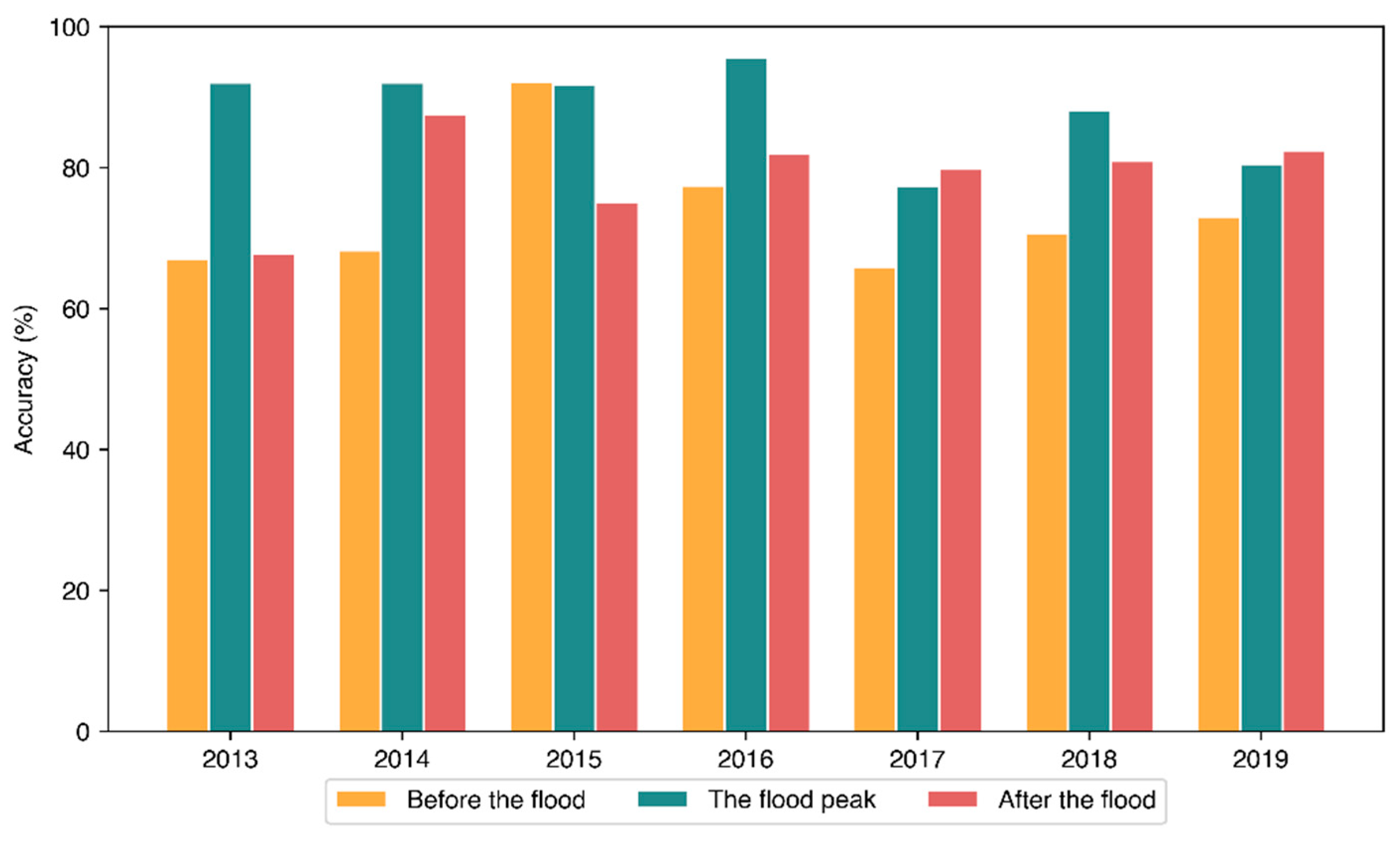
3.2. Model Accuracy Assessments with Inundation Boundaries

Figure 6a–c show only the inundation areas of the 2014 flood event, which was the most severe flood in our observation period of 2013–2019. All modeled and reference inundation areas are illustrated in the Supplementary Material—Figures S1 and S2. Figures S3 and S4 show the floodplain extents that were inundated during the flood peak. Figures S3 and S4 show smaller inundation areas in 2017 and 2019 compared to the other years, which happens to be in accordance with the decline of the discharge values through the years. The inundation areas before the flood range from 300.71 to 333.86 km2. The inundation areas during the flood peak range from 866.80 to 1118.71 km2. The inundation areas after the flood range from 604.94 to 785.40 km2. Table S2 shows the inundation areas of all the modeled events.
The accuracy scores range from 65.97 to 95.65%. The bar plot of the model accuracy scores and the model upstream discharges (Figure 7) shows that the accuracy scores of the peak flood are higher than those of the two other stages. The model accuracy scores range between 65 and 92% before the flood, 77 and 95% during the flood peak, and 67 and 87% after the flood. The same trends can be seen in the kappa coefficients (in Table S5). The kappa coefficients range from 0.78 to 0.97; between 0.78 and 0.95 before the flood (moderate to almost perfect level of agreement), 0.86 and 0.97 during the flood peak (strong to almost perfect level of agreement), and 0.76 and 0.91 after the flood (moderate to almost perfect agreement).

3.3. Modeling Results

3.3.1. Flood Depth

Figure 6g–i show the simulated water depth before the flood (early May), during the flood peak (late May), and after the flood (mid-June) in 2014. The flood depth on the floodplains of all flood events is illustrated in Figures S5 and S6. The ranges of flood depth on the floodplains are presented in Table S3. During the peak of the 2014 flood event, the floodplains with relatively lower elevations were submerged up to 5.12 m.

3.3.2. Flow Velocity

The HEC-RAS 1D unsteady flow module computes the flow velocity on the main, left overbank, and right overbank channel separately in one dimension: flow is only modeled from the upstream to the downstream in one direction. Figure 6d–f showcase the modeled flow velocity on the 2014 flood event before the flood, during the peak of the flood, and after the flood, respectively. Through the illustration, we observe that the flow velocity rose at some parts of the channel during the flood peak and then decreased again when the flood was receding. In the 2014 flood event, the modeled flow velocity prior to the flood event was up to 1.34 m/s; then the velocity built up to 6.13 m/s on some parts of the channel during the peak of the flood. The modeled flow velocities of all the flood events are depicted in Figures S7 and S8 and the ranges of the values are presented in Table S4.

4. Discussions

By combining the TDX-DEM and estimated bathymetry as the HEC-RAS geometry input together with the approximated Manning’s n values, the inundation boundaries were closely modeled, with better accuracies during the flood event when the upstream discharge values were higher. With our bathymetry estimation approach, the heterogeneities of the riverbed were neglected due to the unavailability of the channel data for calibration. Through Figure 6a–c, Figures S1 and S2, we can observe that the inundation areas were underpredicted as some of the small reaches were not filled by water.
Previous studies have reported flow velocities estimated around our study sites. Pavelsky and Smith [7], whose study site was located far south from our study site, reported the average propagation speed of 1.01 m/s, which was close to the data recorded at a station in Tabaga (0.97 m/s). Kääb [8] tracked ice movement on the south of our study site, resulting in the speed ranging from 0 to 2.5 m/s. However, they stated that the speed profile they derived does not necessarily represent a profile of mean water velocity because it includes the velocity only where ice debris was present and not all sections of ice velocities are considered to indicate water velocity [8]. A rough estimate of the flow velocity was performed by Fedorova [50] based on river discharge recorded in the reach 4.7 km upstream of Stolb Island (downstream of our study site) and at the Khabarova station divided by their respective cross-sectional areas, which resulted in the maximum velocity values of 3.49 m/s and 3.10 m/s for each river reach. Based on this comparison, our model might have overestimated the flow velocities at some parts of the Lena River Reach. The lack of recorded flow velocity data hindered us from performing model calibration for the flow velocity estimation.
The huge range of model accuracies and the overestimated flow velocities are attributable to the lack of riverbed complexity in the estimated bathymetry and estimated Manning’s n values. HEC-RAS flow computation is highly sensitive to topography and channel roughness [51,52,53]. The estimated bathymetry might have lost the riverbed relief in details that prevented the model from filling in the small channels with water. The river bathymetry was assumed to be flat along the channels from the upstream to the downstream with a similar trapezoidal shape. Due to the unavailability of the river bathymetry data, adding more details to the river bed was impossible and changes in river geomorphology over time were also neglected in the models. The models were calibrated on different sets of estimated bathymetry maps, and the assigned Manning’s n values were fixed, which, as a result, neglected the changes in Manning’s n value over time. Information about changes in river morphology and surface roughness over time would be useful to improve the model accuracies. Bias in visual interpretation on the reference inundation area mapping could have also affected the model accuracies. Moreover, neglected weather effects could have also contributed to the underprediction of the inundation areas. The deposited ice and snow that melts over time might have released a great amount of water to the river basin due to the vast extent of the study area.
Land cover classification was performed with two separate composites: TSX/TDX-RE stacked composite and LS8 imagery. Adding RE bands helped improve land cover classification with TSX/TDX imagery. These products are also of the same high spatial resolution, 5 m. Adding a separate LS8-based land cover mapping was necessary on the study areas which were not covered by the intersection of the RE imagery and available TSX/TDX Stripmap images. On the TSX/TDX-RE composite classification, misclassifications often occurred for the vegetated floodplain and densely vegetated floodplain classes due to mixed pixel values between these two classes. Additionally, multiple vegetation variants in one pixel were possible. The grass- and moss-dominated tundra, dwarf-shrub-dominated tundra, and sedge- and moss-dominated tundra pixels are often misclassified. Random Forest VIM scores of RE bands (blue, green, red, red edge, and near-infrared) were much higher than those of the TSX/TDX bands (K0, K3, and K4) (Supplementary Materials Figure S9a). RE infrared band was the band with the highest VIM score, whereas TSX/TDX K3 band was the lowest. The near-infrared spectrum consists of a large set of overtones and combination bands, making it more varied according to the surface covers. On the other hand, K3, the absorption band, does not distinguish different surface covers that well. Similar to the TSX/TDX-RE composite classification, the variable with the highest importance is the near-infrared band (Figure S9b). The least important band for this classification is the coastal aerosol band. The coastal aerosol band is useful for coastal and aerosol studies but does not represent different surface covers clearly.
Data acquisition of river bathymetry, surface roughness, and weather would help improve this study. Previous studies utilizing TDX-DEM have incorporated LIDAR-sensed river bathymetry [13,14]. Sediment grain size data can be a good approach for estimating Manning’s n values [54]. Another alternative to this approach to taking sediment grain samples is to acquire in situ soil moisture data to be used as limiting parameters for TSX/TDX-derived roughness height following a previous study [11].

5. Conclusions

This study implemented hydrodynamic modeling and remote sensing methodologies by means of using the twin satellite TSX/TDX and TDX-DEM products to monitor the annual spring floods in Lena Delta taking place from 2013 to 2019. The flood events were modeled in three different stages each year: (1) before the flood—in early May; (2) the flood peak—in late May to early June; and (3) after the flood—in mid to late June. Approximations were made for the model inputs where the in situ data were not openly available, such as the river bathymetry and surface roughness of the riverbed and the floodplains. Uncertainties in the approximation came at the expense of varying model accuracy, ranging from 65 to 95%, as the model is highly reliant on the estimated bathymetry and surface roughness coefficients to perform the computation. Kappa coefficients range between 0.78 and 0.97. These values show moderate to almost perfect levels of agreement between the two inundation boundaries. The modeled results show higher agreement with the satellite-derived inundation areas during the flood peak compared to those from before and after the flood when the discharge values were lower. The decline of inundation areas throughout the years coincides with the decline of the discharge recorded at Kyusyur gauging station.
The combination of remote sensing and hydrodynamic modeling approaches is applicable for studies where in situ datasets are scarce. This method can be used in monitoring the hydrodynamic processes of a flood event in a vast remote area with limited gauged data. This is supported by the high spatial resolution of TSX/TDX and TDX-DEM. The model could be further improved if important input parameters such as river bathymetry, surface roughness, and weather data were available. Having flow data for model calibration prior to the model validation would allow a better input parameter adaption process. For future studies, this approach can be improved by coupling the hydrodynamic modeling with the hydrological modeling and performing 2D/3D simulation. Combining our simulations with sediment transport, water quality, freshwater–seawater interaction, and ecological modeling could also be an important contribution to climate-related research, given the large impacts the Arctic rivers impose on the ocean conveyor belt.

Supplementary Materials

The following are available online at https://www.mdpi.com/article/10.3390/rs13224695/s1, Figure S1: “The reference and modeled inundation area of the 2013, 2014, 2015, and 2016 flood events”, Figure S2: “The reference and modeled inundation area of the 2017, 2018, and 2019 flood events”, Figure S3: “The modeled inundation area on the Lena delta floodplain (sans the main channel) of the 2013, 2014, 2015, and 2016 flood events”, Figure S4: “The modeled inundation area on the Lena delta floodplain (sans the main channel) of the 2017, 2018, and 2019 flood events”, Figure S5: “The inundation area and flood depth on the Lena delta floodplain (sans the main channel) of the 2013, 2014, 2015, and 2016 flood events”, Figure S6: “The inundation area and flood depth on the Lena delta floodplain (sans the main channel) of the 2017, 2018, and 2019 flood events”, Figure S7: “The inundation area and flow velocity of the 2013, 2014, 2015, and 2016 flood events”, Figure S8: “The inundation area and flow velocity of the 2017, 2018, and 2019 flood events”, Figure S9: The Variable Importance Measures (VIM) of (a) the TSX/TDX-RE composite bands and (b) LS8 bands for the Random Forest-based land cover classification; Table S1: “Flow data input”, Table S2: “The inundation areas”, Table S3: “The range of depth during the annual flood peaks on the floodplains”, Table S4: “The range of flow velocity”, and Table S5: “Kappa coefficients of all study cases.

Author Contributions

Conceptualization, A.R., S.S. and M.D.; methodology, A.P.P., A.R., P.K.B. and T.S.; software, A.P.P. and F.R.; validation, A.P.P.; formal analysis, A.P.P.; investigation, A.P.P.; resources, A.R.; data curation, A.R., S.S. and A.P.P.; writing—original draft, A.P.P.; writing—review and editing, A.P.P., A.R., T.S., P.K.B., S.S., C.K. and M.D.; visualization, A.P.P.; supervision, A.R., T.S., P.K.B., C.K. and M.D.; project administration, M.D. and A.R.; funding acquisition, A.R. All authors have read and agreed to the published version of the manuscript.

Funding

This research was funded by German Aerospace Center (DLR). This research did not receive external funding.

Institutional Review Board Statement

Not applicable.

Informed Consent Statement

Not applicable.

Data Availability Statement

Publicly available datasets were analyzed and displayed with modifications in this study. Landsat-8 can be found here: https://earthexplorer.usgs.gov/. GADM country level data can be found here: https://gadm.org/. Lena river discharge datasets can be found here: https://arcticgreatrivers.org/rivers/ and https://gmvo.skniivh.ru/.

Acknowledgments

The authors acknowledge Birgit Heim for providing the RapidEye Ortho-L3 imageries and information regarding the land cover of Lena Delta and Irina Fedorova for providing information regarding the Lena River discharge.

Conflicts of Interest

The authors declare no conflict of interest.

References

  1. Vuglinsky, V.S. Peculiarities of ice events in Russian Arctic rivers. Hydrol. Process. 2002, 16, 905–913. [Google Scholar] [CrossRef]
  2. Papa, F.; Prigent, C.; Rossow, W.B. Monitoring Flood and Discharge Variations in the Large Siberian Rivers From a Multi-Satellite Technique. Surv. Geophys. 2008, 27, 297–317. [Google Scholar] [CrossRef]
  3. Peterson, B.J.; Holmes, R.M.; McClelland, J.W.; Vörösmarty, C.J.; Lammers, R.B.; Shiklomanov, A.I.; Shiklomanov, I.A.; Rahmstorf, S. Increasing River Discharge to the Arctic Ocean. Science 2002, 298, 2171–2173. [Google Scholar] [CrossRef] [Green Version]
  4. Pavelsky, T.M.; Smith, L.C. Spatial and temporal patterns in Arctic river ice breakup observed with MODIS and AVHRR time series. Remote Sens. Environ. 2004, 93, 328–338. [Google Scholar] [CrossRef]
  5. Sakai, T.; Hatta, S.; Okumura, M.; Hiyama, T.; Yamaguchi, Y.; Inoue, G. Use of Landsat TM/ETM+ to monitor the spatial and temporal extent of spring breakup floods in the Lena River, Siberia. Int. J. Remote Sens. 2015, 36, 719–733. [Google Scholar] [CrossRef]
  6. Spence, C.; Saso, P.; Rausch, J. Quantifying the Impact of Hydrometric Network Reductions on Regional Streamflow Prediction in Northern Canada. Can. Water Resour. J. Rev. Can. Des. Ressour. Hydr. 2007, 32, 1–32. [Google Scholar] [CrossRef]
  7. Smith, L.C.; Pavelsky, T.M. Estimation of river discharge, propagation speed, and hydraulic geometry from space: Lena River, Siberia. Water Resour. Res. 2008, 44. [Google Scholar] [CrossRef]
  8. Kääb, A.; Lamare, M.; Abrams, M. River ice flux and water velocities along a 600 km-long reach of Lena River, Siberia, from satellite stereo. Hydrol. Earth Syst. Sci. 2013, 17, 4671–4683. [Google Scholar] [CrossRef] [Green Version]
  9. Baghdadi, N.; Camus, P.; Beaugendre, N.; Issa, O.; Zribi, M.; Franç Ois Desprats, J.; Rajot, J.; Abdallah, C.; Sannier, C. Estimating Surface Soil Moisture from TerraSAR-X Data over Two Small Catchments in the Sahelian Part of Western Niger. Remote Sens. 2011, 3, 1266–1283. [Google Scholar] [CrossRef] [Green Version]
  10. Bachofer, F.; Quénéhervé, G.; Hochschild, V.; Maerker, M. Multisensoral Topsoil Mapping in the Semiarid Lake Manyara Region, Northern Tanzania. J. Remote Sens. 2015, 7, 9563–9586. [Google Scholar] [CrossRef] [Green Version]
  11. Aubert, M.; Baghdadi, N.; Zribi, M.; Douaoui, A.; Loumagne, C.; Baup, F.; El Hajj, M.; Garrigues, S. Analysis of TerraSAR-X data sensitivity to bare soil moisture, roughness, composition and soil crust. Remote Sens. Environ. 2011, 115, 1801–1810. [Google Scholar] [CrossRef] [Green Version]
  12. Sadeh, Y.; Cohen, H.; Maman, S.; Blumberg, D.G. Evaluation of Manning’s n Roughness Coefficient in Arid Environments by Using SAR Backscatter. Remote Sens. 2018, 10, 1505. [Google Scholar] [CrossRef] [Green Version]
  13. Heimhuber, V. GIS Based Flood Modeling as Part of an Integrated Development Strategy for Informal Settlements. Master’s Thesis, TU Munich, Munich, Germany, December 2013. [Google Scholar]
  14. Krötzinger, W. Flash Flood Modeling and Sediment Analysis for the Evaluation of Mitigation Measures at an Ephemeral Stream in Canaan, Haiti. Master’s Thesis, TU Munich, Munich, Germany, July 2015. [Google Scholar]
  15. Hong Quang, N.; Tuan, V.A.; Thi Thu Hang, L.; Manh Hung, N.; Thi The, D.; Thi Dieu, D.; Duc Anh, N.; Hackney, C.R. Hydrological/Hydraulic Modeling-Based Thresholding of Multi SAR Remote Sensing Data for Flood Monitoring in Regions of the Vietnamese Lower Mekong River Basin. Water 2020, 12, 71. [Google Scholar] [CrossRef] [Green Version]
  16. Wohlfart, C.; Winkler, K.; Wendleder, A.; Roth, A. TerraSAR-X and Wetlands: A Review. Remote Sens. 2018, 10, 916. [Google Scholar] [CrossRef] [Green Version]
  17. Antonova, S.; Kääb, A.; Heim, B.; Langer, M.; Boike, J. Spatio-temporal variability of X-band radar backscatter and coherence over the Lena River Delta, Siberia. Remote Sens. Environ. 2016, 182, 169–191. [Google Scholar] [CrossRef]
  18. Stettner, S.; Beamish, A.L.; Bartsch, A.; Heim, B.; Grosse, G.; Roth, A.; Lantuit, H. Monitoring Inter- and Intra-Seasonal Dynamics of Rapidly Degrading Ice-Rich Permafrost Riverbanks in the Lena Delta with TerraSAR-X Time Series. Remote Sens. 2018, 10, 51. [Google Scholar] [CrossRef] [Green Version]
  19. Schumann, G.; Bates, P.; Horritt, M.; Matgen, P.; Pappenberger, F. Progress in integration of remote sensing-derived flood extent and stage and hydraulic models. Rev. Geophys 2009, 47. [Google Scholar] [CrossRef]
  20. Horritt, M.S.; Bates, P.D. Evaluation of 1D and 2D numerical models for predicting river flood inundation. J. Hydrol. 2002, 268, 87–99. [Google Scholar] [CrossRef]
  21. Liu, Z.; Merwade, V.; Jafarzadegan, K. Investigating the role of model structure and surface roughness in generating flood inundation extents using one- and two-dimensional hydraulic models. J. Flood Risk Manag. 2019, 12, e12347. [Google Scholar] [CrossRef] [Green Version]
  22. Caruso, B.; Ross, A.; Shuker, C.; Davies, T. Flood Hydraulics and Impacts on Invasive Vegetation in a Braided River Floodplain, New Zealand. Environ. Nat. Resour. Res. 2013, 3. [Google Scholar] [CrossRef] [Green Version]
  23. ESA. Lena River Delta. Available online: http://www.esa.int/ESA_Multimedia/Images/2019/06/Lena_River_Delta (accessed on 13 November 2019).
  24. Ma, X.; Yasunari, T.; Ohata, T.; Fukushima, Y. The influence of river ice on spring runoff in the Lena river, Siberia. Ann. Glaciol. 2005, 40, 123–127. [Google Scholar] [CrossRef] [Green Version]
  25. ArcticGRO. Arctic Great Rivers. Available online: https://arcticgreatrivers.org/rivers/ (accessed on 23 May 2019).
  26. Minprirody. Automated Information System for State Monitoring of Water Bodies (Translated from Russian). Available online: https://gmvo.skniivh.ru/ (accessed on 23 May 2019).
  27. Fedorova, I.; Chetverova, A.; Bolshiyanov, D.; Makarov, A.; Boike, J.; Heim, B.; Morgenstern, A.; Overduin, P.P.; Wegner, C.; Kashina, V.; et al. Lena Delta hydrology and geochemistry: Long-term hydrological data and recent field observations. Biogeosciences 2015, 12, 345–363. [Google Scholar] [CrossRef] [Green Version]
  28. Schneider, J.; Grosse, G.; Wagner, D. Land cover classification of tundra environments in the Arctic Lena Delta based on Landsat 7 ETM+ data and its application for upscaling of methane emissions. Remote Sens. Environ. 2009, 113, 380–391. [Google Scholar] [CrossRef] [Green Version]
  29. Heim, B. Lena Delta Land Cover Roughness. 2019. [Google Scholar]
  30. Global Administrative Areas. GADM Database of Global Administrative Areas, Version 2.0. Available online: https://gadm.org (accessed on 18 November 2021).
  31. AIRBUS. TerraSAR-X Image Product Guide: Basic and Enhanced Radar Satellite Imagery; Airbus Defence and Space: Taufkirchen, Germany, 2015. [Google Scholar]
  32. Huber, M.; Osterkamp, N.; Marschalk, U.; Tubbesing, R.; Wendleder, A.; Wessel, B.; Roth, A. Shaping the Global High-Resolution TanDEM-X Digital Elevation Model. IEEE J. Sel. Top. Appl. Earth Obs. Remote Sens. 2021, 14, 7198–7212. [Google Scholar] [CrossRef]
  33. EOC, G. The TanDEM-X 90m Digital Elevation Model. Available online: https://geoservice.dlr.de/web/dataguide/tdm90/ (accessed on 29 April 2019).
  34. DLR. RapidEye. Available online: https://www.dlr.de/rd/en/desktopdefault.aspx/tabid-2440/3586_read-5336/ (accessed on 15 July 2019).
  35. USGS. Landsat Missions: Landsat 8. Available online: https://www.usgs.gov/land-resources/nli/landsat/landsat-8 (accessed on 23 May 2019).
  36. USGS. EarthExplorer—Home. Available online: https://earthexplorer.usgs.gov/ (accessed on 20 May 2019).
  37. Holmes, R.M.; McClelland, J.W.; Tank, S.E.; Spencer, R.G.M.; Shiklomanov, A.I. Arctic Great Rivers Observatory. Water Quality Dataset, Version 20190709. Available online: https://www.arcticgreatrivers.org/data (accessed on 23 May 2019).
  38. Schmitt, A.; Wendleder, A.; Hinz, S. The Kennaugh element framework for multi-scale, multi-polarized, multi-temporal and multi-frequency SAR image preparation. ISPRS J. Photogramm. Remote Sens. 2015, 102, 122–139. [Google Scholar] [CrossRef] [Green Version]
  39. ESRI. How Iso Cluster Works. Available online: http://desktop.arcgis.com/en/arcmap/10.3/tools/spatial-analyst-toolbox/how-iso-cluster-works.htm (accessed on 6 October 2019).
  40. Breiman, L. Random Forest. Mach. Learn. 2001, 45, 5–32. [Google Scholar] [CrossRef] [Green Version]
  41. Chow, V.T. Open-Channel Hydraulics; McGraw-Hill Book Co.: New York, NY, USA, 1959. [Google Scholar]
  42. Leopold, L.B.; Thomas, M., Jr. The Hydraulic Geometry of Stream Channels and Some Physiographic Implications; United States Government Printing Office: Washington, DC, USA, 1953.
  43. Mersel, M.K.; Smith, L.C.; Andreadis, K.M.; Durand, M.T. Estimation of river depth from remotely sensed hydraulic relationships. Water Resour. Res. 2013, 49, 3165–3179. [Google Scholar] [CrossRef] [Green Version]
  44. Domeneghetti, A. On the use of SRTM and altimetry data for flood modeling in data sparse regions. Water Resour. Res. 2016, 52, 2901–2918. [Google Scholar] [CrossRef] [Green Version]
  45. Stumpf, R.P.; Holderied, K. Determination of water depth with high-resolution satellite imagery over variable bottom types. Am. Soc. Limnol. Oceanogr. 2003, 48, 547–556. [Google Scholar] [CrossRef]
  46. Thomas, N.; Pertiwi, A.P.; Traganos, D.; Lagomasino, D.; Poursanidis, D.; Moreno, S.; Fatoyinbo, L. Space-Borne Cloud-Native Satellite-Derived Bathymetry (SDB) Models Using ICESat-2 And Sentinel-2. Geophys. Res. Lett. 2021, 48, e2020GL092170. [Google Scholar] [CrossRef]
  47. Chow, V.T.; Maidment, D.R.; Mays, L.W. Applied Hydrology; McGraw-Hill: New York, NY, USA, 1988. [Google Scholar]
  48. Brunner, G.W. HEC-RAS River Analysis System: Hydraulic Reference Manual; US Army Corps of Engineers: Washington, DC, USA, 2016. [Google Scholar]
  49. Samuels, P.G. Backwater lengths in rivers. Proc. Inst. Civ. Eng. 1989, 87, 571–582. [Google Scholar] [CrossRef]
  50. Fedorova, I. Personal communication, 23 April 2020.
  51. Parhi, P.K. HEC-RAS Model for Mannnigs Roughness: A Case Study. Open J. Mod. Hydrol. 2013, 3, 5. [Google Scholar] [CrossRef] [Green Version]
  52. Li, S.; Zhang, J.M.; Xu, W.L.; Wang, Y.R.; Peng, Y.; Li, J.N.; He, X.L.; Li, P. Sensitivity Analysis of Parameters in HEC-RAS Software. Appl. Mech. Mater. 2014, 641–642, 201–204. [Google Scholar] [CrossRef]
  53. Praskievicz, S.; Carter, S.; Dhondia, J.; Follum, M. Flood-inundation modeling in an operational context: Sensitivity to topographic resolution and Manning’s n. J. Hydroinform. 2020, 22, 1338–1350. [Google Scholar] [CrossRef]
  54. Ab Ghani, A.; Zakaria, N.; Chang, C.K.; Ariffin, J.; Abu Hasan, Z.; Ghaffar, A. Revised equations for Manning’s coefficient for Sand-Bed Rivers. Int. J. River Basin Manag. 2007, 5, 329–346. [Google Scholar] [CrossRef] [Green Version]
Figure 1. The Lena Delta study site depicted in the map inset with Landsat 8 composite, consisting of the modeled area in the red polygon; the green dot shows the upstream gauging station at Kyusyur; the blue dot shows the gauging station at Khabarova; the orange polygon shows a focused area of the reach between Sardakh and Trofimovskaya Islands. Country boundary shapefiles displayed in the map were downloaded from GADM [30].
Remotesensing 13 04695 g001
Figure 2. (a) The average daily river discharge recorded in Kyusyur in 2013–2019; (b) the average daily surface water level recorded in Khabarova in 2013–2016.
Remotesensing 13 04695 g002
Figure 3. The schematic methodology incorporating remote sensing approach and hydrodynamic modeling.
Remotesensing 13 04695 g003
Figure 4. TSX/TDX Stripmap subsets in HHHV polarization under different conditions; (a) 25 May 2014: break-up ongoing, partial ice cover present; (b) 6 May 2014: peak level achieved; (c) 7 August 2014: normal level achieved.
Remotesensing 13 04695 g004
Figure 5. (a) The estimated bathymetry, trapezoidal channels with maximum depth of 10 m—terrains higher than 10 m are irrelevant to the simulation, therefore not shown; (b) land cover map of the Lena Delta study area (mosaicked from the TSX/TDX-RE and LS8 classification results).
Remotesensing 13 04695 g005
Figure 6. (ac) Modeled inundation boundaries (in light blue) and TSX/TDX-derived reference inundation areas (red borders), (df) modeled flow velocities, and (gi) modeled depths before the flood (early May, left column, upstream discharge 2280 m3/s, inundation area 300.71 km2), during the flood peak (late May, middle column, upstream discharge 173,000 m3/s, inundation area 1118.71 km2), and after the flood (mid-June, right column, upstream discharge 62,400 m3/s, inundation area 726.73 km2) of the 2014 spring flood event.
Remotesensing 13 04695 g006
Figure 7. The accuracy scores (true positives in %) of the three modeled stages of the 2013–2019 flood events.
Remotesensing 13 04695 g007
Table 1. The specifications of the remotely sensed datasets.
Satellite MissionProduct NameDerived Hydrodynamic Parameter(s)Swath WidthSpatial ResolutionRevisit CycleNumber of Scenes
TerraSAR-X/TanDEM-X (TSX/TDX)Stripmap
-
Inundation boundary
-
Land cover for surface roughness estimation
17 km5 m11 days38
TerraSAR-X/TanDEM-X (TSX/TDX)Digital Elevation Model (DEM)Topography-5 m (resampled from 12.5 m)-1
RapidEye (RE)Ortho—Level 3ALand cover for surface roughness estimation77 km5 m5.5 days1
Landsat 8 (LS8)Level 2 Surface ReflectanceLand cover for surface roughness estimation185 km30 m16 days1
Table 2. Manning’s roughness coefficient of each land cover class following the averaged values on Chow [41].
NoLand Cover ClassManning’s Roughness Coefficient
1Sandy floodplain0.048
2Grass- and moss-dominated tundra0.060
3Dwarf-shrub-dominated tundra0.070
4Sedge- and moss-dominated tundra0.150
5Sandy riverbed0.030
6Rock0.040
Publisher’s Note: MDPI stays neutral with regard to jurisdictional claims in published maps and institutional affiliations.

