
Structural Damage Detection Using Supervised Nonlinear Support Vector Machine

School of Engineering and Design, Technical University of Munich, 85748 Garching, Germany
J. Compos. Sci. 2021, 5(11), 303; https://doi.org/10.3390/jcs5110303
Submission received: 4 October 2021
/
Revised: 7 November 2021
/
Accepted: 15 November 2021
/
Published: 18 November 2021
Abstract
:Damage detection, using vibrational properties, such as eigenfrequencies, is an efficient and straightforward method for detecting damage in structures, components, and machines. The method, however, is very inefficient when the values of the natural frequencies of damaged and undamaged specimens exhibit slight differences. This is particularly the case with lightweight structures, such as fiber-reinforced composites. The nonlinear support vector machine (SVM) provides enhanced results under such conditions by transforming the original features into a new space or applying a kernel trick. In this work, the natural frequencies of damaged and undamaged components are used for classification, employing the nonlinear SVM. The proposed methodology assumes that the frequencies are identified sequentially from an experimental modal analysis; for the study propose, however, the training data are generated from the FEM simulations for damaged and undamaged samples. It is shown that nonlinear SVM using kernel function yields in a clear classification boundary between damaged and undamaged specimens, even for minor variations in natural frequencies.
1. Introduction
Reliable detecting of internal damages in composites is still a challenging issue for many applications, such as aerospace, automotive, and other fields. There are rich experimental, numerical, and analytical models for the in situ detection, cf. [1]. The models, however, suffer from prediction accuracy, owing to the fact that composites exhibit a high degree of anisotropy and uncertainty. Among them, the methods developed based on the structural dynamics provide more reliable results because the dynamic characteristics of composite structures and components change, due to damage that occurs during the manufacturing process or operating conditions [2]. This is more critical for fiber-reinforced composite structures as they exhibit complicated structural components that are subject to invisible delamination [3].
In vibration-based methods [4], the damage detection is based on recorded signals detecting the local vibrational behavior in the time, frequency, or modal domains, as displacement, velocity, or acceleration. Damage detection is then performed by extracting vibration characteristics from the response spectrum and applying a pattern recognition method that compares current characteristics with the (undamaged) reference condition. Comparing vibrational parameters such as eigenfrequencies is very efficient and straightforward, owing the fact that delamination is detected at a specific vibration mode or in many modes [5,6]. Since the natural frequencies are global features of structures, a small delamination does not lead to a remarkable shift of the natural frequencies. For that reason, one has to identify higher mode frequencies in order to detect delamination associated to the local variation in the structure. This makes detecting damaged and undamaged samples very costly and difficult. To this end, the data-driven methods based on machine learning are used.
Machine learning-based methods, such as deep convolutional neural networks [7,8], can effectively utilize the large amount of data without relying on complex feature extraction in composites. The method utilizes time/frequency signals in a two-dimensional image employing a wavelet transform technique. The generated images are then labeled and applied for damage classification. The effectiveness of methods is limited if signals for damaged and undamaged samples exhibit a narrow difference. The support vector machine (SVM) is a convenient procedure in such cases. A comparison between the performance of SVM and artificial neural networks for damage detection is presented in [9].
The main idea behind the SVM is creating a boundary (hyperplane) separating the data in classes [10,11]. The hyperplane is found by maximizing the margin between classes. The training phase is performed employing inputs, known as feature vector, while outputs are classification labels. The major advantage is the ability to form an accurate hyperplane from a limited amount of training data. The linear SVM has been recently studied for damage detection [12,13,14,15,16]. In the first work, for instance, a story of a shear building has been investigated, where the authors mentioned that the method is able to determine the damage location with only two vibration sensors. Other works have utilized temperature as an additional feature for the SVM algorithm. The classical linear SVM leads in a not clear margin for detecting damaged and undamaged samples, owing the fact that the training data may not be linearly separable. Accordingly, the reliability of the method cannot be guaranteed if the difference between the frequencies of damaged and undamaged samples is quite small. Furthermore, the linear SVM cannot represent the score of all damages as a simple parametric function of the natural frequencies, similar to other supervised machine learning methods. For that reason, the method suffers from a clear representation of the boundary between damaged and undamaged samples. The first solution strategy, for such situations, is mapping the original feature space to a high dimensional feature space, which is linearly separable [17]. Efficient methods for nonlinear SVM utilize the kernel trick [18]. The kernel trick provides this facility, in order to use the tensor product of the original feature space instead of high dimensional nonlinear mapping. Using the nonlinear SVM, each mode has its own weights, according to the difference between the value of their own frequency ratios of the training data sample. The nonlinear SVM using kernel function yields in a clear classification boundary between damaged and undamaged specimens, even for minor variations in natural frequencies, as demonstrated in this paper.
2. Theory of Nonlinear Support Vector Machine
The selection of a classification algorithm in machine learning based methods for a particular task is still a challenging issue. Each algorithm has certain peculiarities and makes certain assumptions. Generally, there is no classifier that would be suitable for all scenarios. In practice, it is always advisable to compare the performance of various learning algorithms, in order to select the best model for a given task. One major deciding criteria for using SVM is where limited data samples are available and the level of noise in the data collocation.
2.1. Linear SVM
The class boundaries determined by the linear SVM are so-called large margin classifiers and leave as wide a range as possible, free of objects around the class boundaries, known as a hard margin. The aim of classification is to decide to which class a new data object can be assigned, based on existing data and data assignments. Assume that a training database of , with an associated binary class assignment of , is known. Based on this data, the various machine learning algorithms try to find Hyperplane H, given by:
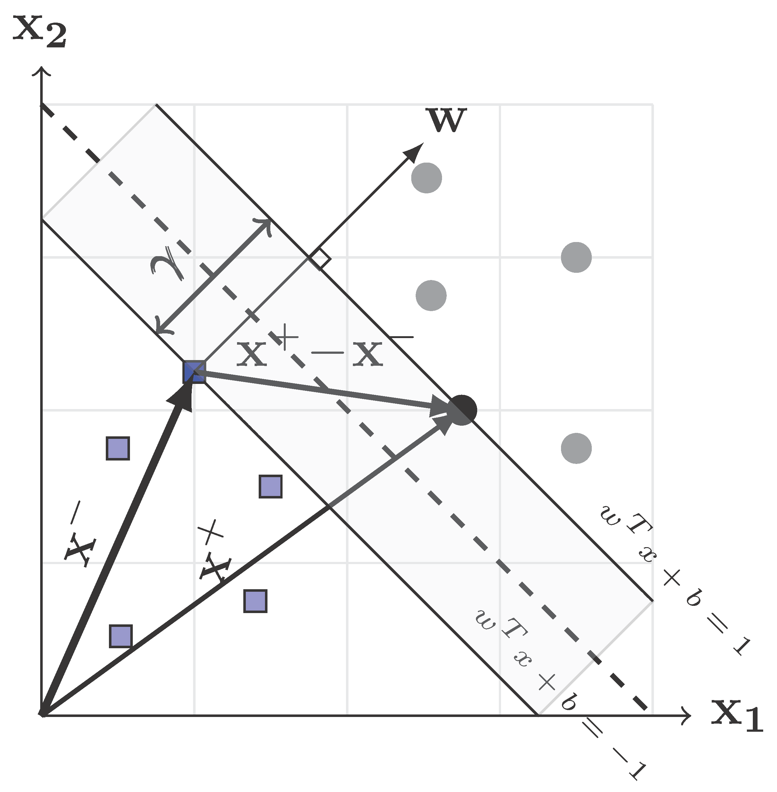
in which denotes the normal vector to the Hyperplane, and b is the bias. A higher number of dimensions, n, leads to a more complex hyperplane. The solution is to find values for and b, in order for the hyperplane to be used to assign new objects to the correct classes. The hyperplane with the largest object-free area is considered the optimal solution, cf. Figure 1.
Considering two support vectors, and , belonging to classes and , respectively, one can show that the margin is the projection of the vector on the normalized vector , i.e.:
Since and , Equation (2) yields in:
In which, the second norm is . The margin is a function of and, thus, the maximum margin solution is found by solving the following constrained optimization problem:
The constraint holds for each training sample closest to the hyperplane (support vectors). In order to solve this constrained optimization problem, it can be transferred to an unconstrained problem, by introducing the Lagrangian function . The primary Lagrangian, with Lagrange multiplier, , is given by:
The Lagrangian should be minimized, with respect to and b, and maximized, with respect to . The optimization problem is a convex quadratic problem. Setting yields the optimal value for the parameters, i.e.:
Substituting for and considering in Equation (6) gives the dual representation of the maximum margin problem, which depends only on the Lagrange multipliers and is to be maximized w.r.t, :
Note that the dual optimization problem depends only on linear combinations of training points. Furthermore, Equation (8) characterizes the support vector machine, which gives the optimal separation hyperplane by maximizing the margin. According to the Karush–Kuhn–Tucker (KKT) conditions, the optimal point ( , ) is achieved for each Lagrange multiplier . Support vectors are those corresponding to . Since, for all sample data out of , the corresponding , the optimal solution depends only on few training points, the support vectors. Having solved the above optimization problem for finding values of , the optimal bias parameter is estimated [19]:
in which is the total number of support vectors. Giving the optimal value of parameters, and , the new data is classified by using the prediction model, , as:
2.2. Nonlinear SVM
The above described SVM classifies the data using a linear function. However, this is only practical if the underlying classification problem is also linear. In many applications, however, this is not the case. The training samples are not strictly linearly separable in reality. This may be due to measurement errors in the data or the fact that the distributions of the two classes naturally overlap. This is achieved by transforming the data into a higher-dimensional space, in which one hopes for a better linear separability. A nonlinear functional is used to map the given feature space into a higher dimension space , by embedding the original features so that:
Accordingly, the scalar product in Equation (8) is replaced by a scalar product of in the new space of . Defining the new space as , the transformed linear hyperplane is then defined as:
Thus, defining the new observables of the data, the SVM algorithm learns the hyperplanes that optimally split the data into different classes using the new space. The steps described above for the linear SVM can then be used here again. The major issue, however, is that the number of components in the nonlinear transformation increases extremely. Particularly, the large number of additional features leads to the curse of dimensionality. This yields an inefficiency of the method, in terms of computational time. The kernel trick solves this issue, as described below.
Kernel Trick
For the non-linear classification, the so-called kernel trick is used, which extends the object area by additional dimensions (hyperplanes), in order to map non-linear interfaces. The most important feature of the kernel trick is that it allows us to operate in the original feature space, without computing the new coordinates in a higher dimensional space. In this context, the kernel trick is used, owing the fact that a linear SVM is constructed for nonlinear SVM. The kernel function is then defined as:
The selection of the most suitable kernel depends heavily on the problem and the data available. A fine-tuning of the kernel parameters is a tedious task. Any functions whose Gram-matrix is positive-definite can be used. The polynomial function with parameters a and d and the radial basis function with parameters are two well-known kernel functions, which satisfy this condition:
A cross-validation algorithm is then used to set the parameters. By assigning the parameters with different values, the SVM classifier achieves different levels of cross-validation accuracies. The algorithm then examines all values to find an optimal point that returns the highest cross-validation accuracy. In the absence of expert knowledge, the choice of a particular kernel can be very intuitive and straightforward, depending on what kind of information we are expecting to extract about the data. In the lake of any information, the first attempt is to try the linear kernel .
2.3. Numerical Algorithm
The numerical procedure employed for the simulation is given in Algorithm 1. As stated, the data set includes the first N vibration modes for damaged and undamaged samples, i.e., , with and as the ith-mode natural frequency of undamaged and damaged samples, respectively. The numerical process of the nonlinear SVM is started with the pre-processing of the data, e.g., normalization the frequencies of all modes in the range of . A minimization process is performed to finding the optimal value of parameters of kernel functions. For that, the absolute minimum distance between the normalized frequencies are used. Once parameters of the kernel are identified, and the non linear SVM is applied for classification. The process ends then for classifying new data.
| Algorithm 1: Numerical procedure for classification using nonlinear SVM. |
 |
3. Numerical Results
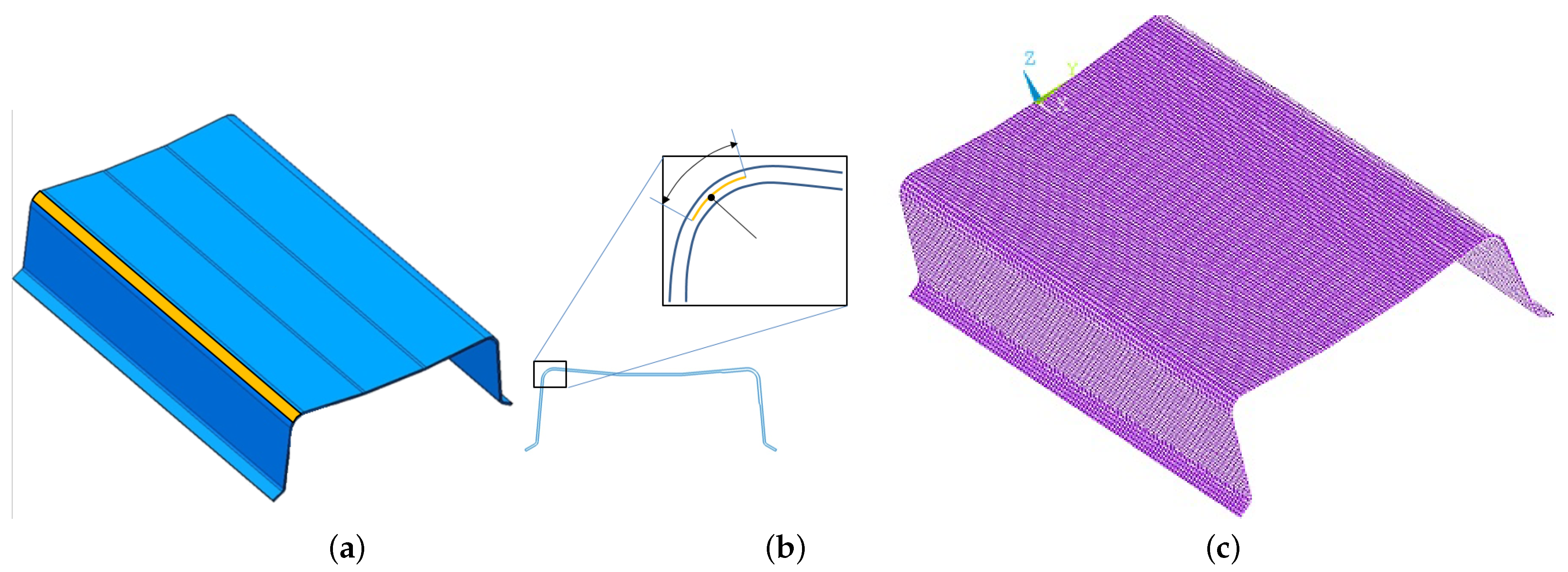
To demonstrate the feasibility of the proposed method, sample components of damaged and undamaged fiber-reinforced composites are assumed to be tested by the experimental modal analysis for identifying the eigenfrequencies. Such a classical experimental procedures is explained in [3], where, to realize the delamination in the damaged samples, very thin plastic foils are artificially implemented between the layers along the fibers, cf. Figure 2.
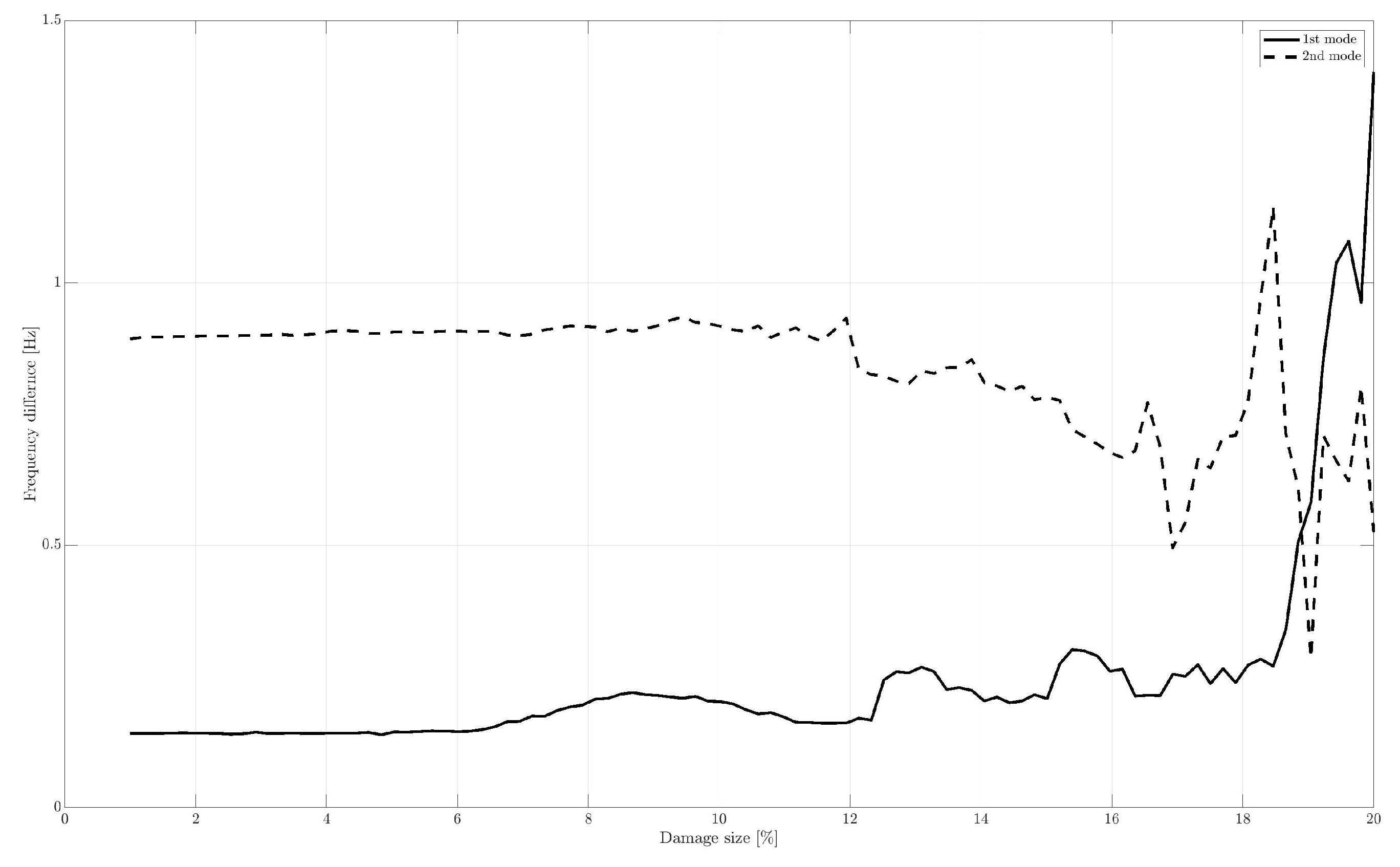
The position of the artificial delamination is shown in Figure 2b. The FEM model in Figure 2c, with and without delamination, is employed for extraction of the training data. To investigate the impact of delamination size on the natural frequencies, various foil lengths are considered. The results are shown in Figure 3.
As shown, for various sizes of delamination (in % of the component length), the frequency differences are very slight. The difference is remarkable for large delamination sizes, particularly, for the 2nd vibration mode. Considering this, any conventional classification procedure cannot be utilized for detection the damaged and undamaged samples. The results are shown Figure 4 for the first 25 natural frequencies of a total of 100 damaged and undamaged specimens from the FEM simulation in for the original feature space .
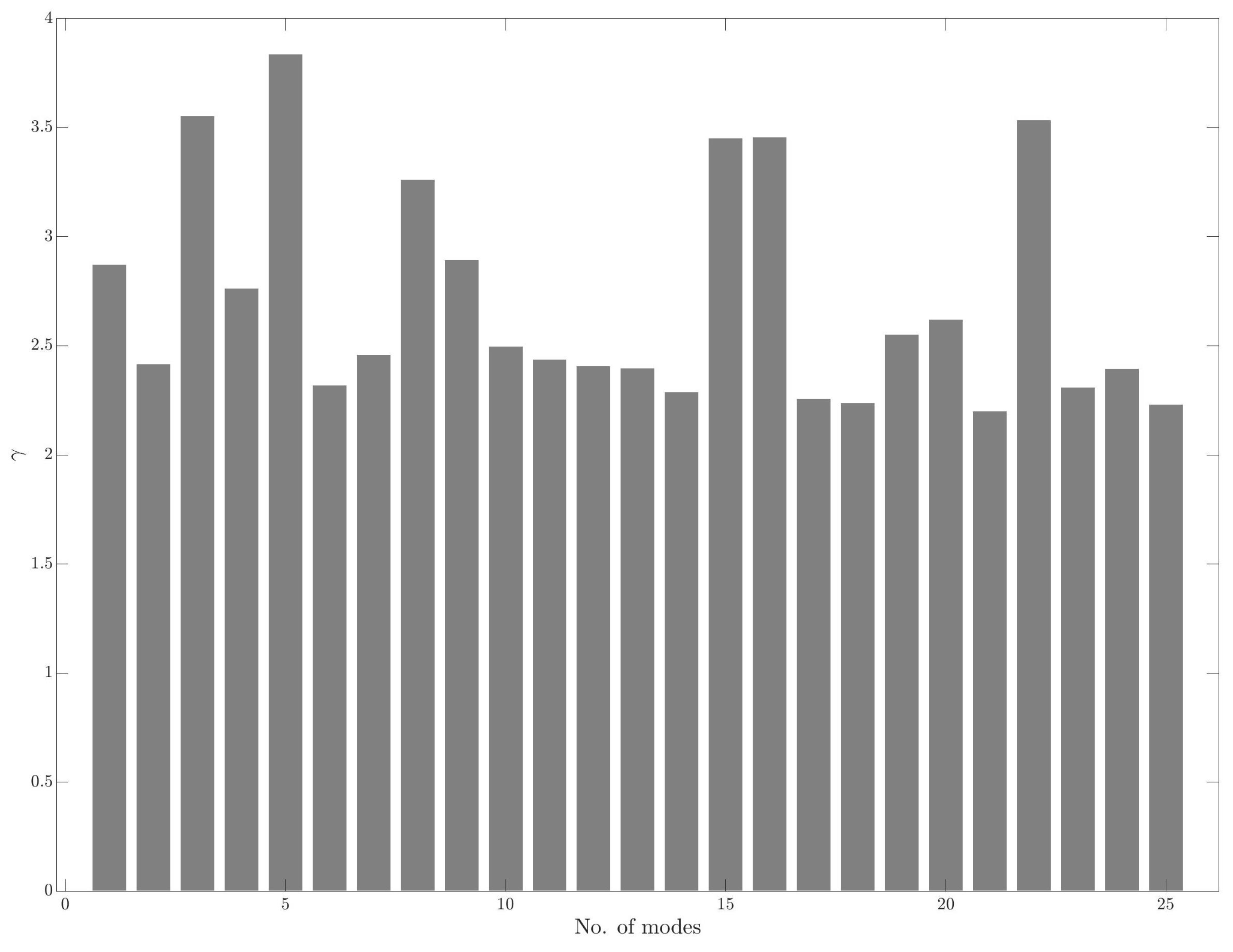
The SVM algorithm seeks for the optimum value of the parameter for the kernel in Equation (17). A custom kernel with free parameters is chosen. The cross-validation search procedure consists of a heuristic line search to determine a promising parameter for each mode. The trend process for all vibrational mode is shown in Figure 5.
As shown, the minimum value of gamma is achieved for mode 21. This ensures the maximum distance for other modes when the kernel is used in classification of the given original features, .
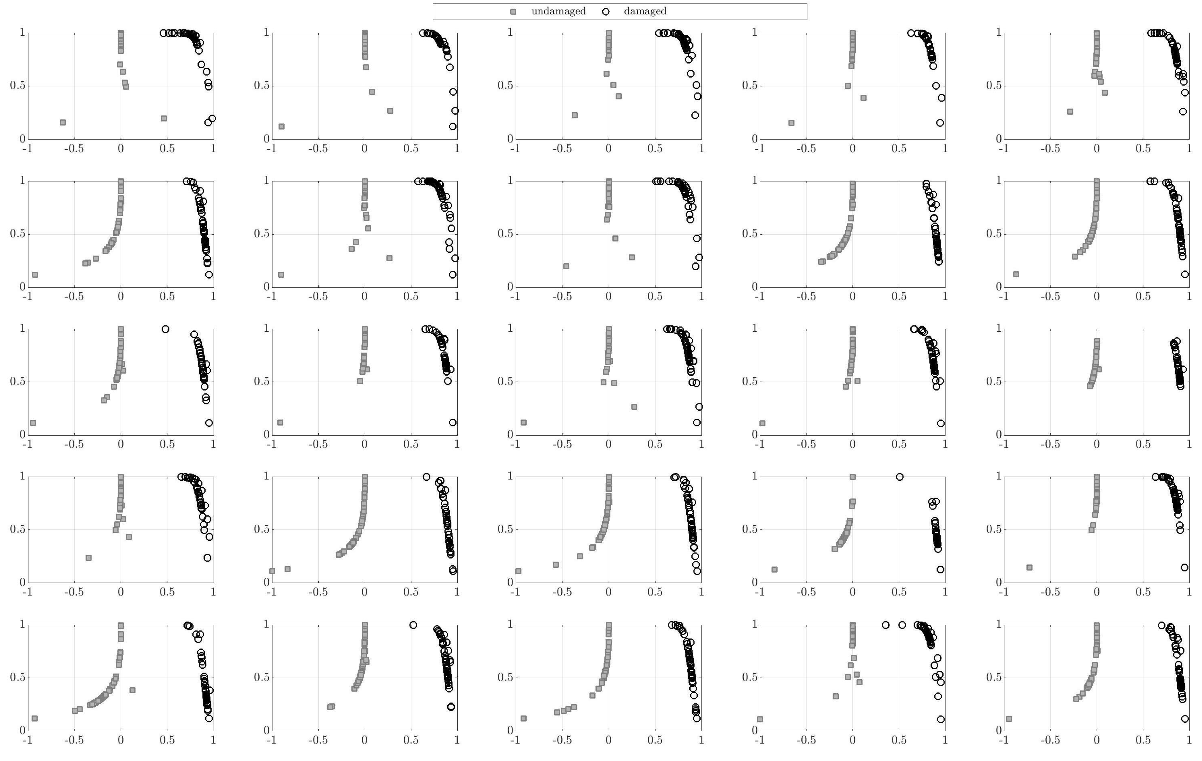
Once the parameters are set, the nonlinear SVM is applied to classify the samples. To this end, two classes are defined, class for damaged and class , for un-damaged samples. A custom function that accepts matrix of feature space as inputs is defined where the Gram matrix using the defined kernel is calculated. The training process uses fitcsvm function in Matlab where an SVM classifier using the defined kernel is employed. This returns a classification SVM model that uses the best estimated feasible point. The best estimated point is the set of parameters that minimizes the upper bound of the cross-validation loss based on the underlying kernel. The results are shown in Figure 6.
As expected, the method results in a large intraclass distance between features to identify classes with very similar values in the dataset, i.e., a small interclass distance.
4. Conclusions
Damage detection methods employing natural frequencies have been extensively investigated using various machine learning algorithms. However, not much attention has been paid to cases where small interclass distance. This is particularly the case with lightweight structures, such as fiber-reinforced composites. The nonlinear SVM machine has been proposed for such situations. The method uses a custom-defined kernel function for the classification. The major effort is in setting the parameters for the kernel. In this work, a cross-validation procedure, using random search, has been used. It has been shown that nonlinear SVM, with the kernel trick, yields a clear classification boundary between damaged and undamaged specimens, even for minor variations in natural frequencies.
Funding
This research received no external funding.
Institutional Review Board Statement
Not applicable.
Informed Consent Statement
Not applicable.
Conflicts of Interest
The authors declare no conflict of interest.
References
- Chen, X.; Yang, Z.; Tian, S.; Sun, Y.; Sun, R.; Zuo, H.; Xu, C. A Review of the Damage Detection and Health Monitoring for Composite Structures. J. Vib. Meas. Diagn. 2018, 38, 1–10. [Google Scholar]
- Doebling, S.W.; Farrar, C.R.; Prim, M.B.; Shevitz, D.W. Damage Identification and Health Monitoring of Structural and Mechanical Systems from Changes in Their Vibration Characteristics: A Literature Review; Technical Report 249299; Los Alamos National Laboratory: Los Alamos, NM, USA, 1996.
- Geweth, C.A.; Khosroshahi, F.S.; Sepahvand, K.; Kerkeling, C.; Marburg, S. Damage Detection of Fibre-Reinforced Composite Structures Using Experimental Modal Analysis. Procedia Eng. 2017, 199, 1900–1905. [Google Scholar] [CrossRef]
- Kessler, S.S.; Spearing, S.M.; Atalla, M.J.; Cesnik, C.E.; Soutis, C. Damage detection in composite materials using frequency response methods. Compos. Part Eng. 2002, 33, 87–95. [Google Scholar] [CrossRef]
- Doebling, S.W.; Farrar, C.R.; Prime, M.B. A summary review of vibration-based damage identification methods. Shock Vib. Dig. 1998, 30, 91–105. [Google Scholar] [CrossRef] [Green Version]
- Salawu, O. Detection of structural damage through changes in frequency: A review. Eng. Struct. 1997, 19, 718–723. [Google Scholar] [CrossRef]
- Wu, J.; Xu, X.; Liu, C.; Deng, C.; Shao, X. Lamb wave-based damage detection of composite structures using deep convolutional neural network and continuous wavelet transform. Compos. Struct. 2021, 276, 114590. [Google Scholar] [CrossRef]
- Ghiasi, R.; Torkzadeh, P.; Noori, M. A machine-learning approach for structural damage detection using least square support vector machine based on a new combinational kernel function. Struct. Health Monit. 2016, 15, 302–316. [Google Scholar] [CrossRef]
- Yang, B.S.; Hwang, W.W.; Kim, D.J.; Tan, A.C. Condition classification of small reciprocating compressor for refrigerators using artificial neural networks and support vector machines. Mech. Syst. Signal Process. 2005, 19, 371–390. [Google Scholar] [CrossRef]
- Boser, B.E.; Guyon, I.M.; Vapnik, V.N. A Training Algorithm for Optimal Margin Classifiers. In Proceedings of the Fifth Annual Workshop on Computational Learning Theory, Pittsburgh, PA, USA, 27–29 July 1992; Association for Computing Machinery: Melbourne, Australia, 1992; pp. 144–152. [Google Scholar]
- Cortes, C.; Vapnik, V. Support-vector networks. Mach. Learn. 1995, 20, 273–287. [Google Scholar] [CrossRef]
- Worden, K.; Lane, A.J. Damage identification using support vector machines. Smart Mater. Struct. 2001, 10, 540–547. [Google Scholar] [CrossRef]
- Liu, L.; Meng, G. Localization of Damage in Beam-like Structures by Using Support Vector Machine. In Proceedings of the International Conference on Neural Networks and Brain, Beijing, China, 13–15 October 2005; Volume 2, pp. 919–924. [Google Scholar]
- Matic, D.; Kulic, F.; Pineda-Sánchez, M.; Kamenko, I. Support vector machine classifier for diagnosis in electrical machines: Application to broken bar. Expert Syst. Appl. 2012, 39, 8681–8689. [Google Scholar] [CrossRef]
- HoThu, H.; Mita, A. Damage Detection Method Using Support Vector Machine and First Three Natural Frequencies for Shear Structures. Open J. Civ. Eng. 2013, 3, 104–112. [Google Scholar] [CrossRef] [Green Version]
- Finotti, R.P.; de Souza Barbosa, F.; Cury, A.A.; Gentile, C. A novel natural frequency-based technique to detect structural changes using computational intelligence. Procedia Eng. 2017, 199, 3314–3319. [Google Scholar] [CrossRef]
- Viitaniemi, V.; Sjöberg, M.; Koskela, M.; Ishikawa, S.; Laaksonen, J. Chapter 12—Advances in visual concept detection: Ten years of TRECVID. In Advances in Independent Component Analysis and Learning Machines; Bingham, E., Kaski, S., Laaksonen, J., Lampinen, J., Eds.; Academic Press: Cambridge, MA, USA, 2015; pp. 249–278. [Google Scholar]
- Crammer, K.; Singer, Y. On the Algorithmic Implementation of Multiclass Kernel-Based Vector Machines. J. Mach. Learn. Res. 2002, 2, 265–292. [Google Scholar]
- Bishop, C.M. Pattern Recognition and Machine Learning; Springer: New York, NY, USA, 2006. [Google Scholar]
Figure 1.
Two-dimensional hyperplane (dashed line) in the SVM, with support vectors and , belong to both classes.
Figure 1.
Two-dimensional hyperplane (dashed line) in the SVM, with support vectors and , belong to both classes.

Figure 2.
(a) Sample composite component with artificial delamination, (b) the position of delamination, (c) FEM model for data generation.
Figure 2.
(a) Sample composite component with artificial delamination, (b) the position of delamination, (c) FEM model for data generation.

Figure 3.
The impact of delamination size on frequency difference of damaged and undamaged samples for the 1st and 2nd modes.
Figure 3.
The impact of delamination size on frequency difference of damaged and undamaged samples for the 1st and 2nd modes.

Figure 4.
The first 25 eigenfrequencies, [Hz], for damaged and undamaged samples are slightly different and not linearly separable (horizontal axis: no. of samples).
Figure 4.
The first 25 eigenfrequencies, [Hz], for damaged and undamaged samples are slightly different and not linearly separable (horizontal axis: no. of samples).
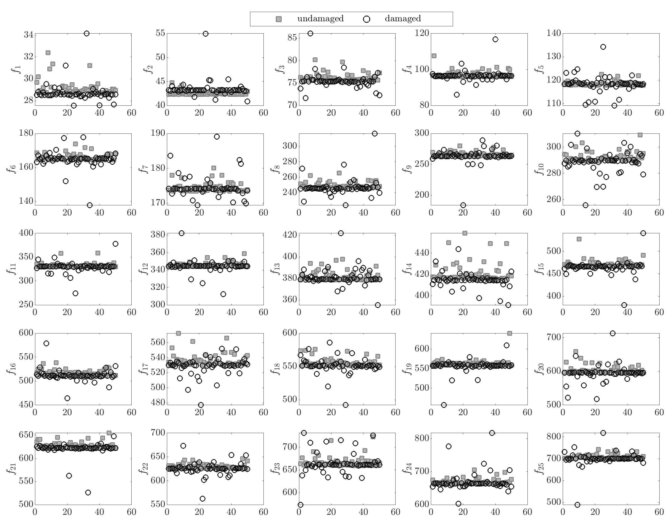
Figure 5.
Optimum values of the kernel parameter for each vibration mode.

Figure 6.
Classification of the damaged and undamaged components using the kernel trick.
Publisher’s Note: MDPI stays neutral with regard to jurisdictional claims in published maps and institutional affiliations. |
© 2021 by the author. Licensee MDPI, Basel, Switzerland. This article is an open access article distributed under the terms and conditions of the Creative Commons Attribution (CC BY) license (https://creativecommons.org/licenses/by/4.0/).
Share and Cite
MDPI and ACS Style
Sepahvand, K.K. Structural Damage Detection Using Supervised Nonlinear Support Vector Machine. J. Compos. Sci. 2021, 5, 303. https://doi.org/10.3390/jcs5110303
AMA Style
Sepahvand KK. Structural Damage Detection Using Supervised Nonlinear Support Vector Machine. Journal of Composites Science. 2021; 5(11):303. https://doi.org/10.3390/jcs5110303
Chicago/Turabian StyleSepahvand, Kian K. 2021. "Structural Damage Detection Using Supervised Nonlinear Support Vector Machine" Journal of Composites Science 5, no. 11: 303. https://doi.org/10.3390/jcs5110303