Exploring the Spatial Variations of Stressors Impacting Platform Removal in the Northern Gulf of Mexico

Abstract

Although progress has been made to advance our understanding of the risks involved in offshore oil extraction activities, a regional scale understanding of factors contributing to losses in infrastructure integrity are lacking. Recent data integration efforts have resulted in a comprehensive database that allows for an unprecedented study of the external and internal factors that impact the structural and operational integrity of offshore platforms in the Gulf of Mexico. This study constitutes some of the initial explorations into that database by focusing on the relationships among a diverse set of variables and the age at which a platform is removed. We apply Geographically Weighted Regression to account for the heterogeneity of the operating environment, finding robust yet unexpected relationships that shed light on some of the factors that influence platform removal. Our findings pave the way for future studies aimed at building actionable knowledge.

1. Introduction

The majority of offshore oil platforms have an operational design life of 20 to 30 years. Currently, more than 60% of the operating platforms in the Gulf of Mexico (GoM) were installed more than three decades ago [1,2]. Part of the reason for this extension in operating life comes from advances in reconstruction, repair, and retrofitting techniques on the platforms. Another reason is that extending the operating life is economically attractive [3]. Increasing the time that existing infrastructure remains operational will eventually reduce costs while maximizing energy production and profit. It may also play an important role in converting these structures to meet renewable energy demands. This has been a trend since the onset of offshore energy exploration and development [4]. Engineering advancements have contributed to a higher production potential, but also to the need for more research on structure design and knowledge gaps [5]. Generally speaking, platform life extension depends heavily on proactive maintenance and monitoring to reduce the risk that critical components fail, resulting in a loss-of-control event [5,6].

Offshore platforms are subject to various stressors over time. These can be endogenous (coming from the platform itself) or exogenous (coming from external forces) and together will contribute to a decline in the integrity of a platform. The result of such declines in integrity can result in more frequent maintenance, decreases in production, leaks, and equipment failure. Where the latter is concerned, the key to ensuring that equipment does not fail is a robust maintenance and monitoring strategy, the lack of which has been found to be the leading cause of infrastructure failure [7]. Similarly, Halim et al. [8] noted that inadequate (or complete lack of) maintenance was the leading cause of offshore platform incidents involving fires, personal injury, structural breaks, spills, and blowouts.

While advances in structural integrity monitoring, maintenance system management, and risk mitigation strategies are evolving [9,10,11], it is important to acknowledge that stressor associated with declining integrity continue to emerge. Some of these stressors are well known. For example, the fatigue generated by repeated wind, wave, and currents has prompted changes to design standards over time [12,13]. More recent work makes the connection between environmental loadings and the risk of incidents or failure even more explicit [9,14], with particular attention focused on the effects that extreme weather events have on offshore platforms and their associated design standards [15]. Still, many platforms currently operating in the GoM were designed more than three decades ago and recent studies suggest they may be more susceptible to failure during extreme weather events, especially in the presence of corrosive effects or environmental loadings that may have a decreased structural integrity [16,17].

To date, techniques to understand infrastructure integrity have typically focused on individual structures or lease blocks rather than a general region-wide approach [18,19]. The absence of a geographically broad approach is partly due to the lack of complete data sets on the operating environment of offshore infrastructure. However, with the advent of big data collection strategies, along with increased access to information about production and environmental conditions, there is an opportunity to leverage new data to discover regional trends related to variations in infrastructure integrity.

In an effort to develop a deeper understanding of the factors that impact the integrity of platforms, we integrate datasets spanning structural characteristics, incident history, environmental variables, and production records. We then use singular value decomposition (SVD) as a variable selection technique for Geographically Weighted Regression (GWR) to account for the potential variation in spatial trends across the study region, while assessing the relationship between platform stressors and platform removal age [20]. Our evaluation provides several key insights for regulators, operators, and responders. First, this work evaluates the differential effects of endogenous and exogenous stressors on platform integrity. Second, it supports industry–government interactions and decision making with enhanced maintenance and inspection strategies to reduce the risk of failure. Third, the ability to relate the effect of stressors on integrity to a specific location (i.e., platform) serves as an important step towards preemptive maintenance strategies. Lastly, although some studies have previously been completed [21,22], few have taken a system-wide explanatory approach. Correspondingly, the conceptual framework of this approach and spatial analyses are generalizable to an array of diverse settings.

2. Literature Review

Since the installation of the first GoM platform in 1938, which was erected in 14 feet of water about a mile offshore, continual advances in manufacturing and development have enabled a steady progression of offshore production and exploration in deeper water and drilling depths [23]. In the GoM, more than 70 platforms operate in ultra-deepwater environments at depths of more than 5000 feet and target reservoirs several miles under the ocean floor [24]. In addition to managing the structural fatigue associated with the extreme pressure and temperature of the materials in the targeted reservoirs, there are a variety of environmental factors that may compound the stress caused by the normal wear and tear of daily operations. Industry and government regulators are aware of the stress caused from operation in offshore environments [25], which have been exacerbated by an increase in extreme weather over the past decade. These realizations support recent research towards identifying and mitigating the impacts of operations in marine environments [26].

When it comes to analyzing the factors effecting the operation of offshore structures, industry experts and researchers commonly focus on the concept of structural integrity [27]. In this context, an energy infrastructure system of high integrity is one where the systems of components that make up the macrostructures (i.e., platforms) of the offshore system are operating in a way that does not impede production performance. Conversely, a low integrity system is one where changes in the macrostructures begin to impinge on the performance of the system. Indicators of low (or decreasing) integrity can manifest in many ways. For example, platforms may begin to experience an increased rate of equipment failure [8,14], degradation of the key joint welds [28], or noticeable reductions in the strength and ductility of the structure due to pitting [17,29]. The decline and ultimate failure of these components is the leading cause of platform-related incidents including spills, blowouts, injury, and loss of life [7,8].

2.1. Factors Affecting Platform Integrity

Previous work suggests that declines in platform integrity can come from many sources, which include external corrosion, structural stress from the surrounding environment, incident history, and production operations [9,14,27,30]. Although all these sources can decrease structural integrity, some may contribute more prominently than others and vary in their effects across the GoM.

2.1.1. Platform Design and Production

The design life of an offshore platform is defined as “the assumed [time] period for which a structure is to be used for its intended purpose with anticipated maintenance but without substantial repair from aging processes being necessary [31]”. Generally, the design life of offshore oil and gas platforms ranges from 20–30 years. Globally, 30% of the approximately 6500 platforms operating in the offshore environment have been in operation for more than 20 years and are near or past their design life [32]. The largest portion of those platforms operate in either the GoM or the North Sea [2,33,34]. However, offshore infrastructure operating beyond its design life is also observed in other offshore plays [35,36].

The platform installation year has been found to be a strong predictor of integrity [2]. As platforms age, the effects of fatigue and corrosion increase, leading to degradation, unless actively managed [2,9,37,38]. Platform age has been associated with heightened levels of equipment failure, corrosion, and incidents. For example, a recent report identified a positive relationship between platform age and incidents, equipment failure, and corrosion resulting from factors that are external to the platform, including the continuing exposure to weather [39]. This was further supported in a study by the National Oil Spill Detection Response Agency in Nigeria, where they found that production on infrastructure past its design life is a possible factor in oil spill incidents [40]. Related to this, stressors from daily operations on platforms, such as production, accumulate over time. If not addressed through maintenance the stress may result in heightened structural fatigue and ultimately a decrease in integrity. In fact, a recent study suggests that platforms processing greater production volumes over longer periods of time are associated with a higher probability of incidents [38].

Offshore platforms are classified as either major or non-major structures. Major structures contain at least six completions, or more than two pieces of production equipment [1]. Major structures have a slightly lower design life than non-major structures [41], which might be attributed to the increased operational wear-and-tear of production from more completions. That said, the design codes for major and non-major structures have become more rigorous over time by adapting to the increase in production intensity and weather events, such as higher wave heights and stronger wind speeds [2,9,42]. Changes to design codes have resulted in taller deck heights, updated safety systems, and reinforced welding requirements. Importantly, design codes differ for major and non-major structures and various platform structure types. In addition, fixed platforms are affixed to the seafloor, making them stationary, and are more susceptible to waves than mobile platforms due to their rigidity [42].

2.1.2. Metocean

One of the most likely factors contributing to structural fatigue and associated declines in integrity comes from ambient oceanographic and weather-related events [43]. Environmental loads include wind, waves, and currents, which are exasperated in the presence of hurricanes and tropical storms. In 2005, hurricanes Katrina and Rita destroyed 115 platforms and damaged 52 others [44]. Three years later, hurricanes Ike and Gustav impacted operations on approximately 2127 platforms, destroyed 60 platforms, and caused extensive damage to 31 platforms [45]. More recently, hurricane Laura shut-in almost half of the offshore operating platforms in 2020, stopping production for 15 days and reducing production by approximately 14.4 million barrels [46]. Enhanced loadings from increased wave height and currents are of particular interest, but high wind speeds can also contribute to fatigue and, albeit gradually, to structural components [14]. In the context of climate change, we can expect that the structural loadings associated with oceanographic and weather-related events will increase. For example, recent work [47,48] found that climate change will result in larger extreme wave events in the northern Gulf of Mexico, causing current design-criteria estimates to be unsafe in the near future.

While the immediate and deleterious consequences of weather events for some platforms operating in the GoM are known, other metocean conditions are less well understood, but can fatigue a structure over time [9,14]. Such metocean conditions include temperature and currents or biologic measurements of nitrate, salinity, and concentrations of other nutrients that, when combined, may enhance the corrosion of an offshore structure, or promote marine growth [16,17]. Corrosion can affect properties such as strength and ductility under certain environmental conditions [29] and may be exacerbated by changes in the water column. Specifically, water temperature, depth, and current velocity can contribute to higher rates of corrosion. Bhandari [29] and Nunez [49] both found increased corrosion rates with higher water temperatures, while Guedes Soares et al. [50] and Melchers [51] reported positive correlations between surface velocity and the rate of pitting corrosion. Water depth appears to also correlate with corrosion; however, it can be difficult to disentangle depth from other factors that vary with water depth and influence corrosion such as oxygen concentration, temperature, steel type, pollution, salinity, and water velocity [29]. The work by Muehlenbachs et al. [38] and Shultz and Fischbeck [52] suggest that operational water depth may be associated with higher reported incident rates, potentially signaling declines in integrity that go beyond just the corrosive effects.

2.1.3. Geohazards

Production platforms are connected to other forms of infrastructure, including wells that go into the subsurface and pipelines that traverse or are buried beneath the seafloor. Past incident reports and studies have shown that geologic conditions and associated geohazards can have a considerable impact on platform operational abilities. Reported geohazards include mudslides, subsidence, and problematic reservoir conditions [53,54,55,56,57]. Problematic reservoir conditions include those with abnormal or high-pressure high-temperature environments that might result in kicks during drilling, which have led to blowouts. These incidents most commonly occur during the exploratory drilling phase [53]. As evidenced by the Deepwater Horizon disaster, blowouts can impact the surrounding environment as well as associated infrastructure [58].

2.1.4. Incidents

As noted by [8,14], incidents relating to structural fatigue, material degradation, and other incremental damages over time can lower the structural integrity of platforms. Incidents might represent human error, a build-up of structural stress from day-to-day operational wear-and-tear, constant environmental stressors, or extreme weather events [30]. Reported incidents include injuries, fatalities, fires and explosions, leaks and spills, blowouts, loss of well control, and collisions [24] and may suggest latent indicators of declining integrity [9,14] and equipment dependability.

2.2. Existing Methods of Integrity Evaluation

A series of frameworks have previously been proposed (some implemented) to monitor and manage integrity. One of the main approaches to this is the structural integrity management (SIM) approach which considers stressors including environmental loadings and accidents to assess the life cycle status of a structure. SIM aims to reduce the impact of stressors by slowing structural fatigue and maintaining or increasing operational capabilities [9,10,11]. SIM and other life cycle analytical strategies have been adapted to incorporate stress from additional features, such as the application of corrosion models to predict fatigue life on jacket structures [37]. However, these evaluations typically focus on one structure at a time and are highly dependent on accurate and consistent inspection records, which tend to be lacking with older platforms [27].

Past studies have incorporated additional monitoring techniques such as key performance indicators (KPIs), qualitative and quantitative risk assessments, and intelligent modeling methods to fine tune management programs and routine inspection schedules and techniques [14,59,60,61]. For example, Sharp [14] developed KPIs for fixed and mobile platforms to identify hazards and linked incident events. Guédé [59] took a related approach by integrating American Petroleum Institute (API) guidelines with design criteria, structural conditions, and modifications to produce global and local risk assessments for fixed offshore structures. These studies underpin the importance of incorporating environmental stressors, but again, are applied at the individual platform-level, which obfuscates regional trends.

At a regional scale, the stress on platforms from exogenous and endogenous factors likely varies spatially and temporally. Interestingly, only a few studies have taken a spatially explicit approach to catalog these variations. The study by Liu et al. [62] is one example where they analyzed the platform status for both federal and state waters of the northern GoM using a time-series analysis of 26,000 remotely sensed images between 1982 and 2017. Muehlenbachs [38] also applied a temporal analysis of platform incidents using data from the GoM from 1996 to 2010. They applied a logistic regression model and found a positive correlation between water depth and the likelihood of incident reports. Other work focused on infrastructure (albeit onshore) utilized hotspot analysis to understand water infrastructure failure with data that varied over space and time [63].

Clearly, in a situation where data are likely to vary across space or time models that produce single coefficients to represent what happens on average cannot adequately capture the relationships between variables at a local level. For these situations, methods that can capture variations over space to reflect local nuances are beneficial. One such approach is GWR, which has been widely applied to account for local variations in data related to health and pollution [64], the distribution of environmental amenities [65], and road tanker accident patterns in Nigeria [66]. GWR utilizes a modified regression framework to consider changes in relationships across multivariate data sets [67] and in doing so overcomes some of the limitations of “global” regression models that only produce single regression coefficients (i.e., least squares or simultaneous autoregression) [68]. That said, GWR is still susceptible to some of the limitations of regression, including multicollinearity among independent variables [69]. GWR has yet to be applied to understand the spatial relationships between stressors on offshore infrastructure.

3. Materials and Methods

The GoM is a heterogeneous setting with many environmental and geologic factors that can contribute to differences in the rate of fatigue, stress, and hazard potential. These stressors, as well as production and technological advances in design and fabrication, impact the integrity and associated lifespan of offshore infrastructure. Previous studies have applied monitoring or assessment frameworks on a platform-level basis or have used methods that evaluate regional trends in platform integrity on average. In this work, we utilize GWR to explicitly consider the inherent variance of factors associated with stress on offshore infrastructure. In doing so, we are able to analyze the local relationships between stressors and integrity. We utilize a unique platform-level data set published by the National Energy Technology Laboratory (NETL, Morgantown, WV, USA) [30,70] containing information on both the endogenous and exogenous factors associated with declines in integrity (Appendix A). We utilize SVD to identify significant variables that strongly covary with our target variable of interest, which informs inclusion of independent variables (stressors) in the GWR model. The resulting GWR model is then used for predicting age at removal.

3.1. Data

This study focuses on offshore platforms operating within the federal waters of the GoM (Figure 1), including those that are currently operating and those that were at one point operating but have since been removed or destroyed (n = 7296). Most of these platforms are fixed structures, though floating platforms such as tension-leg and mobile offshore production units are also included. The data set contained 1225 attributes for each platform that relate to four key stressor categories: structural and production data (64.5%), ambient environmental conditions (platform interaction with storm events, proxies for external corrosion, metocean) (17.8%), platform-specific incident history (15.1%), and geohazards (2.6%). As detailed in Nelson et al. [30], attributes were created by spatially extracting the original data (Appendix A) to each platform’s location [30]. Moreover, statistical attributes representing temporally dynamic data (i.e., ambient environmental conditions) were calculated using only data that occurred during each platform’s lifespan.

The data set was split into two subsets according to whether the platform was removed or currently operating. Removed platforms contained a known removal date or a recorded destroyed date within the incident records. This subset was used to develop the explanatory GWR model and to assess measures of model fit and performance. The second set contained the currently operating platform in the GoM, which lacked a removal date and not marked as destroyed in the incident records. After developing the model using platforms that had already been removed or destroyed, we applied it to the second data set that did not have a removal age. This allowed us to evaluate the modeled removal age against the current age of the operating platform to assess the degree to which they are past (or still within) their modeled lifespan.

3.2. Dependent Variable

For this analysis, we operate under the assumption that decreases in integrity will ultimately result in platform removal. Thus, we were interested in the age of the platform at the time it was removed. For platforms where a removal date was known (data subset 1), we subtracted the install date from the removal date to obtain the age of the platform when it was removed (in years). Out of the initial 7296 records, 224 did not have install or removal date and were excluded from the analyses. The final data set contained a total of 7072 platform records (5315 removed, 1757 operating).

3.3. Independent Variable Selection—Singular Value Decomposition

Recall that within the platform data set were platform attributes (stressors) that fell into one of four categories: structural and production characteristics, characteristics of the operating environment, hazards along the seafloor or a subsurface spatially linked to platform operations and infrastructure, and incident history. In total, there were 1225 individual attributes in the data, many being derivatives of one another. As such, there was a high possibility for multicollinearity to affect the modeling process. To reduce multicollinearity of the independent variables, while also retaining interpretability and reducing the dimensionality of the data, we leveraged SVD for variable selection.

SVD is widely used to synthesize information contained in a data matrix. In earth sciences, SVD is often applied to a covariance (or correlation) matrix of environmental observations to understand which variables are related, and to identify which variables may be redundant or less important (uncorrelated). Using SVD to identify the relationships within a covariance or correlation matrix is similar to (and often a part of) Principal Component Analysis (PCA) or Empirical Orthogonal Functions (EOF) [71,72]. At its core, SVD reduces the dimensionality of data by decomposing any data matrix into two orthogonal matrices representing rotations, and a diagonal matrix representing stretching (Equation (1)). The information within any given matrix can be summarized by identifying the directions along which the largest deformation (inherent to the matrix) occurs, given by singular vectors ($U$ and $V$), and the amount of deformation given by the entries of the diagonal matrix ($\Sigma$), the singular values:

$$A=U\Sigma V^T$$

(1)

where $U$ is an m × m matrix of singular vectors and $V$ is an n × n matrix of singular vectors if $A$ is an m × n matrix. $\Sigma$ is an m × n diagonal matrix of nonnegative entries.

When $A$ is the covariance matrix of predictors, the right-hand singular vectors in V identify the variables that best explain the target value (in this case, age at removal). The SVD is effectively a decomposition of a matrix into a sum of rank-one matrices. When applied to the covariance matrix of platform data, each rank-one matrix in its SVD explains a fraction of the total variance in the data set, that fraction is given by the singular value held on the diagonals of ($\Sigma$). When the singular values are placed in descending order (s₁ ≥ s₂ ≥⋅s_min), the first k rank-one matrices from the SVD approximation of the covariance matrix constitute the best possible linear approximation of the covariance matrix—this is the Eckart–Young theorem. Importantly, the Eckart–Young theorem shows that the sum of k rank-1 matrices given by $\widehat{A}$ is the rank-k matrix that minimizes,

$$\left||A-\widehat{A}|\right|$$

(2)

with some suitable norm such as the spectral norm (or two norm) in Equation (2). This approximation provides a reduced-dimension linear approximation of the target variable (one of the columns in $A$) as a combination of the rest of the independent variables. Thus, SVD provides an efficient way to synthesize the information of a data matrix while retaining interpretability. It allows us to identify the relationships between variables, the presence of multicollinearity within the data, and to identify the variable signaling the strongest relationship with the target variable. It also provides a selection criterion to discard variables that do not contribute to the linear approximation of the target variable. It should be noted that SVD, like PCA and other factor analysis methods, are data reduction strategies. This means that some data and information will be left out as a result of the approximation. That said, it is the aim of data reduction to identify the most meaningful information as possible, while removing redundant or noisy information.

Considering the diverse nature of what the data represented (e.g., environmental metrics, incident counts, water depths), numeric values were standardized using z-score standardization. This accounted for the various scales inherent in the data (which is useful for SVD) and was also used for GWR to interpret variable importance. Records containing missing values were filled prior to standardization using k-nearest neighbors (KNN) imputation [73].

Rather than evaluate the entire set of data at once, we began by dividing and grouping the attributes into their four categories (and some subcategories). For example, all metocean attributes were separated out from the larger data set and split into three subcategories: ambient data, storm series data, and proxies for external corrosion. Next, we applied SVD to each of the covariance (or correlation) matrices representing these reduced data sets, each time identifying the variables explaining the largest fraction of the total variance of the target variable from the subset of data. The selection of these variables served as our independent variables. Following this initial selection, final SVD decompositions were used to select the set of variables that best explained the age of removal as a linear combination.

3.4. Geostatistical Analysis and Prediction

The GWR analysis proceeded in two phases. We first developed and tested the model using the subset of platforms that have already been removed from operation in the GoM. We established model fit, explanatory power, and accuracy of predictions using a train-test (80%/20%) split of these data. Next, we applied the model to platforms currently operating in the GoM to estimate the age at which each of these platforms should be removed based on the model of when other platforms were removed. The GWR method uses a spatially explicit approach to account for variations in relationships between independent and dependent variables across a large region. Formally, GWR is represented as:

$$y_i={\beta }_o+{\displaystyle \sum }_k{\beta }_k\left(u_i,v_i\right)x_{ik}+{\epsilon }_i,$$

(3)

where $x_{ik}$ is the $k$th predictor variable, ${\beta }_k$ is the $k$th coefficient at location $\left(u_i,v_i\right)$, and ${\epsilon }_i$ is the error term [67]. The model considers the variation in spatial pattern by estimating a unique regression model at each $i$th observation using the relationship between independent and dependent variables in a neighborhood surrounding that observation. The model weighs these observations such that the values nearest them will receive a higher weight than those observations that are further away. The spatial structure of a given region determines the size of the neighborhood used to estimate the coefficient values. This is calibrated with a distance-weighted kernel $\left(d\right)$. For these data, the variation in distance between observations necessitates the use of an adaptive bi-square kernel where the size of the kernel (bandwidth) was determined using a “golden search” optimization routine [68]. The final neighborhood size in this analysis was 126.

All processing and analyses were performed in Python using the MGWR (Multiscale Geographically Weighted Regression) and Pysal libraries [68]. We used ArcMap 10.8 [74] to spatially visualize the parameter estimates for each platform, including model diagnostics (local coefficient of determination (R²) and residuals) and the difference between modeled age at removal and current age for the currently installed platforms.

4. Results

We began by applying SVD to reduce the dimensionality of the platform data set while distilling the data down to the key variables that covary with our target variable, platform removal age. We then leveraged the results of SVD to inform our variable selection for GWR.

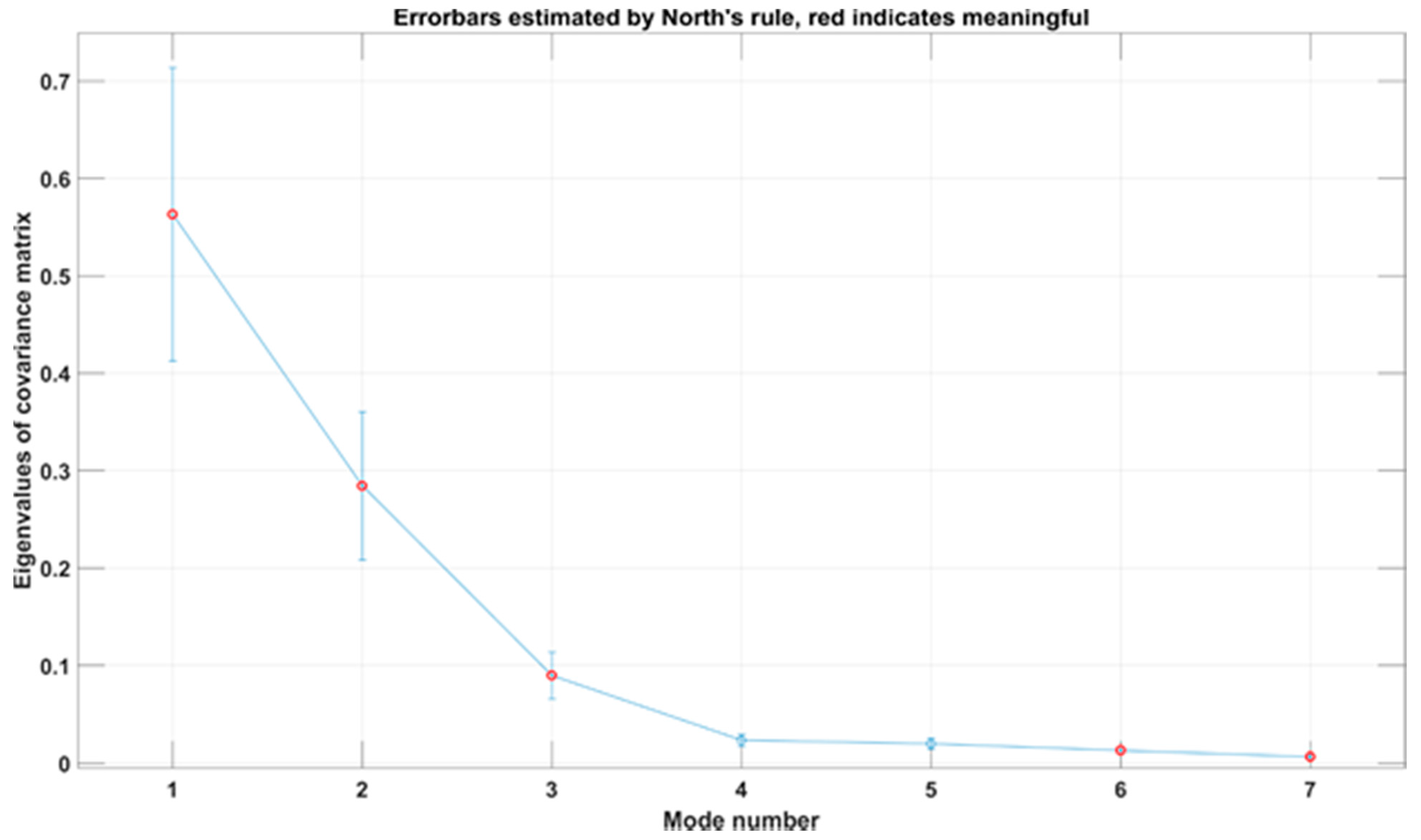
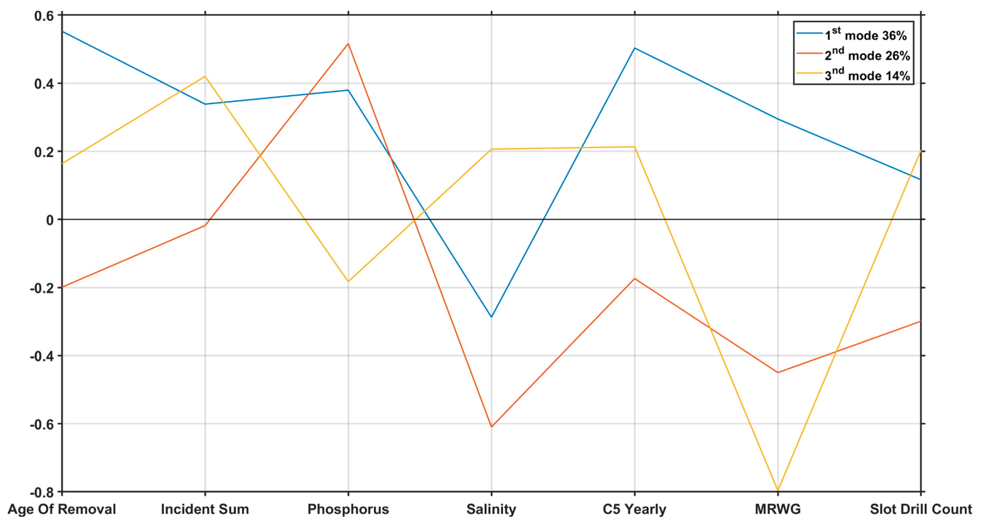
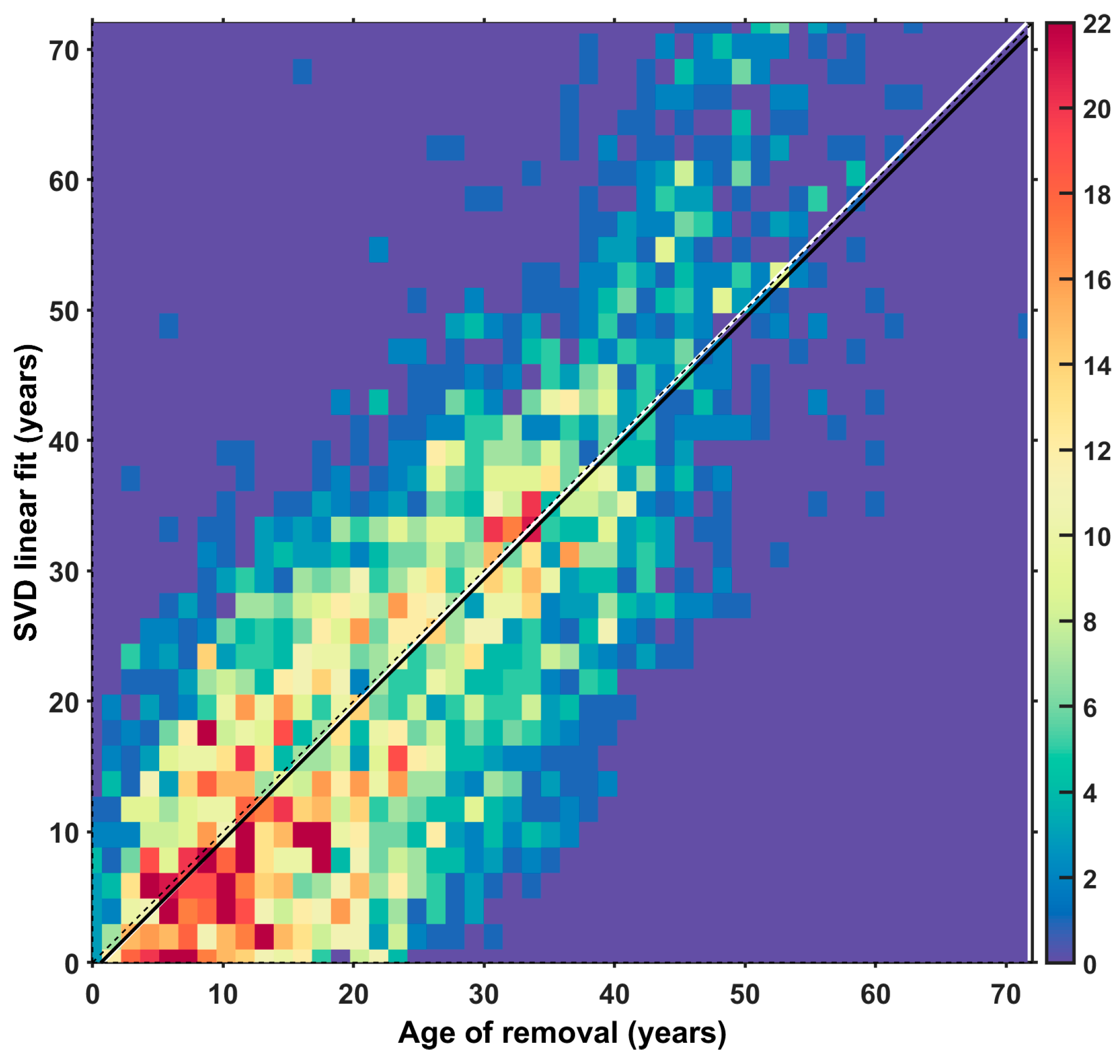
4.1. Singular Value Decomposition

We identified a set of six variables through the SVD procedure that covary with age at removal. The variables were slot drill count, Category 5 hurricane (C5) yearly, maximum reported wind gust (MRWG), salinity, phosphorus, and incident sum corresponding to three singular vectors (Figure 2). Each of the colored lines in Figure 2 correspond to one of the right singular vectors, where the order of the singular vectors (1st, 2nd, and 3rd mode) indicates their importance for describing the information within the data set, accounting for 36%, 26% and 14% of the variance, respectively, for a total of 76% of the variance explained with the first three vectors. The lines’ deviation from zero on the y-axis indicates the variable’s (x-axis) contribution to the singular vector. For example, in the first singular vector (1st mode), incident sum and MRWG explain a large portion of the variance. In the second singular vector (2nd mode), C5 yearly is the most important contributor, but phosphorus and incident sum are also relatively important. In the final singular vector (3rd mode), most of the information is contained in the phosphorus and salinity variables. North’s test [75] was used to confirm that these first three singular values were significant (Appendix B).

The reader may also notice that we included our target variable (age at removal) in the SVD. This allowed us to evaluate whether the variables associated with each singular vector had some level of correspondence with age at removal. If the variables making up each singular vector did not correlate with age at removal, we would expect the point at age at removal to be at or near to zero. The deviation from zero at age at removal for each singular vector indicates there is some linear correspondence between these variables and age at removal. This is further illustrated by the scatter plot in Figure 3. Here, we plotted the SVD linear fit to age at removal where pixel color and associated color ramp provide a visual representation of the underlying plot of points (number of observations) in the scatterplot in which the relationship is made. The SVD linear approximation is a decent predictor of age at removal, with an R² of 0.63, a Pearson correlation of 0.79, and a near normal residual distribution (Appendix C).

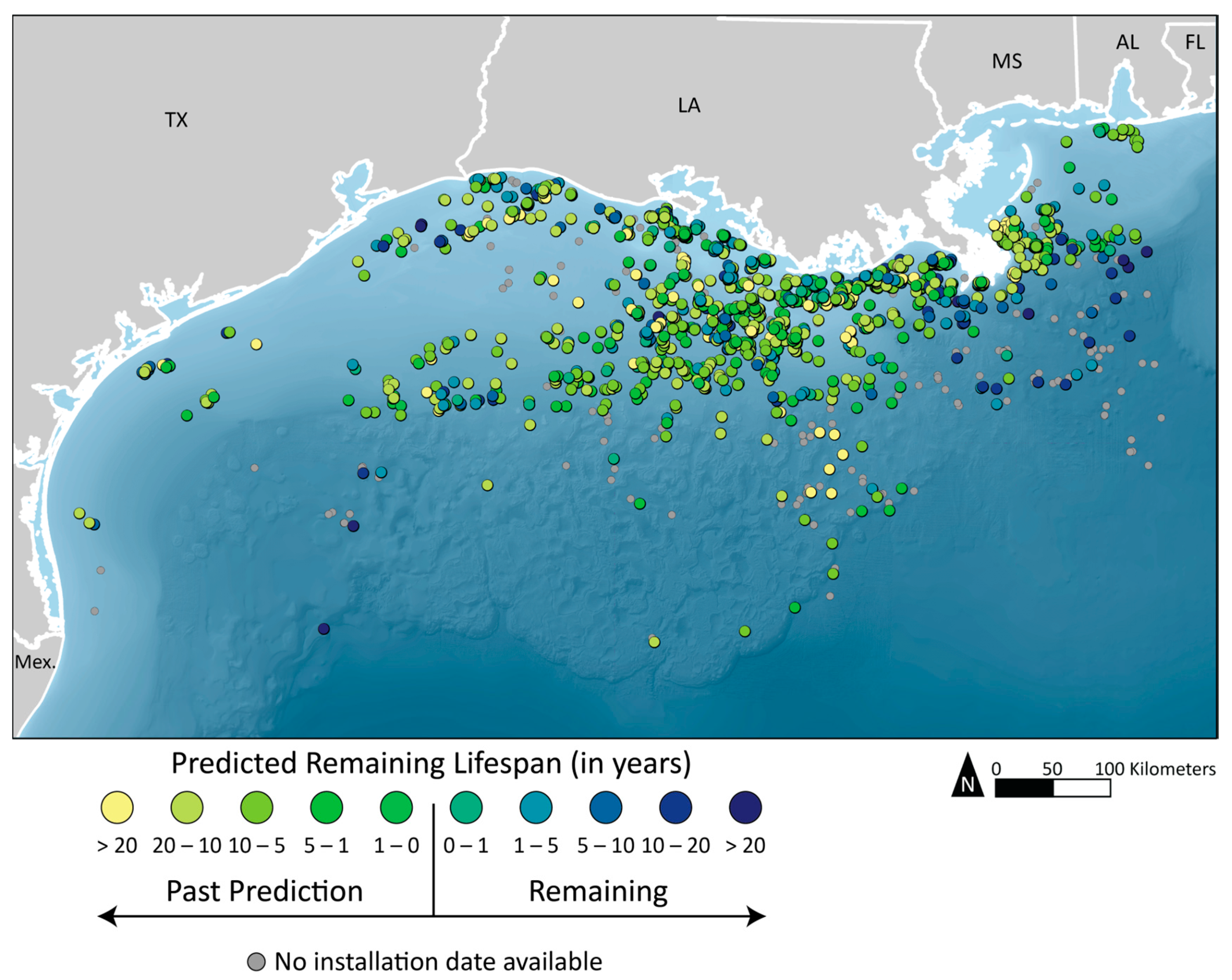
4.2. Geographically Weighted Regression

We began the GWR analysis using the set of variables identified through the SVD. However, after several model runs and diagnostics of model fit, we added two additional variables to the GWR analysis: water depth and surface magnitude. In total, we included eight independent variables in the GWR model (

Table 1. Descriptive statistics for the final set of independent variables used in the GWR model (non-standardized values); definitions of variables are provided in Appendix A.

Variable	Unit	Mean	Min	Max
Incident sum	Sum of severity	5.01	0	109.0
Phosphorus	μmol/kg	0.45	0.03	0.76
Salinity	Unitless	30.10	21.54	36.0
Slot drill count	Count	2.57	0	49.0
Surface magnitude	m/s	1.54	0.60	3.80
MRWG	kt	80.80	0	185.0
C5 Yearly	C5 occurrences/year	0.004	0	0.02
Water depth	m	25.55	1	2425.0

).

Table 2. Coefficient values from the OLS regression and GWR models.

Variable	OLS Regression Coefficients (Standardized)	GWR Coefficient Statistics (Standardized)
		Mean	Min	Median	Max
Incident sum	0.17 ** (0.013)	0.496	−0.901	0.304	3.413
Phosphorus	−0.066 ** (0.015)	−0.863	−4113.03	−0.036	2688.39
Salinity	−0.154 ** (0.015)	−0.319	−2662.63	0.02	190.981
Slot drill count	0.206 ** (0.015)	0.329	−1.73	0.307	2.815
Surface magnitude	−0.035 * (0.012)	−0.084	−6.257	−0.031	2.881
MRWG	0.191 ** (0.010)	0.209	−0.438	0.205	0.704
C5 Yearly	0.546 ** (0.013)	0.759	−15.641	0.711	4.583
Water depth	−0.286 ** (0.053)	−4.983	−110.722	−2.303	98.159
R2	0.511
AIC	11,317.09	9110.07

* Significance of <0.01, ** significance of <0.001 (standard errors indicated in parentheses).

details the coefficient estimates from both OLS regression and GWR to facilitate a deeper understanding of variable significance, what is expected on average, and how those averages may change at the local level (GWR). All variables in the OLS model were highly significant and varied with respect to the direction and magnitude of the relationships. For example, incident sum, slot drill count, MRWG, and C5 yearly interactions had a positive relationship with age at removal. In this particular context, a positive relationship likely indicates that these variables get larger the longer the platform is installed. In other words, they will likely continue to get larger simply because the platform is getting older. This positive association suggests that these variables do not have a strong influence (or any influence) on reducing the age at which a platform is removed.

In contrast, there are several variables that appear to reduce the age that a platform is removed. Specifically, phosphorus, salinity, surface magnitude, and water depth are associated with decreases in age at removal. The fact that these variables are associated more with ambient daily operating conditions than one-off storm events suggests that decreases in integrity may be more a function of the operating environment rather than strong exogenous shocks to the infrastructure.

The GWR model performed relatively well with R² values at the observation locations ranging from 0.17 to 0.91, with an average of 0.66. The 80/20 train-test split also revealed relatively robust results—

Table 3. Error estimates for the out-of-sample prediction using an 80/20 train-test split of the removed platform data set.

Mean Absolute Error (MAE)	Mean Squared Error (MSE)	Root Mean Square Error (RMSE)	Pearson’s Correlation Coefficient (r)
6.16	65.80	8.11	0.79

provides several error estimates for the out-of-sample prediction following the train-test split. The Akaike information criterion (AIC) of the GWR model was also lower (9110.074) than the OLS model (11,317.09), indicating an improvement over the OLS model.

It is important to note that for all independent variables in the GWR model, the coefficient estimates ranged from negative to positive (although not all estimates will be significant), indicating the presence of spatial nonstationarity (Table 2). The relationship between the independent variables and target variables will likely vary in sign and strength depending on the location and operating conditions of the platform. This variation is graphically depicted in Figure 4 where, for each independent variable, significant variations exist depending on location. Significance was determined using a t-test and all non-significant locations are shown in grey.

Generally speaking, the significant variables tend to cluster in space. For some variables (C5 yearly, MRWG, slot drill count, and incident sum), almost all significant locations are positively correlated with age at removal. This is largely in agreement with what we would expect given the OLS results for these variables. Again, this provides some evidence that these variables are not strong contributors to decreases in the age at which a platform would be removed.

That said, when it comes to the relationship between age at removal and C5 storms (C5 yearly), it is important to recognize that there are a few clusters of platforms with negative signs. The clustering of locations with negative relationships might suggest that some platforms are not as capable of handling extreme weather events and may be due to the design of the platform itself. As previously mentioned, platform design plays a significant role when it comes to resilience to extreme weather events. Further inspection might reveal that the clusters of platforms showing a negative association with C5 storms could have antiquated designs, making them more susceptible to degradation during storm events.

For other variables, however, there are larger clusters of platforms displaying a negative relationship with the age of removal. For example, phosphorus and salinity share a similar pattern of significance, and both contain clusters of negative relationships with platform removal age. The clusters are mainly in the nearshore environment in the eastern portion of the study area, but also in the offshore central area of the northern GoM. Interestingly, these two variables are associated with higher rates of corrosion [13,14], providing some evidence that platforms in these locations might be more susceptible to corrosive effects—either due to higher concentrations of nutrients that promote corrosion or due to the design features of the platforms (materials). Of note is that the coastal region to the west of the Mississippi Delta is often affected by the Mississippi River runoff. Salinity and nutrient concentration is known to be affected by these processes.

Sea surface current magnitude is significantly related to removal age in many locations. More importantly, most of these locations are associated with decreases in age at removal. The negative coefficient clusters occur broadly across the study region, including off the Texas coastline, although stronger negative effects are observed off the southeastern Louisiana coastline and in deeper waters. This is important because extreme tropical storm events are relatively common in the vicinity of the Mississippi Delta. This region is also associated with the Loop Current and Loop Current eddies.

Water depth also appears to have a variable relationship with platform removal age. Mid-depth platforms off the southeastern Louisiana shoreline are associated with some of the highest decreases in removal age, while platforms further from shore and off the Texas coastline have a more modest, albeit relatively strong, negative relationship with age at removal. Interestingly, there are also several clusters where water depth and platform removal age show a positive relationship. This variation is intriguing and may indicate differences in platform design or other features that make some platforms operating a similar depth more susceptible to removal than others. This pattern may also be explained by the relationship between water depth and wave height. Larger water depths are associated with larger waves, which can increase loading and fatigue. Where shallower depths are concerned, smaller waves may be breaking near to where the platform is installed. The breaking action may also contribute to heightened fatigue, resulting in earlier removal. This would help to explain the pattern displayed in Figure 4.

After building the model using the removed platforms, we applied the resulting coefficients to the platforms currently operating in the GoM and compare the predicted removal age to the current age of the platform. The results of this model are shown in Figure 5. We found that a large majority of platforms are closing in on, or have already surpassed, their modeled removal age. That is, the age of the platforms currently operating are more than what the model predicted the removal age should be. Many of the platforms are within only one to five years of the predicted age of removal although some are more than 20 years past. Interestingly, those platforms on the extreme end of this spectrum are scattered across the GoM. There does not appear to be a discernable spatial pattern. Conversely, there are a substantial number of operating platforms that are still well within their modeled operating life. For example, off the southeastern Louisiana coast are platforms estimated to have between 10 to 20 or more years of operational life left, while many directly south of Louisiana have from 5 to 10 years of operational life remaining.

5. Discussion

Although platforms will naturally degrade over time there may exist endogenous and exogenous stressors that contribute to a loss in integrity. In this study, we sought to investigate how these stressors are related to integrity using platform removal age as a proxy, with the assumption that loss may lead to earlier platform removal. We analyzed a large platform data set with variables related to stressors that have previously been found to be associated with declines in integrity. We used a dimensionality reduction technique (SVD) to isolate a set of variables that correlated with age at removal. We then developed and applied a spatially explicit regression model to identify the variation in the individual relationships between these variables and removal age across the GoM. Using this model, we were able to then assess when currently operating platforms may be nearing their removal date. To the best of our knowledge, this is the first study to take this comprehensive approach, and the results are important for several reasons.

First, and perhaps most importantly, identifying platforms that are at risk of failure due to decreases in integrity can aid in preventive measures and response preparedness. Second, building a deeper understanding of how infrastructure integrity varies with different stressors can provide decisionmakers and stakeholders with insights for changes in design specifications and maintenance strategies of platforms. Third, increasing the emphasis being placed on alternative platform uses—for example, adapting them with enhanced oil recovery (EOR) technology [76] or being repurposed for renewable resources (e.g., wind energy) [77]. Both depend on a structurally sound decommissioned platform as a starting point. In consequence, pursuing these life extension strategies must begin with an understanding of the current state of the existing stock of platforms and the mechanisms that contribute to decreases in their integrity over time.

In an era of big data and big data computing, many would say that more data sets are better. In some cases, this is true. However, in other cases it may be less about the quantity of data and more about the quality. In these cases, the quality of the variables depends, at least in part, on the selection process. Here, we used SVD to reduce the dimensionality of data within our data set, while simultaneously selecting variables that accounted for the most amount of variance across the data set, all while retaining interpretability. This process informed the GWR model, which, like many regression-based approaches, does not handle large numbers of independent variables well. Interestingly, the final set of variables were largely representative (or proxies) of the broad variable categories in which the larger data were grouped. For example, the salinity, phosphorus, MRWG, and water depth variables representing ambient operating stressors, the incident variable corresponds to the endogenous incident stressors, and the slot drill count is representative of the production of related stress. We see this as a promising approach for future studies dealing with large quantities of (often) disparate variables representing the environment.

After selecting our variables and building the GWR model, we found that by accounting for local variation in the relationship between the independent variables and age at removal, we achieved a better model compared to a more traditional “global” approach. Not only did we find that the magnitude of the relationships varied across this region, but we also saw that the sign on the coefficients also changed. Coefficient change occurred for nearly all selected factors when accounting for local variation. This change is critical from both a preventative and response standpoint, as it allows regulators and responders to assess at a platform-level what changes in the environment might mean for individual platforms over time. More research is required to identify whether relationships exist between platform integrity and the time and duration of “oxygen dead zones” events associated with the Mississippi River runoff, as well as frequency of storm events, the Loop Current, and its associated eddies.

Our analysis also revealed that not all factors previously found to be associated with decreases in integrity correspond to a decrease in age at removal. Most surprising was the relationship between C5 yearly hurricane average and age at removal. This relationship was decidedly positive for most platforms suggesting that many platforms are properly designed for extreme weather events. Related to this, the factors associated with a decline in removal age were more representative of progressive fatigue over longer periods of time, either through corrosive action, consistently high (or higher) environmental loading, or a mix of the two. Thus, while extreme weather events are known for their potential to destroy or damage platforms [44,45], it is possible that variations in the ambient platform operating conditions may be more influential in determining removal age although the effect may be harder to detect. These conditions damage structures over longer periods of time which complicates the cause-effect relationship. These results lend themselves to future work focused on determining the magnitude of damage caused by these slow processes. This line of work can also benefit from a similar analysis applied to smaller sets of variables that relate specifically to design aspects and other components that are not captured in the platform dataset we be utilized in this work.

Lastly, once we trained and tested the GWR model on the platforms that had already been removed, we used the results to estimate the removal age for platforms that are currently operating. Interestingly, many of the operating platforms are within one to five years of their predicted removal age (either above or below). This may mean that some of the variables included in the model get larger with the natural aging of the platform. For example, older platforms will have experienced more hurricanes simply because they have been installed longer. It may also mean that many of the platforms in the GoM are, in fact, closing in on their intended design life as understood through the analysis of historical platform data. That being said, the model was fairly robust with respect to out of sample prediction accuracy (Table 3). As a result, we may be able to leverage the results of these predictions as a steppingstone towards the development of enhanced maintenance strategies for those platforms operating past their modeled life span. We may also be able to use these results to inform worst case discharge analyses or to identify candidate platforms for alternative uses. Although intriguing, these results do not consider any maintenance strategies currently in place and future analyses could benefit from the addition of that data.

6. Conclusions

Fossil energy continues to be a critical economic engine for the U.S. and other countries abroad. In the U.S., offshore oil activity currently contributes a disproportionately large amount to the energy budget compared to the overall infrastructure footprint. Combined with the significant financial investment required to build new infrastructure, it supports increased efforts towards safely extending the operating life of offshore facilities. Important in this regard is the building of a deeper understanding of the internal and external factors that may compromise the integrity of the infrastructure. In addition, as other energy resources are researched and deployed in the offshore environment, they will face similar environmental stressors. Wave and wind energy can be particularly susceptible to the effects of stressors and will require monitoring to maintain optimal efficiency. The results of this work could also be applied to these growing areas of energy infrastructure.

In this work, we leveraged a large comprehensive data set of platforms in the U.S. GoM federal waters, which contained information on past incidents, structural and production records, geohazards, and metocean statistics. After identifying significant variables that covary with the age of removal using SVD, a GWR model was applied to quantify the relationships between the variables of interest and removal age. Model results were subsequently applied to estimate the remaining life of currently operating platforms. One limitation is that the SVD finds linear relations; similar techniques, such as self-organizing maps, may be useful in exploring potential nonlinear relations. Likewise, and consistently, the GWR model is linear. Thus, building on the initial exploration presented here, future work may use more advanced data techniques to explore nonlinear relations.

Through an application of the model, we found that like the heterogenous environment of the GoM, relationships between the target variable and the independent variables vary across space. What is true for the integrity of a platform off the coast of Texas may not hold for a platform off the coast of Alabama. The explicit accounting for spatial variation among variable relationships allows for a nuanced approach to operations management. Both industry and regulators can begin to assess how changes in the environment will impact platform integrity at the platform-level, forming the building blocks for enhanced design criteria, maintenance strategies, emergency response preparedness and installation decisions that are based on this added layer of geospatial information.

References

1. BSEE Platform/Rig Information. Available online: https://www.data.bsee.gov/Main/Platform.aspx (accessed on 5 May 2020).
2. Stacey, A.; Birkinshaw, M.; Sharp, J.V. Life Extension Issues for Ageing Offshore Installations. In Proceedings of the International Conference on Offshore Mechanics and Arctic Engineering, Estoril, Portugal, 15–20 June 2008; Volume 48227, pp. 199–215. [Google Scholar]
3. Ersdal, G. Assessment of Existing Offshore Structures for Life Extension; University of Stavanger: Stavanger, Norway, 2005. [Google Scholar]
4. Fazeres-Ferradosa, T.; Rosa-Santos, P.; Taveira-Pinto, F.; Vanem, E.; Carvalho, H.; Correia, J. Advanced research on offshore structures and foundation design: Part 1. Proc. Inst. Civ. Eng. Marit. Eng. 2019, 172, 118–123. [Google Scholar] [CrossRef]
5. Fazeres-Ferradosa, T.; Rosa-Santos, P.; Taveira-Pinto, F.; Pavlou, D.; Gao, F.-P.; Carvalho, H.; Oliveira-Pinto, S. Advanced Research on Offshore Structures and Foundation Design: Part 2. Proc. Inst. Civ. Eng. Marit. Eng. 2020, 173, 96–99. [Google Scholar] [CrossRef]
6. Deepwater Horizon Study Group. Final Report on the Investigation of the Macondo Well Blowout; University of California: Berkley, CA, USA, 2011. [Google Scholar]
7. Halim, S.Z.; Yu, M.; Escobar, H.; Quddus, N. Towards a causal model from pipeline incident data analysis. Process Saf. Environ. Prot. 2020, 143, 348–360. [Google Scholar] [CrossRef]
8. Halim, S.Z.; Janardanan, S.; Flechas, T.; Mannan, M.S. In search of causes behind offshore incidents: Fire in offshore oil and gas facilities. J. Loss Prev. Process Ind. 2018, 54, 254–265. [Google Scholar] [CrossRef]
9. Moan, T. Life cycle structural integrity management of offshore structures. Struct. Infrastruct. Eng. 2018, 14, 911–927. [Google Scholar] [CrossRef] [Green Version]
10. Soom, E.M.; Husain, M.K.A.; Zaki, N.I.M.; Nor, M.N.K.M.; Najafian, G. Lifetime Extension of Ageing Offshore Structures by Global Ultimate Strength Assessment (GUSA). Malays. J. Civ. Eng. 2018, 30, 152–171. [Google Scholar]
11. O’Connor, P.E.; Bucknell, J.R.; DeFrance, S.J.; Westlake, H.S.; Westlake, F.J. Structural Integrity Management (SIM) of Offshore Facilities. Offshore Technol. Conf. 2005, 11, 1–11. [Google Scholar]
12. ISO Petroleum and Natural Gas Industries—Fixed Steel Offshore Structures, Internatonal Standards Organization: ISO 19902:2020. 2020, Volume 622. Available online: https://www.iso.org/standard/65688.html (accessed on 8 January 2021).
13. Mourão, A.; Correia, J.A.F.O.; Ávila, B.V.; de Oliveira, C.C.; Ferradosa, T.; Carvalho, H.; Castro, J.M.; De Jesus, A.M.P. A fatigue damage evaluation using local damage parameters for an offshore structure. Proc. Inst. Civ. Eng. Marit. Eng. 2020, 173, 43–57. [Google Scholar] [CrossRef]
14. Sharp, J.; Ersdal, G.; Galbraith, D. Meaningful and Leading Structural Integrity KPIs. In Proceedings of the SPE Offshore Europe Conference and Exhibition; Society of Petroleum Engineers, Aberdeen, UK, 8–11 September 2015. [Google Scholar]
15. Berek, E.P.; Cooper, C.K.; Driver, D.B.; Heideman, J.C.; Mitchell, D.A.; Stear, J.D.; Vogel, M.J. Development of Revised Gulf of Mexico Metocean Hurricane Conditions for Reference by API Recommended Practices. Offshore Technol. Conf. 2007, 13, 1–11. [Google Scholar]
16. Matsushima, I. Carbon steel—Corrosion by seawater. In Uhlig’s Corrosion Handbook; Revie, R., Ed.; John Wiley and Sons: Hoboken, NJ, USA, 2011. [Google Scholar]
17. Melchers, R.E. Principles of marine corrosion. In Springer Handbook of Ocean Engineering; Dhanak, M.R., Xiros, N.I., Eds.; Springer: Cham, Switzerland, 2016; pp. 111–126. ISBN 978-3-319-16648-3. [Google Scholar]
18. Mcleod, D.; Jacobson, J.R.; Tangirala, S. Autonomous inspection of subsea facilities-Gulf of Mexico trials. In Proceedings of the Offshore Technology Conference, Houston, TX, USA, 30 April–3 May 2012. [Google Scholar]
19. Quinn, R.; Kavanagh, K.; Power, J.; Thompson, H. Integrated Approach to Subsea Integrity Management: Benefits of Early Field Integrity Management Planning for Chevron’s Tahiti Field. In Proceedings of the Offshore Technology Conference, Houston, TX, USA, 30 April–3 May 2007. [Google Scholar]
20. Matthews, S.A.; Yang, T.-C. Mapping the results of local statistics: Using geographically weighted regression. Demogr. Res. 2012, 26, 151–166. [Google Scholar] [CrossRef] [Green Version]
21. Worden, K.; Rogers, T.; Cross, E.J. Identification of Nonlinear Wave Forces Using Gaussian Process NARX Models BT—Nonlinear Dynamics; Kerschen, G., Ed.; Springer: Cham, Switzerland, 2017; Volume 1, pp. 203–221. [Google Scholar]
22. Almedallah, M.K.; Walsh, S.D.C. A numerical method to optimize use of existing assets in offshore natural gas and oil field developments. J. Nat. Gas Sci. Eng. 2019, 67, 43–55. [Google Scholar] [CrossRef]
23. Aoghs.org Editors Offshore Petroleum Exploration History. Available online: https://aoghs.org/offshore-history/offshore-oil-history (accessed on 15 June 2021).
24. BSEE Offshore Incident Statistics. Available online: https://www.bsee.gov/stats-facts/offshore-incident-statistics (accessed on 21 February 2020).
25. Deyab, S.M.; Taleb-berrouane, M.; Khan, F.; Yang, M. Failure analysis of the offshore process component considering causation dependence. Process Saf. Environ. Prot. 2018, 113, 220–232. [Google Scholar] [CrossRef]
26. BOEM. Offshore Oil and Gas Economic Contributions; Department of the Interior: Washington, DC, USA, 2016. [Google Scholar]
27. Ersdal, G.; Sharp, J.V.; Stacey, A. Ageing and Life Extension of Offshore Structures: The Challenge of Managing Structural Integrity; John Wiley & Sons: Hoboken, NJ, USA, 2019; ISBN 1119284392. [Google Scholar]
28. Holmes, R. The fatigue behaviour of welded joints under North Sea environmental and random loading conditions. In Proceedings of the Offshore Technology Conference, Houston, TX, USA, 5–8 May 1980. [Google Scholar]
29. Bhandari, J.; Abbassi, R.; Garaniya, V.; Khan, F. Risk analysis of deepwater drilling operations using Bayesian network. J. Loss Prev. Process Ind. 2015, 38, 11–23. [Google Scholar] [CrossRef]
30. Nelson, J.; Dyer, A.; Romeo, L.; Wenzlick, M.; Zaengle, D.; Duran, R.; Sabbatino, M.; Wingo, P.; Barkhurst, A.; Rose, K.; et al. Evaluating Offshore Infrastructure Integrity; Department of Energy: Albany, OR, USA, 2021. [Google Scholar]
31. ISO General Principles on Reliability for Structures, International Standards Organization ISO 2394:2015. 2015, Volume 111. Available online: https://www.iso.org/standard/58036.html (accessed on 9 January 2021).
32. Nabavian, N.; Morshed, A. Extending Life of Fixed Offshore Installations by Integrity Management: A Structural Overview; Abu Dhabi International Petroleum Exhibition and Conference: Abu Dhabi, United Arab Emirates, 2010. [Google Scholar]
33. Sharma, R. An introduction to offshore platforms. In Proceedings of the International Symposium on Marine Design and Construction, Vizag, India, 2–6 December 2019. [Google Scholar]
34. Smyth, L. Using an Offshore Platform Beyond Its Expected Lifespan. Available online: https://www.engineerlive.com/content/using-offshore-platform-beyond-its-expected-lifespan (accessed on 15 June 2021).
35. Ersdal, G.; Selnes, P. Life extension of ageing petroleum facilities offshore. In Society of Petroleum Engineers International Conference, 5–8 May 2010; Society of Petroleum Engineers: Florence, Italy, 2010. [Google Scholar]
36. Solland, G.; Sigurdsson, G.; Ghosal, A. Life extension and assessment of existing offshore structures. In Proceedings of the SPE Project and Facilities Challenges Conference at METS, Doha, Qatar, 13–16 February 2011; Society of Petroleum Engineers: Florence, Italy, 2011. [Google Scholar]
37. Aeran, A.; Siriwardane, S.C.; Mikkelsen, O.; Langen, I. A framework to assess structural integrity of ageing offshore jacket structures for life extension. Mar. Struct. 2017, 56, 237–259. [Google Scholar] [CrossRef]
38. Muehlenbachs, L.; Cohen, M.A.; Gerarden, T. The impact of water depth on safety and environmental performance in offshore oil and gas production. Energy Policy 2013, 55, 699–705. [Google Scholar] [CrossRef]
39. BOEM. 2016 Update of Occurrence Rates for Offshore Oil Spills. 2016; p. 17. Available online: https://www.bsee.gov/sites/bsee.gov/files/osrr-oil-spill-response-research/1086aa.pdf (accessed on 3 January 2021).
40. Rim-Rukeh, A. Oil spill management in Nigeria: SWOT analysis of the joint investigation visit (JIV) process. J. Environ. Prot. 2015, 6, 259. [Google Scholar] [CrossRef] [Green Version]
41. Pulsipher, A.G.; Iledare, O.O.; Mesyanzhinov, D.V.; Dupont, A.; Zhu, Q.L. Forecasting the number of offshore platforms on the Gulf of Mexico OCS to the year 2023. In Prepared by the Center for Energy Studies, Louisiana State University, Baton Rouge, La. OCS Study MMS; Louisiana State University: Baton Rouge, LA, USA, 2001; Volume 13, pp. 1–52. [Google Scholar]
42. Wen, Y.K.; Banon, H. Development of environmental combination design criteria for fixed platforms in the Gulf of Mexico. In Proceedings of the Offshore Technology Conference, Houston, TX, USA, 6–9 May 1991. [Google Scholar]
43. Dhanak, M.R.; Xiros, N.I. Springer Handbook of Ocean Engineering; Springer: Berlin/Heidelberg, Germany, 2016; ISBN 3319166492. [Google Scholar]
44. Zhang, S. When a Hurricane Hits an Offshore Oil Platform; The Atlantic: Boston, MA, USA, 2017; p. 1. [Google Scholar]
45. MMS. MMS Completes Assessment of Destroyed and Damaged Facilities from Hurricanes Gustav and Ike; Department of the Interior: Washington, DC, USA, 2008. [Google Scholar]
46. EIA Hurricane Laura Shut in More Gulf of Mexico Crude Oil Production than Any Storm Since 2008. Available online: https://www.eia.gov/todayinenergy/detail.php?id=45376 (accessed on 15 June 2021).
47. Appendini, C.M.; Pedrozo-Acuña, A.; Meza-Padilla, R.; Torres-Freyermuth, A.; Cerezo-Mota, R.; López-González, J.; Ruiz-Salcines, P. On the Role of Climate Change on Wind Waves Generated by Tropical Cyclones in the Gulf of Mexico. Coast. Eng. J. 2017, 59, 1740001–1740032. [Google Scholar] [CrossRef]
48. Appendini, C.M.; Ruiz-Salcines, P.; Duran, R. Tropical Cyclone Wind Waves in the Gulf of Mexico under a Changing Climate. Geophys. Res. Lett. 2021. [Google Scholar] [CrossRef]
49. Nunez, M. Prevention of Metal Corrosion: New Research; Nova Publishers: Hauppauge, NY, USA, 2007; ISBN 1594545006. [Google Scholar]
50. Guedes Soares, C.; Garbatov, Y.; Zayed, A. Effect of environmental factors on steel plate corrosion under marine immersion conditions. Corros. Eng. Sci. Technol. 2011, 46, 524–541. [Google Scholar] [CrossRef]
51. Melchers, R.E. The effect of corrosion on the structural reliability of steel offshore structures. Corros. Sci. 2005, 47, 2391–2410. [Google Scholar] [CrossRef]
52. Shultz, J.R.; Fischbeck, P. Predicting Risks Associated with Offshore Production Facilities: Neural Network, Statistical, and Expert Opinion Models. In Proceedings of the SPE/EPA Exploration and Production Environmental Conference, Society of Petroleum Engineers, Austin, TX, USA, 13–17 March 1999. [Google Scholar]
53. Kaiser, M.J.; Pulsipher, A.G. Loss categories, hazard types in marine operations describe. Oil Gas J. 2007, 105, 39–44. [Google Scholar]
54. Nezamian, A.; Nicolson, R.J.; Iosif, D. State of Art in Life Extension of Existing Offshore Structures. In Proceedings of the International Conference on Offshore Mechanics and Arctic Engineering, Rio de Janeiro, Brazil, 1–6 July 2012; Volume 44892, pp. 165–174. [Google Scholar]
55. Sharp, J.V.; Ersdal, G.; Galbraith, D. Development of key performance indicators for offshore structural integrity. In Proceedings of the International Conference on Offshore Mechanics and Arctic Engineering, Estoril, Portugal, 15–20 June 2008; Volume 48227, pp. 123–130. [Google Scholar]
56. Shaughnessy, J.M.; Romo, L.A.; Soza, R.L. Problems of ultra-deep high-temperature, high-pressure drilling. In Proceedings of the SPE Annual Technical Conference and Exhibition; Society of Petroleum Engineers, Denver, Colorado, 5–8 October 2003. [Google Scholar]
57. Suzanne, L.; Farrokh, N.; Maarten, V.; Jean-Sébastien, L.; Fredrik, F.C.; Kvalstad, T.J. Case Studies of Offshore Slope Stability. In Proceedings of the Geo-Congress 2013: Stability and Performance of Slopes and Embankments III, San Diego, CA, USA, 3–7 March 2013; pp. 2369–2408. [Google Scholar]
58. Graham, B.; Reilly, W.K.; Beinecke, F.; Boesch, D.F.; Garcia, T.D.; Murray, C.A.; Ulmer, F. Deep Water: The Gulf Oil Disaster and the Future of Offshore Drilling: Report to the President; Department of the Interior: Washington, DC, USA, 2012. [Google Scholar]
59. Guédé, F. Risk-based structural integrity management for offshore jacket platforms. Mar. Struct. 2019, 63, 444–461. [Google Scholar] [CrossRef]
60. Rogers, T.J.; Worden, K.; Fuentes, R.; Dervilis, N.; Tygesen, U.T.; Cross, E.J. A Bayesian non-parametric clustering approach for semi-supervised Structural Health Monitoring. Mech. Syst. Signal Process. 2019, 119, 100–119. [Google Scholar] [CrossRef]
61. Yang, D.Y.; Frangopol, D.M. Evidence-based framework for real-time life-cycle management of fatigue-critical details of structures. Struct. Infrastruct. Eng. 2018, 14, 509–522. [Google Scholar] [CrossRef]
62. Liu, Y.; Hu, C.; Sun, C.; Zhan, W.; Sun, S.; Xu, B.; Dong, Y. Assessment of offshore oil/gas platform status in the northern Gulf of Mexico using multi-source satellite time-series images. Remote Sens. Environ. 2018, 208, 63–81. [Google Scholar] [CrossRef]
63. García, D.M.; Lee, J.; Keck, J.; Yang, P.; Guzzetta, R. Hot Spot Analysis of Water Main Failures in California. J. AWWA 2018, 110, E39–E49. [Google Scholar] [CrossRef]
64. Cao, Q.; Rui, G.; Liang, Y. Study on PM2. 5 pollution and the mortality due to lung cancer in China based on geographic weighted regression model. BMC Public Health 2018, 18, 925. [Google Scholar] [CrossRef]
65. Nelson, J.R.; Grubesic, T.H.; Miller, J.A.; Chamberlain, A.W. The equity of tree distribution in the most ruthlessly hot city in the United States: Phoenix, Arizona. Urban For. Urban Green. 2021, 59, 127016. [Google Scholar] [CrossRef]
66. Olawole, M.O.; Olapoju, O.M. Understanding the spatial patterns of tanker accidents in Nigeria using geographically weighted regression. Int. J. Veh. Saf. 2018, 10, 58–77. [Google Scholar] [CrossRef]
67. Fotheringham, A.S.; Brunsdon, C.; Charlton, M. Geographically Weighted Regression: The Analysis of Spatially Varying Relationships; John Wiley & Sons: Hoboken, NJ, USA, 2003; ISBN 0470855258. [Google Scholar]
68. Oshan, T.M.; Li, Z.; Kang, W.; Wolf, L.J.; Fotheringham, A.S. mgwr: A Python implementation of multiscale geographically weighted regression for investigating process spatial heterogeneity and scale. ISPRS Int. J. Geo-Inf. 2019, 8, 269. [Google Scholar] [CrossRef] [Green Version]
69. Wheeler, D.; Tiefelsdorf, M. Multicollinearity and correlation among local regression coefficients in geographically weighted regression. J. Geogr. Syst. 2005, 7, 161–187. [Google Scholar] [CrossRef]
70. Romeo, L.; Dyer, A.; Wenzlick, M.; Duran, R.; Nelson, J.; Sabbatino, M.; Wingo, P.; Rose, K.; Bauer, J. Comprehensive GOM Federal Waters Platform, Incident, Metocean, and Geohazard Dataset. 2021. Available online: https://doi.org/10.18141/1779221 (accessed on 26 April 2021).
71. Hsieh, W.W. Machine Learning Methods in the Environmental Sciences: Neural Networks and Kernels; Cambridge University Press: Cambridge, UK, 2009; ISBN 0521791928. [Google Scholar]
72. Thomson, R.E.; Emery, W.J. Data Analysis Methods in Physical Oceanography; Newnes: Boston, MA, USA, 2014; ISBN 0123877830. [Google Scholar]
73. Triguero, I.; García-Gil, D.; Maillo, J.; Luengo, J.; García, S.; Herrera, F. Transforming big data into smart data: An insight on the use of the k-nearest neighbors algorithm to obtain quality data. WIREs Data Min. Knowl. Discov. 2019, 9, e1289. [Google Scholar] [CrossRef]
74. ESRI ArcGIS Desktop Software. 2020. Available online: https://www.esri.com/en-us/arcgis/products (accessed on 9 October 2020).
75. North, G.R.; Bell, T.L.; Cahalan, R.F.; Moeng, F.J. Sampling Errors in the Estimation of Empirical Orthogonal Functions. Mon. Weather Rev. 1982, 110, 699–706. [Google Scholar] [CrossRef]
76. Kolian, S.R.; Godec, M.; Sammarco, P.W. Alternate uses of retired oil and gas platforms in the Gulf of Mexico. Ocean Coast. Manag. 2019, 167, 52–59. [Google Scholar] [CrossRef]
77. Leporini, M.; Marchetti, B.; Corvaro, F.; Polonara, F. Reconversion of offshore oil and gas platforms into renewable energy ites production: Assessment of different scenarios. Renew. Energy 2019, 135, 1121–1132. [Google Scholar] [CrossRef]
Figure 1. Federal waters of the northern GoM zoomed into the spatial distribution of existing (green) and removed or destroyed (grey) platforms.
Jmse 09 01223 g001
Figure 2. The first three right singular vectors, or modes, which together explain 76% of the variance, thus approximating the covariance between the variables were listed in the abscissa. Deviations from zero in the ordinate imply correlations.
Jmse 09 01223 g002
Figure 3. Histogram for the scatter plot (color represents point count) between age at removal (abscissa; years) and its SVD linear approximation (ordinate; years). Also shown is an ordinary least-square (OLS) regression (black line), a robust linear regression (white line); the dashed line is a 1:1 correspondence.
Jmse 09 01223 g003
Figure 4. Spatial distributions of the GWR model coefficients for each of the eight selected independent variables to age at removal whose significance were determined by a t-test result of not zero.
Jmse 09 01223 g004
Figure 5. The GWR predictions calculated as remaining lifespan, based on each platform’s current age as of 1 June 2021. Yellow to green symbols represent platforms predicted to be 0 to 20 years past their predicted removal ages, whereas teal to dark blue represent platforms predicted to have a remaining lifespan of 0 to 20 or more years.
Jmse 09 01223 g005