
Evaluation of Ecosystem-Based Adaptation Measures for Sediment Yield in a Tropical Watershed in Thailand


Abstract
:1. Introduction
2. Materials and Methods
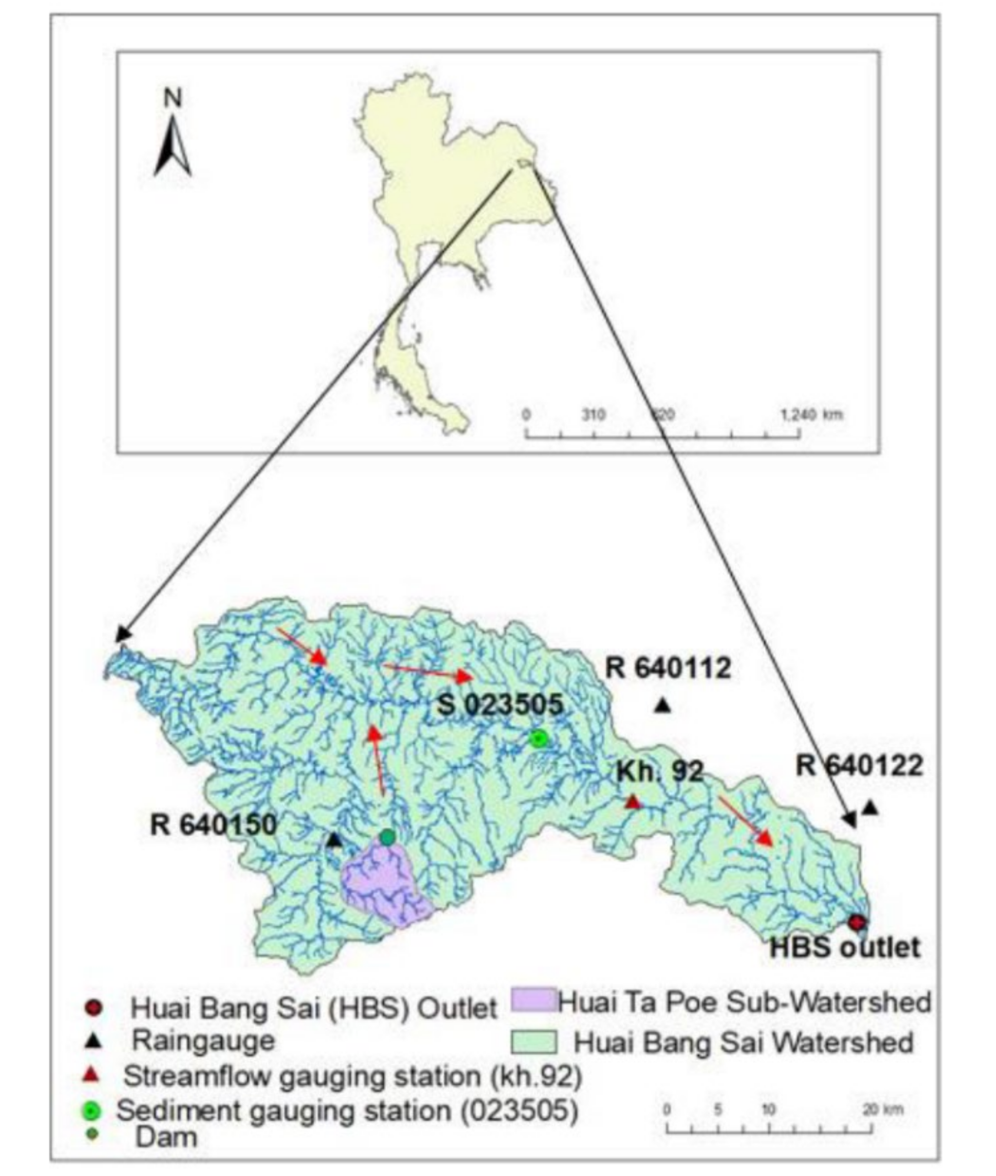
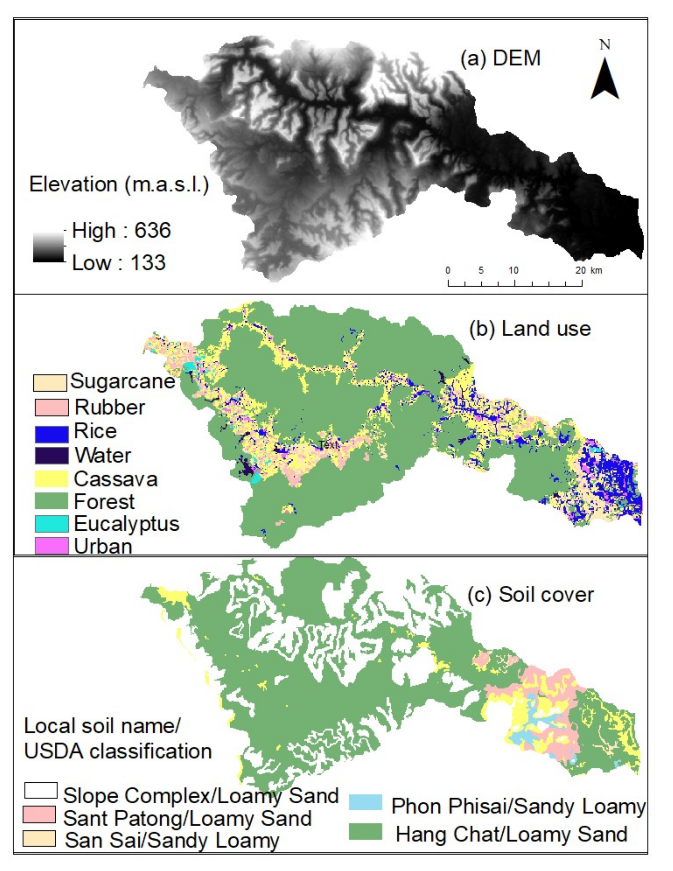
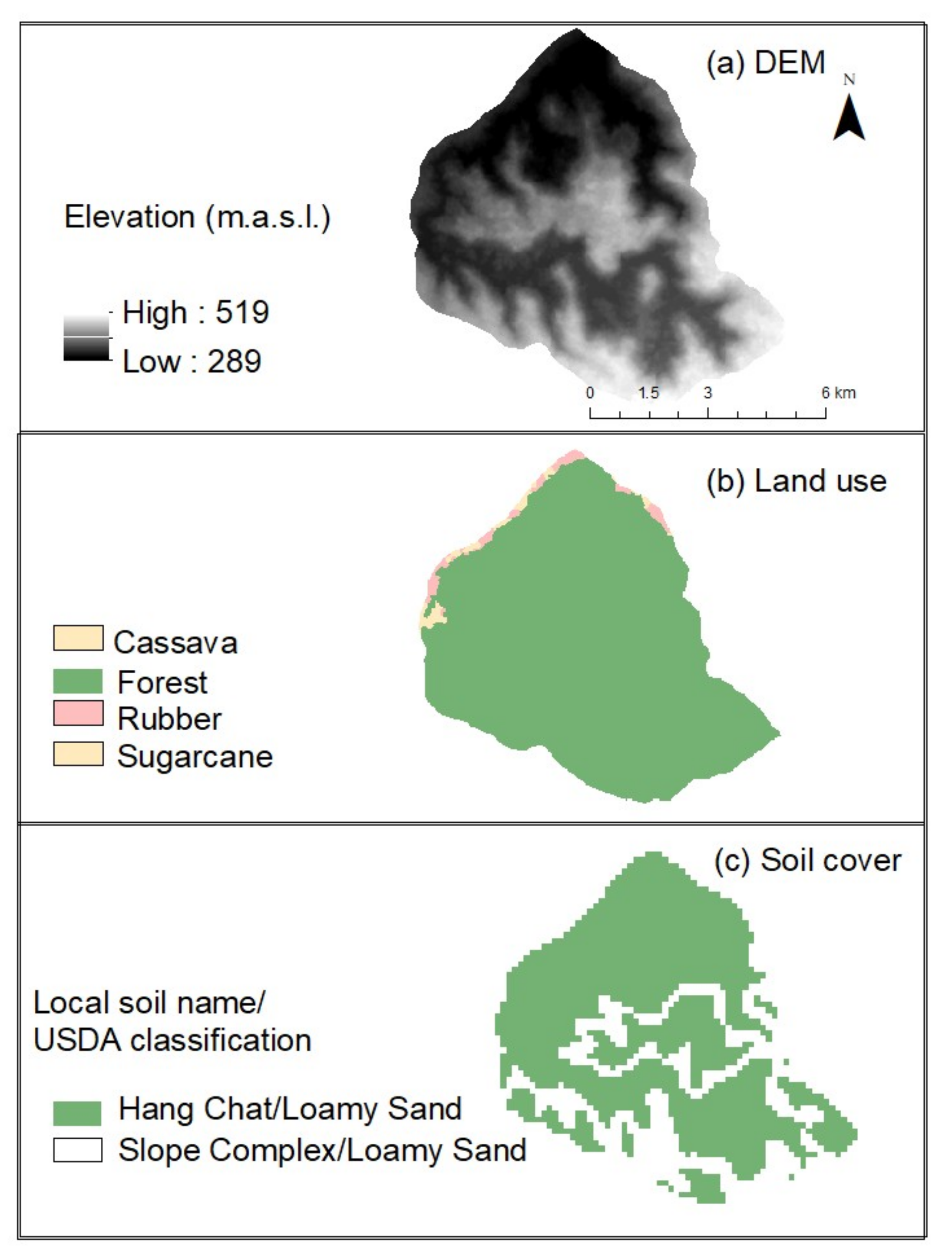
2.1. Study Area
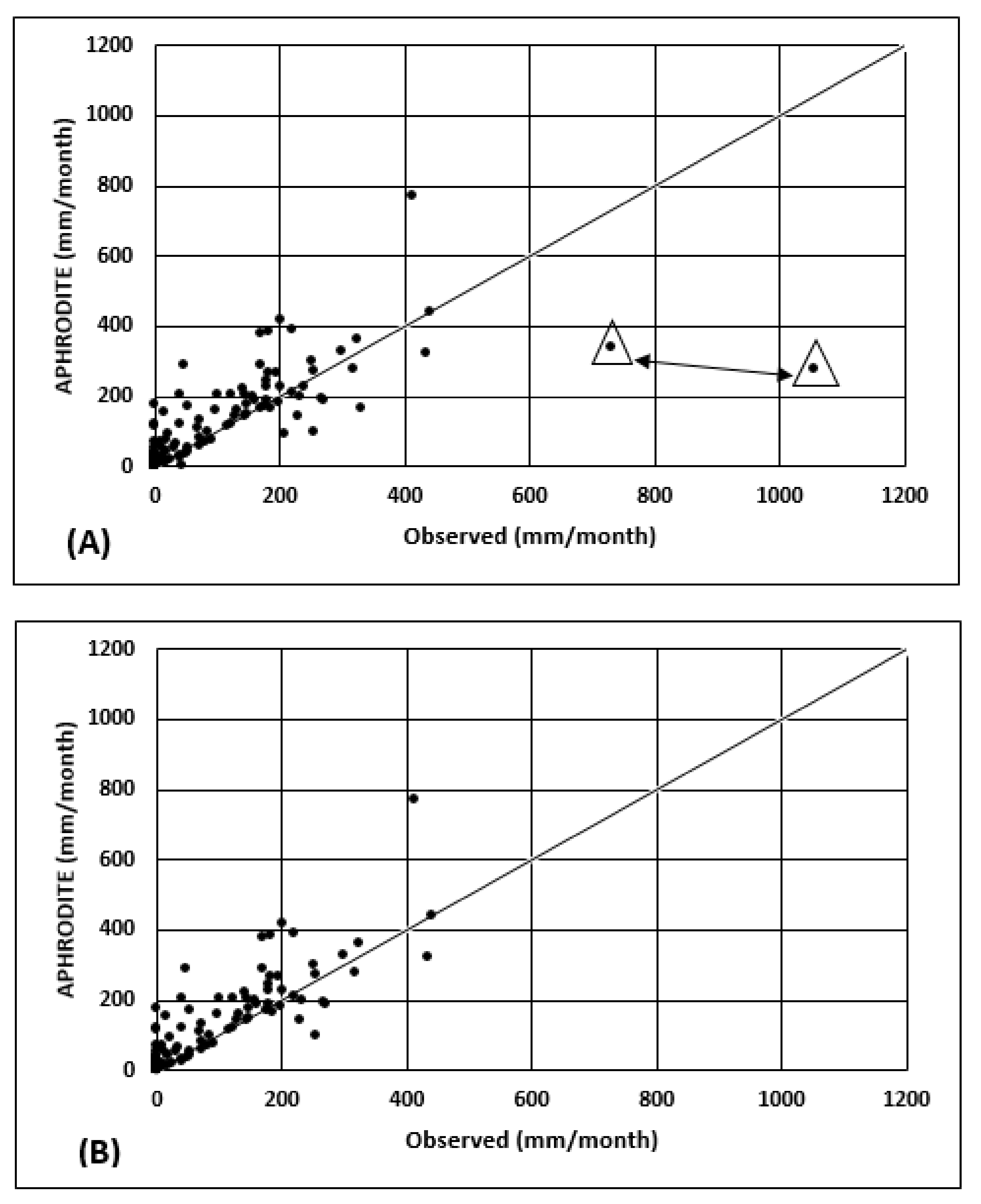
2.2. Data
2.3. SWAT Model
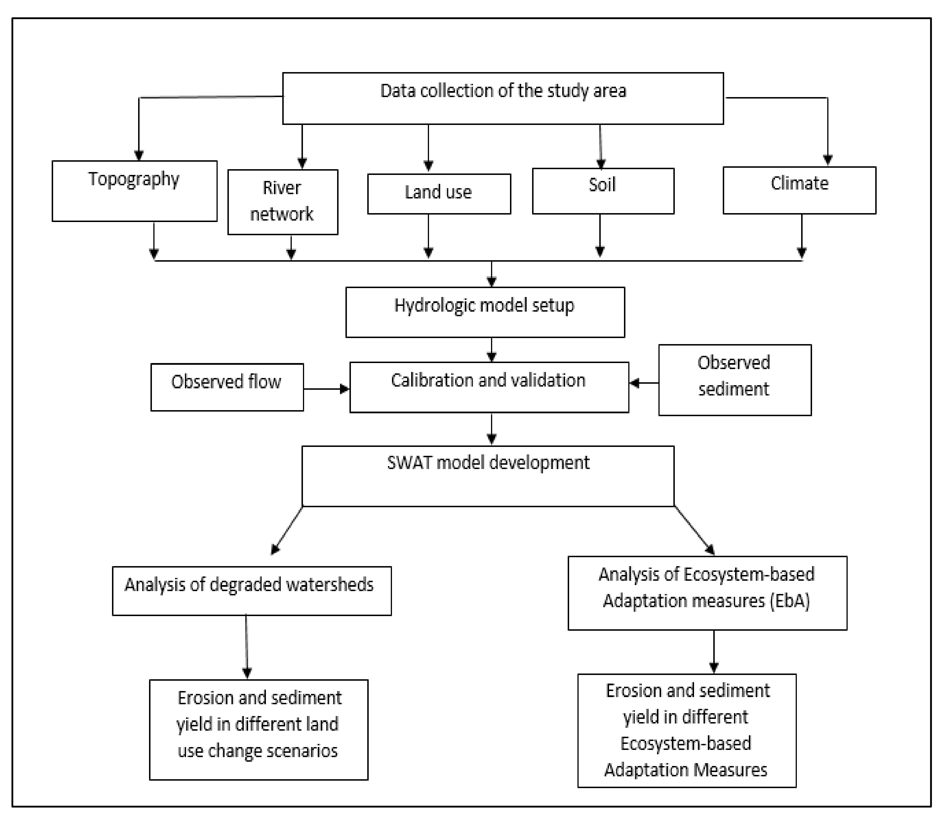
2.4. Watershed Model Development
2.5. Watershed Degradation (Land-Use Change) Scenarios
2.6. Ecosystem-Based Adaptation (EbA) Measures
3. Results and Discussion
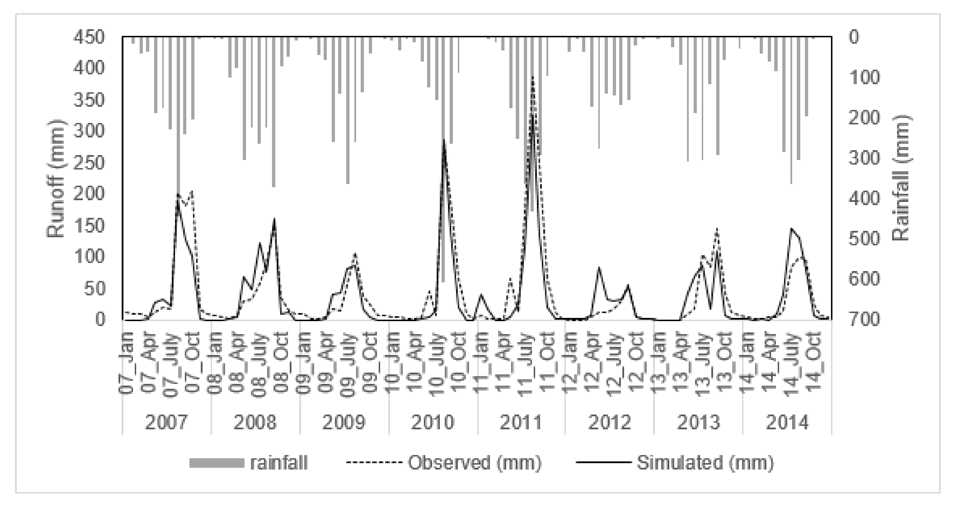
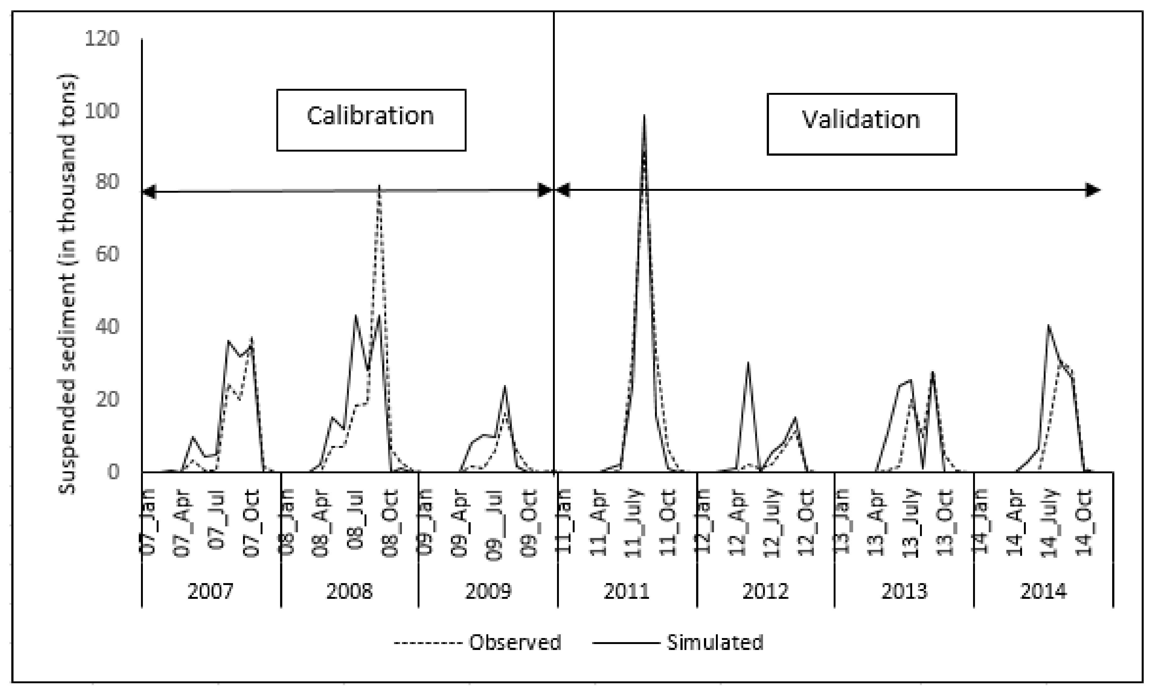
3.1. Watershed Model Calibration and Validation
3.1.1. Streamflow
3.1.2. Sediment
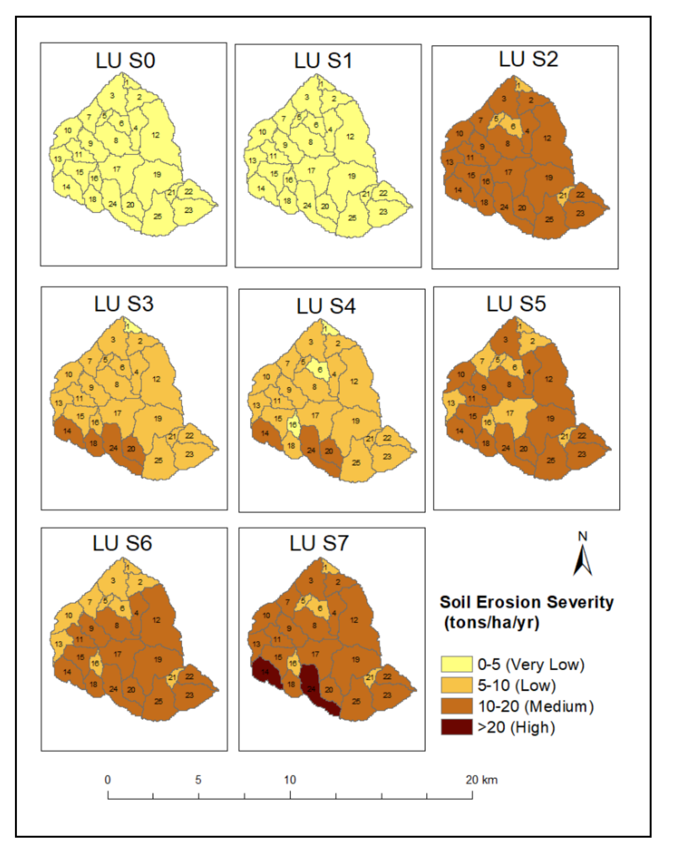
3.2. Analysis of Degraded Watersheds
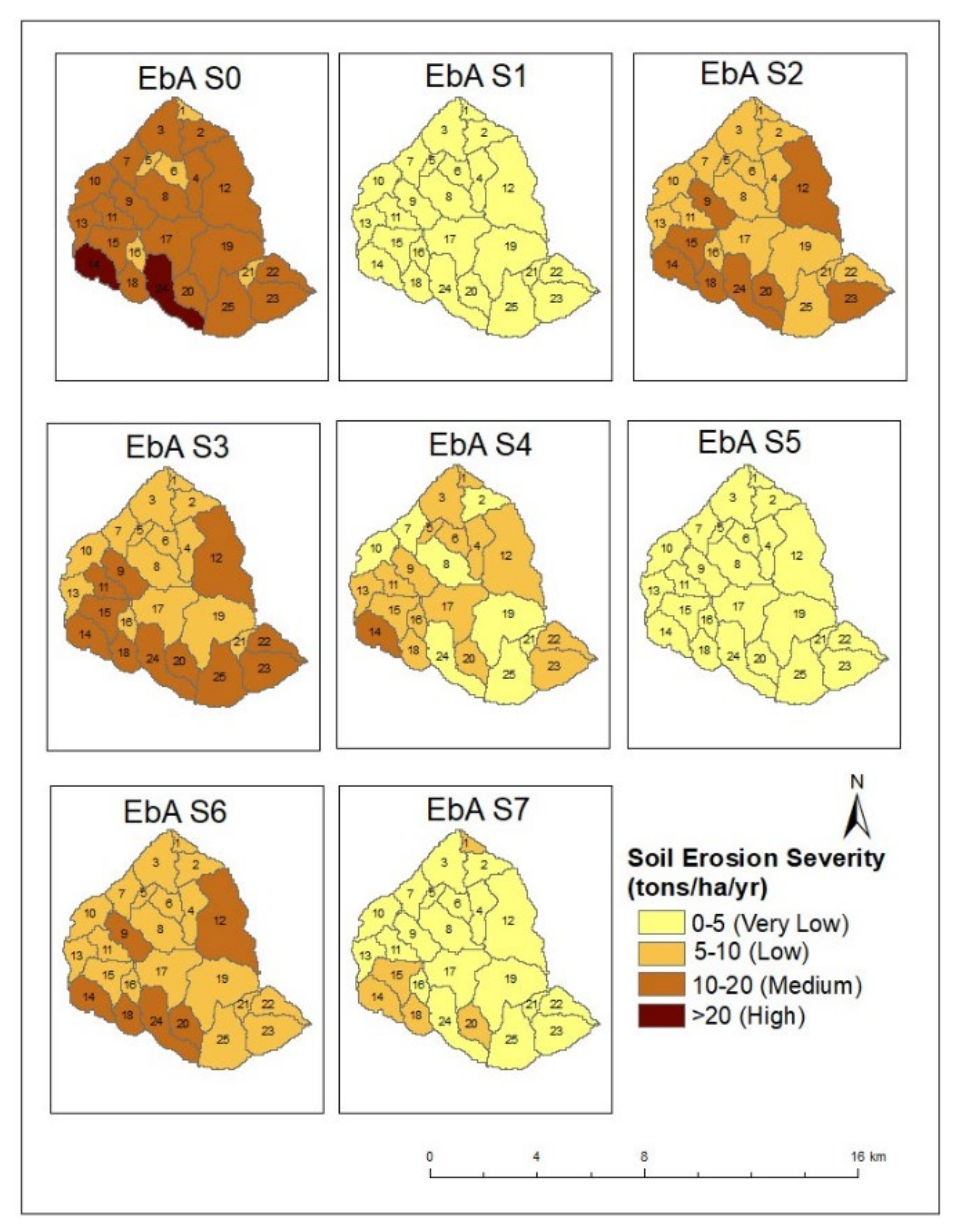
3.3. Evaluation of EbA Measures
4. Conclusions
Author Contributions
Funding
Institutional Review Board Statement
Informed Consent Statement
Data Availability Statement
Conflicts of Interest
Appendix A

| Land-Use Change Scenario | Sugarcane | Cassava | Rubber | Deciduous Forest | ||||
|---|---|---|---|---|---|---|---|---|
| km2 | % | km2 | % | km2 | % | km2 | % | |
| LU S0 | 0.12 | 0.20 | 0.42 | 0.86 | 0.64 | 1.34 | 46.9 | 97.6 |
| LU S1 | 10.6 | 22 | - | - | - | - | 37.5 | 78 |
| LU S2 | - | - | 30.8 | 64 | - | - | 17.3 | 36 |
| LU S3 | - | - | - | - | 38 | 79 | 10.1 | 21 |
| LU S4 | 11 | 23 | - | - | 27 | 56 | 10.1 | 21 |
| LU S5 | 10.6 | 22 | 20.2 | 42 | - | - | 17.3 | 36 |
| LU S6 | - | - | 21.5 | 44.6 | 16.0 | 33.3 | 10.6 | 22.1 |
| LU S7 | 11 | 23 | 20.2 | 42 | 6.7 | 14 | 10.1 | 21 |
| Land-Use Scenario | Very Low (0–5 t/ha/yr) | Low (5–10 t/ha/yr) | Medium (10–20 t/ha/yr) | High (>20 t/ha/yr) |
|---|---|---|---|---|
| LU S0 | 100% | - | - | - |
| LU S1 | 100% | - | - | - |
| LU S2 | - | 5% | 95% | - |
| LU S3 | 1% | 84% | 15% | - |
| LU S4 | 5% | 83% | 12% | - |
| LU S5 | - | 22% | 78% | - |
| LU S6 | - | 24% | 76% | - |
| LU S7 | - | 7% | 84% | 9% |
References
- Li, Z.; Deng, X.; Yin, F.; Yang, C. Analysis of Climate and Land Use Changes Impacts on Land Degradation in the North China Plain. Adv. Meteorol. 2015, 2015, 1–11. [Google Scholar] [CrossRef]
- Thanapakpawin, P.; Richey, J.; Thomas, D.; Rodda, S.; Campbell, B.; Logsdon, M. Effects of land use change on hydrologic regime of the Mae Chaem river basin, Northwest Thailand. J. Hydrol. 2006, 334, 215–230. [Google Scholar] [CrossRef]
- Ayoubi, S.; Sadeghi, N.; Afshar, F.A.; Abdi, M.R.; Zeraatpisheh, M.; Rodrido-Comino, J. Impacts of oak deforestation and rainfed cultivation on soil redistribution processes across hillslopes using 137Cs techniques. For. Ecosyst. 2021, 8, 1–14. [Google Scholar] [CrossRef]
- Foley, J.A.; DeFries, R.; Asner, G.P.; Barford, C.; Bonan, G.; Carpenter, S.R.; Chapin, F.S.; Coe, M.T.; Daily, G.C.; Gibbs, H.K.; et al. Global consequences of land use. Science 2005, 309, 570–574. [Google Scholar] [CrossRef] [PubMed] [Green Version]
- Gibbs, H.K.; Ruesch, A.S.; Achard, F.; Clayton, M.K.; Holmgren, P.; Ramankutty, N.; Foley, J.A. Tropical forests were the primary sources of new agricultural land in the 1980s and 1990s. Proc. Natl. Acad. Sci. USA 2010, 107, 16732–16737. [Google Scholar] [CrossRef] [PubMed] [Green Version]
- Lambin, E.F.; Gibbs, H.K.; Ferreira, L.; Grau, R.; Mayaux, P.; Meyfroidt, P.; Morton, D.C.; Rudel, T.K.; Gasparri, I.; Munger, J. Estimating the world’s potentially available cropland using a bottom-up 20. Glob. Environ. Chang. 2013, 23, 892–901. [Google Scholar] [CrossRef]
- Lugato, E.; Smith, P.; Borrelli, P.; Panagos, P.; Ballabio, C.; Orgiazzi, A.; Fernandez-Ugalde, O.; Montanarella, L.; Jones, A. Soil erosion is unlikely to drive a future carbon sink in Europe. Sci. Adv. 2018, 4, 1–8. [Google Scholar] [CrossRef] [Green Version]
- Vaezi, A.R.; Abbasi, M.; Keestra, S.; Cerda, A. Assessment of soil particle erodibility and sediment trapping using check dams in small semi-arid catchments. Catena 2017, 157, 227–240. [Google Scholar] [CrossRef] [Green Version]
- Ahmad, N.; Pandey, P. Assessment and monitoring of land degradation using geospatial technology in Bathinda district, Punjab, India. Solid Earth 2018, 9, 75–90. [Google Scholar] [CrossRef] [Green Version]
- Nickerson, C.; Ebel, R.; Borchers, A.; Carriazo, F. Major Uses of Land in the United States; EIB-89; United States Department of Agriculture, Economic Research Service: Washington, DC, USA, 2011. [Google Scholar]
- Panagos, P.; Barcelo, S.; Bourauni, F.; Bosco, C.; Dewitte, O.; Gardi, C.; Erhad, M.; Hervas De Deigo, F.; Hiederer, R.; Jeffery, S.; et al. The State of Soil in Europe—A Contribution of the JRC to the European Environment Agency’s Environment State and Outlook Report—SOER 2010; Office for Official Publications of the European Communities, Publications Office of the European Union: Luxembourg, 2012. [Google Scholar]
- Panagos, P.; Borrelli, P.; Poesen, J.; Ballabio, C.; Lugato, E.; Meusberger, K.; Montanarella, L.; Alewell, C. The new assessment of soil loss by water erosion in Europe. Environ. Sci. Policy 2015, 54, 438–477. [Google Scholar] [CrossRef]
- Abe, S.; Wakatsuki, T. Sawah Ecotechnology—A Trigger for a Rice Green Revolution in Sub-Saharan Africa: Basic Concept and Policy Implications. Outlook Agric. 2011, 40, 221–227. [Google Scholar] [CrossRef] [Green Version]
- Ejeta, G. African green revolution needn’t be a mirage. Science 2010, 327, 831–832. [Google Scholar] [CrossRef] [PubMed] [Green Version]
- Aglanu, L.M. Watersheds and rehabilitations measures-A review. Resour. Environ. 2014, 4, 104–114. [Google Scholar]
- Kheereemangkla, Y.; Shrestha, R.; Shrestha, S.; Jourdain, D. Modeling Hydrologic Response to Land Management Scenarios for the Chi River Sub-basin Part-2, Northeast Thailand. Environ. Earth Sci. 2016, 75, 2–16. [Google Scholar] [CrossRef]
- Imai, N.; Furukawa, T.; Tsujino, R.; Kitamura, S.; Yumoto, T. Factors affecting forest area change in Southeast Asia during 1980–2010. PLoS ONE 2018, 13, e0197391. [Google Scholar] [CrossRef] [PubMed] [Green Version]
- Hafner, J.; Apichatvullop, Y.; Subhadhira, S. Northeast Thailand Upland Social Forestry Project. 2016. Human-Forest Interactions in Northeast Thailand: A Summary Report for the Ford Foundation, Thailand; Ford Foundation: Bangkok, Thailand, 1987. [Google Scholar]
- Arfanuzzaman, M.; Dahiya, B. Sustainable urbanization in Southeast Asia and beyond: Challenges of population growth, land use change, and environmental health. Growth Chang. 2019, 50, 725–744. [Google Scholar] [CrossRef]
- Wicke, B.; Sikkema, R.; Dornburg, V.; Faaij, A. Exploring land use changes and the role of palm oil production in Indonesia and Malaysia. Land Use Policy 2011, 28, 193–206. [Google Scholar] [CrossRef]
- Lim, C.L.; Prescott, G.W.; De Alban, J.D.T.; Ziegler, A.D.; Webb, E.L. Untangling the proximate causes and underlying drivers of deforestation and forest degradation in Myanmar. Conserv. Biol. 2017, 31, 1362–1372. [Google Scholar] [CrossRef] [Green Version]
- Herath, G.; Hasanov, A. Climate Change and Threats to Sustainability in South East Asia: Dynamic Modelling Approach for Malaysia. In Regional Growth and Sustainable Development in Asia; New Frontiers in Regional Science: Asian Perspectives, 7; Batabyal, A., Nijkamp, P., Eds.; Springer: Cham, Switzerland, 2017. [Google Scholar]
- Stocker, T.F.; Qin, D.; Plattner, G.-K.; Tignor, M.; Allen, S.K.; Boschung, J.; Nauels, A.; Xia, Y.; Bex, V.; Midgley, P.M. (Eds.) Climate Change 2013: The Physical Science Basis. Contribution of Working Group I to the Fifth Assessment Report of the Intergovernmental Panel on Climate Change; Cambridge University Press: Cambridge, UK; New York, NY, USA, 2013. [Google Scholar]
- Borrelli, P.; Robinson, D.A.; Panagos, P.; Lugato, E.; Yang, J.E.; Alewell, C.; Wuepper, D.; Montanarella, L.; Ballabio, C. Land use and climate change impacts on global soil erosion by water (2015–2070). Proc. Natl. Acad. Sci. USA 2020, 117, 21994–22001. [Google Scholar] [CrossRef]
- Food and Agriculture Organization. World Fertilizer Trends and Outlook to 2018; Food and Agriculture Organization: Rome, Italy, 2015. [Google Scholar]
- Lutz, W.; Butz, W.P.; Samir, K.C. World Population and Human Capital in the Twenty-First Century; IISA: Luxemborg, 2014. [Google Scholar]
- Kayama, M.; Himmapan, W. Improvement of Utilization Techniques of Forest. Resources to Promote Sustainable Forestry in Thailand; JIRCAS Working Report No.85; Japan International Research Center for Agricultural Sciences: Tsukuba, Japan, 2017. [Google Scholar]
- Leblond, J.P. Revisiting forest transition explanations: The role of “push” factors and adaptation strategies in forest expansion in northern Phetchabun, Thailand. Land Use Policy 2019, 83, 195–214. [Google Scholar] [CrossRef]
- Homdee, T.; Pongput, K.; Kanae, S. Impacts of land cover changes on hydrologic responses. A case study of Chi River Basin, Thailand. J. Jpn. Soc. Civ. Eng. Ser. B1 (Hydraul. Eng.) 2011, 67, 31–36. [Google Scholar] [CrossRef] [Green Version]
- Gathagu, J.N.; Sang, J.K.; Maina, C.W. Modelling the Impacts of Structural Conservation Measures on Sediment and water yield in Thika-Chania Catchment, Kenya. Int. Soil Water Conserv. Res. 2018, 6, 165–174. [Google Scholar] [CrossRef]
- Darghouth, S.; Ward, C.; Gambarelli, G.; Styger, C. Roux Watershed Management Approaches, Policies and Operations: Lessons for Scaling Up; Water sector board discussion paper series, Paper no. 11; World Bank: Washington, DC, USA, 2008. [Google Scholar]
- Pansak, W.; Hilger, T.H.; Dercon, G.; Kongkaew, T.; Cadisch, G. Changes in relationship between soil erosion and N loss pathways after establishing soil conservation systems in uplands of Northeast Thailand. Agric. Ecosyst. Environ. 2008, 128, 167–176. [Google Scholar] [CrossRef]
- Cohen-Shacham, E.; Walters, G.; Janzen, C.; Maginnis, S. Nature-Based Solutions to Address Global Societal Challenges; International Union of Conservation Research: Gland, Switzerland, 2016. [Google Scholar]
- Jang, S.; Ahn, S.; Kim, S. Evaluation of executable best management practices in Haean highland agricultural catchment of South Korea using SWAT. Agric. Water Manag. 2017, 180, 224–234. [Google Scholar] [CrossRef]
- Emerton, L. Valuing the Benefits, Costs and Impacts of Ecosystem-Based Adaptation Measures: A Source Book of Methods for Decision-Making; Deutsche Gesellschaft für Internationale Zusammenarbeit (GIZ) GmbH.: Bonn, Germany, 2017. [Google Scholar]
- Jha, M.K. Evaluating Hydrologic Response of an Agricultural Watershed for Watershed analysis. Water 2011, 3, 604–617. [Google Scholar] [CrossRef]
- Amatya, D.M.; Jha, M.K.; Williams, T.M.; Edwards, A.E.; Hitchcock, D.R. SWAT Model Prediction of Phosphorus Loading in South Carolina Karst Watershed with a Downstream Embayment. J. Environ. Prot. 2012, 4, 75–90. [Google Scholar] [CrossRef] [Green Version]
- Schilling, K.E.; Gassman, P.W.; Kling, C.L.; Campbell, T.; Jha, M.K.; Wolter, C.F.; Arnold, J.G. The Potential for Agricultural Land Use Change to Reduce Flood Risk in a Large Watershed. Hydrol. Process. 2014, 28, 3314–3325. [Google Scholar] [CrossRef]
- Burkart, C.S.; Jha, M.K. Site-specific Simulation of Nutrient Control Policies: Integrating Economic and Water quality effects. J. Agric. Resour. Econ. West. Agric. Resour. Organ. 2012, 37, 20–23. [Google Scholar]
- Feng, H.; Jha, M.K.; Gassman, P.W. The Allocation of Nutrient Load Reduction Across a Watershed: Assessing Delivery Coefficients as an Implementation Tool. Rev. Agric. Econ. 2009, 31, 183–204. [Google Scholar] [CrossRef]
- Ndomb, P.N.; Mtalo, F.W.; Killingtveit, A. A Guided Swat Model Application On Sediment Yield Modeling In Pangani River Basin: Lessons Learnt. J. Urban Environ. Eng. 2008, 2, 53–62. [Google Scholar] [CrossRef]
- Kling, C.L.; Panagopoulos, I.; Rabotyagov, S.; Valcu, A.; Gassman, P.W.; Campbell, T.; White, M.J.; Arnold, J.G.; Srinivasan, R.; Jha, M.K.; et al. LUMINATE: Linking agricultural land use, local water quality and Gulf of Mexico hypoxia. Eur. Rev. Agric. Econ. 2014, 41, 431–459. [Google Scholar] [CrossRef]
- Jha, M.K.; Pan, Z.; Takle, E.S.; Gu, R. Impacts of Climate Change on Streamflow in the Upper Mississippi River Basin: A Regional Climate Model Perspective. J. Geophys. Res. Atmos. 2004, 109, 1–12. [Google Scholar] [CrossRef]
- Jha, M.K.; Arnold, J.G.; Gassman, P.W.; Giorgi, F.; Gu, R. Climate Change Sensitivity Assessment on Upper Mississippi River Basin Streamflows Using SWAT. J. Am. Water Resour. Assoc. 2007, 42, 997–1015. [Google Scholar] [CrossRef]
- Jha, M.K.; Gassman, P.W.; Panagopoulos, Y. Regional Changes in Nitrogen Loadings in the Upper Mississippi River Basin Under Predicted Mid-century Climate. Reg. Environ. Chang. 2015, 15, 449–460. [Google Scholar] [CrossRef]
- Takle, E.S.; Jha, M.K.; Lu, E.; Arritt, R.W.; Gutowski, W.J. Streamflow in the Upper Mississippi River Basin as simulated by SWAT driven by 20th Century contemporary results of global climate models and NARCCAP regional climate models. Meteorologische Zeitschift 2010, 19, 341–346. [Google Scholar] [CrossRef] [Green Version]
- Lu, E.; Takle, E.S.; Jha, M.K. The Relationships Between Climatic and Hydrological Changes in the Upper Mississippi River Basin: A SWAT and Multi-GCM Study. J. Hydrometeorol. 2010, 11, 437–451. [Google Scholar] [CrossRef] [Green Version]
- Jha, M.K.; Gassman, P.W. Changes in Hydrology and Streamflow as Predicted by Modeling Experiment Forced with Climate Models. Hydrol. Process. 2014, 28, 2772–2781. [Google Scholar] [CrossRef]
- Chattopadhyay, S.; Jha, M.K. Hydrologic Response Due to Projected Climatic Variability in Haw River Watershed, North Carolina, USA. Hydrol. Sci. J. 2016, 61, 495–506. [Google Scholar] [CrossRef]
- Arnold, J.G.; Srinivasan, R.; Muttiah, R.S.; Williams, J.R. Large Area Hydrologic Modeling and Assessment: Part I. Model development. J. Am. Water Resour. Assoc. 1998, 34, 73–89. [Google Scholar] [CrossRef]
- Munoz-Carpena, R.; Parsons, J.; Gilliam, J.W. Modeling Hydrology and Sediment Transport in Vegetative Filter Strips. J. Hydrol. 1999, 214, 111–129. [Google Scholar] [CrossRef]
- Ciou, S.K.; Kuo, J.T.; Hsieh, P.H.; Yu, G.H. Optimization Model for BMP Placement in a Reservoir Watershed. J. Irrig. Drain. Eng. 2012, 138, 736–747. [Google Scholar] [CrossRef]
- Williams, C.O.; Lowrance, R.; Potter, T.; Bosch, D.D.; Strickland, T. Atrazine transport within a coastal zone in Southeastern Puerto Rico: A sensitivity analysis of an agricultural field model and riparian zone management model. Environ. Model. Assess. 2016, 21, 751–761. [Google Scholar] [CrossRef] [Green Version]
- Li, Z.; Luo, C.; Xi, Q.; Li, H.; Pan, J.; Zhou, Q.; Xiong, Z. Assessment of Ann-AGNPS Model in Simulating Runoff and Nutrients in a Typical Small Watershed in the Taihu Lake Basin, China. Catena 2015, 133, 349–361. [Google Scholar] [CrossRef]
- Chen, N.; Hong, H.; Cao, W.; Zhang, Y.; Wang, W. Assessment of Management Practices in a Small Agricultural Watershed in Southeast China. J. Environ. Sci. Health (Part A) 2006, 41, 1257–1269. [Google Scholar] [CrossRef]
- Jha, M.K.; Rabotyagov, S.; Gassman, P.W. Optimal Placement of Conservation Practices Using Genetic Algorithm with SWAT. Int. Agric. Eng. J. 2009, 18, 41–50. [Google Scholar]
- Barnhart, B.; Lu, Z.; Bostian, M.; Sinha, A.; Deb, K.; Kurkalova, L.; Jha, M.K.; Whittaker, G. Handling Practicalities in Agricultural Policy Optimization for Water Quality Improvements. In Proceedings of the Genetic and Evolutionary Computation Conference (GECCO 2017), Berlin, Germany, 15–19 July 2017. [Google Scholar]
- Liu, Y.; Yang, W.; Leon, L.; Wong, I.; McCrimmon, C.; Dove, A.; Fong, P. Hydrologic modeling and evaluation of Best Management Practice scenarios for the Grand River watershed in Southern Ontario. J. Great Lakes Res. 2016, 42, 1289–1301. [Google Scholar] [CrossRef]
- Elci, A. Evaluation of nutrient retention in vegetated filter strips using SWAT model. Water Sci. Technol. 2017, 76, 2742–2752. [Google Scholar] [CrossRef] [PubMed] [Green Version]
- Betrie, G.D.; Mohamed, Y.A.; Van Griensven, A.; Srinivasan, R. Sediment Management Modelling in the Blue Nile Basin Using SWAT Model. Hydrol. Earth Syst. Sci. 2011, 15, 807–818. [Google Scholar] [CrossRef] [Green Version]
- Briak, H.; Mrabet, R.; Moussadek, R.; Aboumaria, K. Use of a calibrated SWAT model to evaluate the effects of agricultural BMPs on sediments of the Kalaya river basin (North of Morocco). Int. Soil Water Conserv. Res. 2019, 7, 176–183. [Google Scholar] [CrossRef]
- Merriman, K.R.; Daggupati, P.; Srinivasan, R.; Hayhurst, B. Assessment of site-specific agricultural Best Management Practices in the Upper East River watershed, Wisconsin, using a field-scale SWAT model. J. Great Lakes Res. 2019, 45, 619–641. [Google Scholar] [CrossRef]
- Graiprab, P.; Pongput, K.; Tangtham, N.; Gassman, P. Hydrologic evaluation and effect of climate change on the At Samat watershed, Northeast Region, Thailand. Int. Agric. Eng. J. 2010, 19, 12–22. [Google Scholar]
- Wangpimool, W.; Pongput, K.; Sukvibool, C.; Sombatpanit, S.; Gassman, P. The Effect of Reforestation on Streamflow in Upper Nan River Basin Using Soil and Water Assessment Tool (SWAT) Model. Int. Soil Water. Conserv. Res. 2013, 1, 53–63. [Google Scholar] [CrossRef] [Green Version]
- Reungsang, P.; Kanwar, R.S.; Jha, M.K.; Gassman, P.W.; Ahmad, K.; Saleh, A. Calibration and Validation of SWAT for the Upper Maquoketa River Watershed; Working Paper 05-WP 396; Center for Agricultural and Rural Development, Iowa State University: Ames, IA, USA, 2005. [Google Scholar]
- Reungsang, P.; Kanwar, R.; Srisuk, K. Application of SWAT model in simulating stream flow for the Chi River Subbasin-2 in Northeast Thailand. Trends Res. Sci. Technol. 2010, 2, 23–28. [Google Scholar]
- Phomcha, P.; Wirojanagud, P.; Vangpaisal, T.; Thaveevouthi, T. Predicting Sediment Discharge in an Agricultural Watershed. A Case Study of the Lam Sonthi Watershd, Thailand. Sci. Asia 2011, 37, 43–50. [Google Scholar] [CrossRef]
- Pandey, A.; Bishal, K.C.; Kalura, P.; Chowdary, V.M.; Jha, C.S.; Cerdà, A. Soil Water Assessment Tool (SWAT) Modeling Approach to Prioritize Soil Conservation Management in River Basin Critical Areas Coupled With Future Climate Scenario Analysis. Air Soil Water Res. 2021, 14, 1–7. [Google Scholar] [CrossRef]
- Arunrat, N.; Kongsurakan, P.; Sereenonchai, S.; Hatano, R. Soil Organic Carbon in Sandy Paddy Fields of Northeast Thailand: A Review. Agronomy 2020, 10, 1061. [Google Scholar] [CrossRef]
- Paiboonvorachat, C.; Oyana, T.J. Land-cover changes and potential impacts on soil erosion in the Nan watershed, Thailand. Int. J. Remote Sens. 2011, 32, 6587–6609. [Google Scholar] [CrossRef]
- Lorsirirat, K.; Maita, H. Soil Erosion Problems in Northeast Thailand: A Case Study from the View of Agricultural Development in a Rural Community Near Khon Kaen in Disaster Mitigation of Debris Flows, Slope Failures and Landslide; Universal Academy Press, Inc.: Tokyo, Japan, 2006. [Google Scholar]
- Nontananandh, S.; Changnoi, B. Internet GIS, Based on USLE Modeling, for Assessment of Soil Erosion in Songkhram Watershed, Northeastern of Thailand. Kasetsart J. Nat. Sci. 2012, 46, 272–282. [Google Scholar]
- Puktlang, W.; Mongkolsawat, C.; Suwanwerakamtorn, R. The Impact of Expanding Rubber Tree Plantation on Soil Erosion in the Mekong-Sub Basin. In In Proceedings of the 34th Asian Conference on Remote Sensing 2013, ACRS, Bali, Indonesia, 20–24 October 2013. [Google Scholar]
- Lohr, H.; Sattler, K. Improved Management of Extreme Events through Ecosystem-Based Adaptation in Watersheds; Deutsche Gesellschaft für Internationale Zusammenarbeit: Hamburg, Germany, 2017. [Google Scholar]
- Yatagi, A.; Kamiguchi, K.; Arakawa, O.; Hamada, A.; Yasutomi, N.; Kitoh, A. Constructing a Long-Term Daily Gridded Precipitation Dataset for Asia Based on a Dense Network of Rain Gauges. Bull. Am. Meteorol. Soc. 2012, 93, 1401–1415. [Google Scholar] [CrossRef]
- Gassman, P.; Arnold, J.G.; Srinivasan, R.; Reyes, M. The Worldwide Use of the SWAT Model: Technological Drivers, Networking Impacts, and Simulation Trends. In Proceedings of the ASABE—21st Century Watershed Technology: Improving Water Quality and Environment, Guacimo, Costa Rica, 21–24 February 2010. [Google Scholar]
- Arnold, J.G.; Moriasi, D.N.; Gassman, P.W.; Abbaspour, K.C.; White, M.J.; Srinivasan, R.; Santhi, C.; Harmel, R.D.; Van Griensven, A.; Van Liew, M.W.; et al. SWAT: Model Use, Calibration and Validation. Trans. ASABE 2012, 55, 1491–1508. [Google Scholar] [CrossRef]
- Neitsch, S.; Arnold, J.; Kiniry, J.; Williams, J. Soil and Water Assessment Tool: Theoretical Documentation Version 2009; Texas Water Resources Institute: College Station, TX, USA, 2011. [Google Scholar]
- Bagnold, R.A. Bed load transport by natural rivers. Water Resour. Res. 1977, 13, 312. [Google Scholar] [CrossRef]
- Paiboonsak, S.; Chanket, U.; Mongkolsawat, C.; Yommaraka, B.; Wattanakit, N. Spatial Modeling for Soil Erosion Risk in Upper Chi Basin, Northeast Thailand. In Proceedings of the 26th Asian Conference on Remote Sensing, Hanoi, Vietnam, 7–11 November 2005. [Unpublished work]. [Google Scholar]
- Jha, M.; Gassman, P.W.; Arnold, J. Water Quality Modeling for the Raccoon River Watershed Using SWAT. Am. Soc. Agric. Biol. Eng. 2007, 50, 479–493. [Google Scholar]
- Abbaspour, K. SWAT-CUP User Manual, SWAT Calibration and Uncertainty Programs; EAWAG: Zurich, Switzerland, 2015. [Google Scholar]
- International Renewable Energy Agency. Renewable Energy Outlook: Thailand; International Renewable Energy Agency: Abu-Dhabi, UAE, 2017. [Google Scholar]
- Pumkaew, W. Joint Management of Biofuel Production and Food Production to Optimize Energy Return to Land Use in Thailand: A Regional Mathematical Programming Approach. Ph.D. Thesis, Clemson University, Clemson, SC, USA, December 2019. [Google Scholar]
- Fox, J.; Castella, J.C. Expansion of rubber (Hevea brasiliensis) in Mainland SoutheastAsia: What are the prospects for smallholders? J. Peasant Stud. 2013, 40, 155–170. [Google Scholar] [CrossRef]
- Rendana, M.; Rahim, S.; Lihan, T. Spatial Modeling Based Analysis of Land Suitability for Rubber Crops in Ranau District, Malaysia. Am. Eurasian J. Agric. Environ. Sci. 2014, 14, 1019–1025. [Google Scholar]
- Ahmed, G.B.; Shariff, A.R.M.; Idrees, M.O.; Balasundram, S.K.; Abdullah, A.F.B. GIS-Based Land Suitability Mapping for Rubber Cultivation in Seremban, Malaysia. Int. J. Appl. Eng. Res. 2017, 12, 9420–9433. [Google Scholar]
- Samarappuli, L.; Wijesuriya, W.; Dissanayake, D.; Karunaratne, S.; Herath, H. Land Suitability for Sustainable Rubber Cultivation in Moneragala District. J. Environ. Prof. 2014, 3, 48–61. [Google Scholar] [CrossRef] [Green Version]
- Jamil, M.; Ahmed, R.; Sajjad, H. Land suitability assessment for sugarcane cultivation in Bijnor district, India using geographic information system and fuzzy analytical hierarchy process. GeoJournal 2018, 83, 595–611. [Google Scholar] [CrossRef]
- Laxmikantam, M. Technology in Sugarcane Growing, 2nd ed.; Oxford and IBH Publication: Culcutta, India, 1983. [Google Scholar]
- Kakade, J.R. Sugarcane Cultivation; Metropolitan Book Company PVT. Ltd.: New Delhi, India, 1985. [Google Scholar]
- Purnamasari, R.; Ahamed, T.; Noguchi, R. Land Suitability Assessment for Cassava Production in Indonesia Using GIS, Remote Sensing and Multi-criteria Analysis. Asia Pac. J. Reg. Sci. 2018, 3, 1–32. [Google Scholar] [CrossRef]
- Grismer, M.; O’Geen, A.; Lewis, D. Vegetative Filter Strips for Non-Point Source Pollution Control in Agriculture; Publication 8195; Division of Agriculture and Natural Resources, University of California: California, CA, USA, 2006. [Google Scholar]
- Department of Environmental Water Quality. Storm Water Best Management Practices Catalog; Department of Environmental Quality (DEQ): Boise, ID, USA, 2005. [Google Scholar]
- United States Department of Agriculture, Manual on Conservation Practice Standard; United States Department of Agriculture: Washington, DC, USA, 2016.
- Arabi, M.; Frankenberger, J.R.; Engel, B.A.; Arnold, J.G. Representation of Agricultural Conservation Practices with SWAT. Hydrol. Process. 2008, 22, 3042–3055. [Google Scholar] [CrossRef]
- Mwangi, J.K.; Shisanya, C.A.; Gathenya, J.M.; Namirembe, S.; Moriasi, D.N. A Modeling Approach to Evaluate the Impact of Conservation Practices on Water and Sediment Yield in Sasumua Watershed, Kenya. J. Soil Water Conserv. 2015, 70, 75–90. [Google Scholar] [CrossRef] [Green Version]
- Fiener, P.; Auerswald, K. Seasonal Variation of Grassed Waterway Effectiveness in Reducing Runoff and Sediment Delivery from Agricultural Watersheds in Temperate Europe. Soil Tillage Res. 2006, 87, 48–58. [Google Scholar] [CrossRef]
- Babel, M.S.; Shrestha, B.; Perret, S. Hydrogical impact of biofuel production: A case study of the Khlong Phlo Watershed in Thailand. Agric. Water Manag. 2011, 101, 8–26. [Google Scholar] [CrossRef]
- Sudjarit, W.; Pukngam, S.; Tangtham, N. Application of SWAT model for assessing effect of main functions of watershed ecosystem in Headwater, Thailand. Proc. Int. Acad. Ecol. Environ. Sci. 2015, 5, 57–69. [Google Scholar]
- Moriasi, D.N.; Arnold, J.G.; Van Liew, M.W.; Bingner, R.L.; Harmel, R.D.; Veith, T.L. Model Evaluation Guidelines for Systematic Quantification of Accuracy in Watershed Simulations. Trans. ASABE 2007, 50, 885–900. [Google Scholar] [CrossRef]
- Gull, S.; Ma, A.; Dar, A. Prediction of streamflow and sediment yield of Lolab Watershed using SWAT model. Hydrol. Curr. Res. 2017, 8, 1–9. [Google Scholar] [CrossRef] [Green Version]
- Yesuf, H.; Assen, M.; Alamirew, T.; Melesse, A. Modeling of sediment yield in Maybar gauged watershed using SWAT, Northeast Ethiopia. Catena 2015, 127, 191–205. [Google Scholar] [CrossRef]
- Moench, M. Soil Erosion Under a Succession Agro Forestry Sequence: A case study from Idukki District, Kerala, India. Agrofor. Syst. 1991, 15, 31–50. [Google Scholar] [CrossRef]
- Vongkasem, W.; Klakhaeng, K.; Hemvijit, S.; Tongglum, A.; Katong, S.; Suparhan, D.; Howeler, R.H. Reducing soil erosion in cassava production systems in Thailand: A farmer participatory approach. In Cassava’s Potential in Asia in the 21st Century: Present Situation and Future Research and Development Needs, Proceedings of the Sixth Regional Workshop, Ho Chi Minh City, Vietnam, 21–25 February 2000; Howeler Reinhardt, H., Tan Swee, L., Eds.; Cassava Office for Asia: Bangkok, Thailand.
- Putthacharoen, S. Nutrient removal by crops and nutrient loss by erosion in cassava in comparison with that of other crops. Master’s Thesis, Kasetsart University, Bangkok, Thailand, 1992. [Google Scholar]
- Putthacharoen, S.; Howeler, R.H.; Jantawat, S.; Vichukit, V. Nutrient uptake and soil erosion losses in cassava and six other crops in a Psamment in Eastern Thailand. Field Crop. Res. 1998, 57, 113–126. [Google Scholar]
- Da Silva, V.S.G.; De Oliveira, M.W.; Oliveira, T.B.A.; Mantovanelli, B.C.; Da Silva, A.C.; Soares, A.N.R.; Clemente, P.R.A. Leaf area of sugarcane varieties and their correlation with biomass productivity in three cycles. Afr. J. Agric. Res. 2017, 12, 459–466. [Google Scholar]
- Cotter, M.; Asch, F.; Hilger, T.; Rajaona, A.; Schappert, A.; Stuerz, S.; Yang, X. Measuring leaf area index in rubber plantations−A challenge. Ecol. Indic. 2017, 82, 357–366. [Google Scholar] [CrossRef]
- Lahai, M.T.; Ekanayake, I.J.; Koroma, J.P.C. Influence of canopy structure on yield of cassava cultivars at various toposequences of an inland valley agro ecosystem. J. Agric. Biotechnol. Sustain. Dev. 2013, 5, 36–47. [Google Scholar] [CrossRef] [Green Version]
- Chanthorn, W.; Ratanapongsai, Y.; Brockelman, W.Y.; Allen, M.A.; Favier, C.; Dubois, M.A. Viewing tropical forest succession as a three-dimensional dynamical system. Theor. Ecol. 2015, 9, 163–172. [Google Scholar] [CrossRef]
- Sharma, A. Integrating Terrain and Vegetation Indices for Identifying Potential Soil Erosion Risk Area. Geo Spat. Inf. Sci. 2010, 13, 201–209. [Google Scholar] [CrossRef]
- Marden, M. Effectiveness of reforestation in erosion mitigation and implications for future sediment yields, East Coast catchments, New Zealand: A review. New Zealand Geogr. 2012, 68, 24–35. [Google Scholar] [CrossRef]
- Gassman, P.W.; Osei, E.; Saleh, A.; Rodecap, J.; Norvell, S.; Williams, J. Alternative Practices for Sediment and Nutrient Loss Control on Livestock Farms in Northeast Iowa. Agric. Ecosyst. Environ. 2006, 117, 135–144. [Google Scholar] [CrossRef]
- Schmidt, E.; Zernadim, B. Expanding Sustainable Land Management in Ethiopia: Scenarios for Improved Agricultural Water Management in the Blue Nile. Agric. Water Manag. 2015, 158, 166–178. [Google Scholar] [CrossRef]
- Arabi, M.; Govindaraju, R.S.; Hantush, M.M.; Engel, B.A. Role of Watershed Subdivision on Modeling the Effectiveness of Best Management Practices. J. Am. Water Resour. Assoc. 2006, 42, 513–528. [Google Scholar] [CrossRef]
- Taffarello, D.; Calijuri, M.D.C.; Viani, R.A.G.; Marengo, J.A.; Mendiondo, E.M. Hydrological services in the Atlantic Forest, Brazil: An ecosystem-based adaptation using eco-hydrological monitoring. Clim. Serv. 2017, 8, 1–16. [Google Scholar] [CrossRef]
- United Nations Environmental Programme. Green Infrastructure. Guide for Water Management: Ecosystem-based Management Approaches for Water-Related Infrastructure projects; United Nations Environmental Program: Nairobi, Kenya, 2014. [Google Scholar]
- Wischmeier, W.H.; Smith, D.D. Predicting Rainfall Erosion Losses: A Guide to Conservation Planning; US Department of Agriculture, Agricultural Handbook No.537; US Government Printing Office: Washington, DC, USA, 1978.
- United States Department of Agriculture. Manual on Natural Resources Conservation Practice Standard: Terraces-Code 600; Natural resources Conservation Services: Washington, DC, USA, 2009. [Google Scholar]


| Data Type and Station | Temporal Resolution | Spatial Resolution | Period | Source |
|---|---|---|---|---|
| Temporal data | ||||
| Temperature Sakon Nakhon Nakhon Phanom Nakon Phanom Agromet | Daily | Point data | 2004–2014 | TMD |
| Rainfall 640150 640112 640122 | Daily | Point data | 2004–2014 | RID |
| Gridded rainfall | Daily | 0.5 × 0.5° | 1985–2014 | APHRODITE |
| Streamflow kh. 92 Drainage area: 1118 km2 | Daily | Point data | 2007–2014 | RID |
| Suspended Sediment 023505 Drainage area: 928 km2 | Daily | Point data | 2007–2014 | DWR |
| Spatial data | ||||
| DEM | - | 30 × 30 m | - | USGS |
| Soil cover | - | 1 × 1 km | - | LDD |
| Land use | - | 500 × 500 m | - | LDD |
| Land Use Type | ||
|---|---|---|
| Deciduous forest | 0.01 | 1 |
| Cassava | 0.20 | 1 |
| Rubber | 0.44 | 0.35 |
| Sugarcane | 0.01 | 1 |
| Rangeland | 0.03 | 1 |
| Rice | 0.03 | 0.10 |
| Water | 0 | 0 |
| Urban areas | 0 | 0.001 |
| Eucalyptus | 0.01 | 1 |
| Scenario | Description |
|---|---|
| LU S0 | Baseline: Existing land use |
| LU S1 | Sugarcane on land areas with slope less than 5% |
| LU S2 | Cassava on land areas with slope between 0% and 15% |
| LU S3 | Rubber on land areas with slope between 0% and 20% |
| LU S4 | Sugarcane on land areas with slope from 0% to 5%, Rubber on land areas with slope from 5% to 20% |
| LU S5 | Sugarcane on land areas with slope from 0% to 5%, Cassava on land areas with slope from 5% to 15% |
| LU S6 | Cassava on land areas with slope from 0% to 10%, Rubber on land areas with slope from 10% to 20% |
| LU S7 | Sugarcane on land areas with slope from 0% to 5%,Cassava on land areas with slope from 5% to 15%, Rubber on land areas with slope from 15% to 20% |
| Scenario | Description |
|---|---|
| EbA S0 | baseline scenario (same as LU S7) |
| EbA S1 | reforestation of all land areas |
| EbA S2 | filter strips to land areas with slope less than 10% |
| EbA S3 | contouring to land areas with slope less than 10% |
| EbA S4 | terracing to land areas with slope more than 10% |
| EbA S5 | reforestation + filter strips + grassed waterways |
| EbA S6 | contouring + filter strips + grassed waterways |
| EbA S7 | terracing + filter strips + grassed waterways |
| EbA Measure | SWAT Parameter(s) | Application Criteria | Reference |
|---|---|---|---|
| Reforestation | Land-use code | Any land use | [60] |
| Filter strips | FILTER_W = 10 m | Slopes less than 10% | [60,93,94] |
| Contouring | Reduce CN by 3 units and adjust USLE_P based on slope | Agricultural lands of slopes less than 10% | [30,95] |
| Terracing | Reduce CN by 6 units and adjust USLE_P based on slope | Agricultural lands of slopes higher than 10% | [96,97] |
| Grassed waterways | Adjust Manning’s roughness coefficient (n), channel erodibility factor (CH_EROD) and channel cover factor (CH_COV) | Main channel and tributary reaches | [96,98] |
| Rank | Parameter | Description | Initial Values | Fitted Value |
|---|---|---|---|---|
| 1 | CN | SCS-CN Deciduous forest Cassava Sugarcane Rice Rubber Rangeland Water Urban | 73–92 77 85 85 81 77 79 92 90 | 73 83 83 81 77 79 92 90 |
| 2 | ESCO | Soil evaporation compensation factor | 0.95 | 0.70–0.95 |
| 3 | SOL_AWC | Available soil water capacity Hang Chat/Loamy sand Slope Complex/Loamy sand Miscellaneous soil San Sai/Sandy loamy Phon Phisai/Sandy loamy San Patong/Loamy sand | 0.14 0.14 0.14 0.10 0.10 0.10 | 0.10 0.10 0.10 0.13 0.14 0.15 |
| 4 | ALPHA_BF | Base-flow alpha factor | 0.048 | 0.99 |
| 5 | GW_DELAY | Ground water delay | 31 | 2 |
| 6 | GW_REVAP | Groundwater “revap” coefficient | 0.02 | 0.19 |
| Scenario | Description | Simulated Sediment Yield in HRUs (103 tons/ha/year | Simulated Sediment Outflux at Outlet (103 tons/ha/year) | Calculated Sediment Deposition (103 tons/ha/year) (Erosion-Outflux) |
|---|---|---|---|---|
| (1) | (2) | (3) = (1) − (2) | ||
| LU S0 | 97.52% forest, 1.34% rubber, 0.86% cassava, 0.28% sugarcane | 2.3 | 0.5 | 1.8 |
| LU S1 | 78% forest, 22% sugarcane | 2.1 | 0.6 | 1.5 |
| LU S2 | 36% forest, 64% cassava | 12.7 | 0.7 | 12 |
| LU S3 | 21% forest 79% rubber | 7.7 | 0.7 | 7 |
| LU S4 | 21% forest, 56% rubber, 23% sugarcane | 7.3 | 0.7 | 6.6 |
| LU S5 | 36% forest, 42% cassava, 22% sugarcane | 11.7 | 0.8 | 10.9 |
| LU S6 | 22% forest, 33% rubber, 45% cassava | 11.6 | 0.8 | 10.8 |
| LU S7 | 21% forest, 14% rubber, 42% cassava, 23% sugarcane | 13.5 | 0.8 | 12.7 |
| Scenario | Description | Simulated Sediment Yield of HRUs (103 tons/ha/year) | Simulated Sediment Outflux at the Outlet (103 tons/ha/year) | Calculated Sediment Deposit (103 tons/ha/year) |
|---|---|---|---|---|
| EbA S0 | Baseline Scenario (Degraded watershed LU S7) | 13.5 | 0.8 | 12.7 |
| EbA S1 | Reforestation (R) (Forest to all lands) | 2.2 | 0.5 | 1.7 |
| EbA S2 | Filter Strips (FS) (All lands with slope < 10%) | 9.8 | 0.7 | 9.0 |
| EbA S3 | Contouring (C) (All lands with slope < 10%) | 10.4 | 0.8 | 9.3 |
| EbA S4 | Terracing (T) (All lands with slope > 10%) | 5.4 | 0.8 | 4.6 |
| EbA S5 | R+FS+GW | 1.6 | 0.1 | 1.5 |
| EbA S6 | C+FS+GW | 8.3 | 0.1 | 8.2 |
| EbA S7 | T+FS+GW | 5.2 | 0.1 | 5.1 |
| Scenario | Precipitation (mm) | Surface Runoff (mm) | Lateral Flow (mm) | Evapotranspiration (mm) | Groundwater Flow (mm) |
|---|---|---|---|---|---|
| EbA S0 | 1218 | 221 | 283 | 492 | 222 |
| EbA S1 | 1218 | 133 | 277 | 636 | 172 |
| EbA S2 | 1218 | 221 | 282 | 494 | 221 |
| EbA S3 | 1218 | 201 | 284 | 495 | 238 |
| EbA S4 | 1218 | 205 | 288 | 495 | 230 |
| EbA S5 | 1218 | 133 | 277 | 636 | 172 |
| EbA S6 | 1218 | 201 | 284 | 495 | 238 |
| EbA S7 | 1218 | 205 | 288 | 495 | 238 |
Publisher’s Note: MDPI stays neutral with regard to jurisdictional claims in published maps and institutional affiliations. |
© 2021 by the authors. Licensee MDPI, Basel, Switzerland. This article is an open access article distributed under the terms and conditions of the Creative Commons Attribution (CC BY) license (https://creativecommons.org/licenses/by/4.0/).
Share and Cite
Babel, M.S.; Gunathilake, M.B.; Jha, M.K. Evaluation of Ecosystem-Based Adaptation Measures for Sediment Yield in a Tropical Watershed in Thailand. Water 2021, 13, 2767. https://doi.org/10.3390/w13192767
Babel MS, Gunathilake MB, Jha MK. Evaluation of Ecosystem-Based Adaptation Measures for Sediment Yield in a Tropical Watershed in Thailand. Water. 2021; 13(19):2767. https://doi.org/10.3390/w13192767
Chicago/Turabian StyleBabel, Mukand S., Miyuru B. Gunathilake, and Manoj K. Jha. 2021. "Evaluation of Ecosystem-Based Adaptation Measures for Sediment Yield in a Tropical Watershed in Thailand" Water 13, no. 19: 2767. https://doi.org/10.3390/w13192767
APA StyleBabel, M. S., Gunathilake, M. B., & Jha, M. K. (2021). Evaluation of Ecosystem-Based Adaptation Measures for Sediment Yield in a Tropical Watershed in Thailand. Water, 13(19), 2767. https://doi.org/10.3390/w13192767