
Identifying Spatial Driving Factors of Energy and Water Consumption in the Context of Urban Transformation


1
Department of Land Resources, Chinese Culture University, Taipei 11114, Taiwan
2
Department of Environmental Engineering, National Cheng Kung University, Tainan 701401, Taiwan
3
Graduate Institute of Environmental Engineering, National Taiwan University, Taipei 10617, Taiwan
4
Department of Civil and Construction Engineering, National Taiwan University of Science and Technology, Taipei 10607, Taiwan
*
Authors to whom correspondence should be addressed.
Sustainability 2021, 13(19), 10503; https://doi.org/10.3390/su131910503
Submission received: 27 July 2021
/
Revised: 1 September 2021
/
Accepted: 17 September 2021
/
Published: 22 September 2021
(This article belongs to the Special Issue Construction Project and Management in Smart Cities)
Abstract
:Urban energy and water consumption varies substantially across spatial and temporal scales, which can be attributed to changes of socio-economic variables, especially for a city undergoing urban transformation. Understanding these variations in variables related to resource consumptions would be beneficial to regional resource utilization planning and policy implementation. A geographically weighted regression method with modified procedures was used to explore and visualize the relationships between socio-economic factors and spatial non-stationarity of urban resource consumption to enhance the reliability of predicted results, taking Taichung city with 29 districts as an example. The results indicate that there is a strong positive correlation between socio-economic context and domestic resource consumption, but that there are relatively weak correlations for industrial and agricultural resource consumption. In 2015, domestic water and energy consumption was driven by the number of enterprises followed by population and average income level (depending on the target districts and sectors). Domestic resource consumption is projected to increase by approximately 84% between 2015 and 2050. Again, the number of enterprises outperforms other factors to be the dominant variable responsible for the increase in resource consumption. Spatial regression analysis of non-stationarity resource consumption and its associated variables offers useful information that is helpful for targeting hotspots of dominant resource consumers and intervention measures.
1. Introduction
By 2050, worldwide energy and water consumption is forecasted to increase by 80% and 55% (compared with the level in the year 2000), respectively [1]. The stress on resource consumption comes from increasing demand, which is driven by the growing population as well as by shifts in anthropogenic processes [2,3,4,5,6]. Urbanization is considered one of the most vital anthropogenic alterations [7], and urban patterns are often used to dictate the concentration and distribution of such alterations. Urban patterns can be defined by a city’s area, aggregation, spatial metrics [8], and coupling with anthropogenic activities, which, in turn, influence regional resource consumption through a complex mechanism [9,10,11]. Given that the altering pattern and pace of different anthropogenic activities are identified to be distinct from one another [12], then incorporate with the shifting urban pattern, resource consumption should be evaluated in a spatially and temporally focused manner to deliver a full picture.
Contemporary studies largely draw on how socio-economic variables, which can be expressed in terms of anthropogenic activity, spatial pattern, meso-economic structure, or combined effects on behavior, affect the flow of resource consumption and production [13,14,15]. These variables may include ones with socio-demographic characteristics (e.g., income level, GDP, population, household size, density) or may include built environment attributes (e.g., urban zoning, housing unit, dwelling age, floor area) [11,15,16,17,18,19,20]. Various social-economic contexts, such as socio-demographic and the built-environment, shape the specific spatial cluster attributes for a given region (township or city) and form different resource consumption patterns [16,21]. For example, variables of building types and layout, consumption behavior, and human lifestyle have been evaluated to identify spatial characteristics in recent years [22,23]. Thus, the complex spatial and temporal resource consumption facing urban transitions can be analyzed with a large quantity of spatial data of socio-economic variables [24,25]. Additionally, the consumption intensities of resource usage are dissimilar in various enterprises and in human activities under different sectors [15], and as such, they should be evaluated separately. The relationship between sectoral social-economic contexts and spatially distributed resource consumption is less investigated, and the correlations are expected to be more intense for a region undergoing urban transformation.
Various analytical models can be used to analyze the flow of energy and water consumption. Conventional input–output analysis (IOA) and life cycle assessment (LCA) are static models that are unable to capture urban spatial processes [17,26]. Regional or city-scale analysis is developed by IOA and material flow assessment (MFA) with approximations (e.g., by downscaling national flows based on population share, or share in GDP), and the assumptions of consumption intensity are often borrowed at the national level. IOA, LCA, and MFA frequently emphasize illustrated disaggregated and intersectoral resource flows, yet the spatial drivers and underlying causes of such flows are less discussed or ignored. However, spatially aggregated models are made possible with these static models coupling with intersectional resource flows and spatial data sets [27] or through simulation [28]. Nevertheless, data availability and quality, assumptions, or spatial averaging for these models may lead to different results with estimated uncertainty, as the interactions among the constituting elements are not spatially and temporally stationary [11,29]. In contrast, the analytical approach of spatial econometrics has been used to better understand the overall context and to evaluate resource consumption by incorporating socio-economic variables in a spatial-temporal manner [20,26,30]. In this study, a large quantity and detailed spatial open-source data available from the Taiwanese government are used to overcome the listed difficulties for truthful simulation.
Spatial econometric models are devised to indicate the spatial dynamics of resource consumption as a comprehensive representation of urban physical and social processes by highlighting the autocorrelation (spatial dependency), heterogeneity (spatial non-stationarity), and weighting (spatial correction) of explanatory variables. Geographically weighted regression (GWR) and ordinary least-squares (OLS) are the most commonly applied models. OLS is a stationary regression analysis, whereas GWR extends the function by adding a geographical location parameter and accounts for spatial heterogeneity through calibration [31,32,33]. Until now, GWR analysis has been extensively used in the fields of urban planning [34,35,36], environmental science [37,38,39], ecosystem [40,41,42] as well as sociology [43]. In this study, GWR with modified procedures is applied to illustrate the non-stationary nature of resource consumption in spatial structures and to outline the spatial effect of its driving variables.
For a city that undergoes major urban transformation such as massive urban renewal or municipality merger, identification of the temporal-spatial changes of socio-economic variables becomes crucial in estimating resource consumption. Additionally, the illustration of the spatial dynamics of resource consumption over a timespan is essential in order to formulate resource utilization planning to enhance resource efficiency in metropolises. This study extends current GWR approaches by considering the non-stationary spatial and temporal variation of socio-economic factors to predict water and energy consumption at township-level (second level in geographical classification) through a series of procedures. Figures of a consolidated city-county (the unified administrative body of Taichung city is used as the case study) were extracted to explore dramatic changes in socio-economic variables. To diminish the bias of long-term changes and variance in non-linear regression analysis, local indicators of spatial association (LISA) was applied to identify local clusters and to screen a better bandwidth, which is needed in GWR analysis [32,38,44,45]. Multicollinearity was removed with OLS. The above procedures are used to improve prediction accuracy of GWR.
A GWR analysis was then used to assess the spatial effects of the selected variables in a benchmark year and further to predict the resource consumption trends based on the spatial coefficient of these variables. Moreover, socio-economic variables and resource consumption are grouped into domestic, industrial, and agricultural sectors in order to analyze sectoral consumption in terms of spatial distribution and to understand how the variations in variables contribute to sectoral consumption. The findings would be of great benefit for policymaker to develop new policies or to improve the effectiveness of existing programs regarding urban activities and resource planning.
The four objectives of the current study are (a) to evaluate the spatial-temporal characteristics of socio-economic variables and to develop cluster maps for a city undergoing mass urban transformation; (b) to analyze the coefficients of water and energy consumption of the driving variables at township-level; (c) to compare the predicted results with actual data for validation; and (d) to forecast the changes in domestic water and energy consumption to provide insight for policymaking.
2. Materials and Methods
2.1. The Study Site
Taichung City consists of 29 townships and was used as the study site. Former Taichung City and Taichung County were merged to form a larger Taichung City in 2010, and it is now the second largest metropolitan area in Taiwan. A total of 70% of the precision machinery, machine tools, and parts manufacturers in Taiwan have manufacturing facilities in Taichung. Production from the local industrial clusters comprises 64.1% of the local GDP, and 35.9% of total outputs come from the service sector, with insignificant agricultural and mining activities. The total production output has increased 21.9% from 2011 to 2016, indicating that Taichung City underwent urban transformation after 2010.
The energy and water consumption datasets as well as social and economic data were taken from the Taiwan Power Company (TPC), the Water Resources Agency (WRA), and the Ministry of the Interior (MOI), respectively. Data for the consumed energy and water were available for 625 villages at village-level (third level in geographical classification) with 1020 datasets from 2015 to 2017, and socio-economic variables were released at township-level (second level).
To understand the spatial effects of socio-economic variables on resource consumption, this study first analyzes the changes of three main variables from 2011 to 2015 (two variables were excluded with missing data), and the geostatistical patterns of five socio-economic variable are identified at township-level for 2015, as summarized in Supplementary Table S1. The limitation of the available open-source data based on geographical classification [46] and the geographic changes of resource consumption is that more than 30 datasets need to be used to generate cluster maps by means of LISA analysis. The energy and water consumption at village-level is available for the year 2015 and afterwards. The benchmark year of 2015 was selected, as it represents the earliest available village-level figures. However, data regarding socio-economic variables are available at township-level for 29 towns and were excluded from LISA analysis, as the results are only reliable if the input feature class contains at least 30 features.
2.2. Study Framework and Methodology
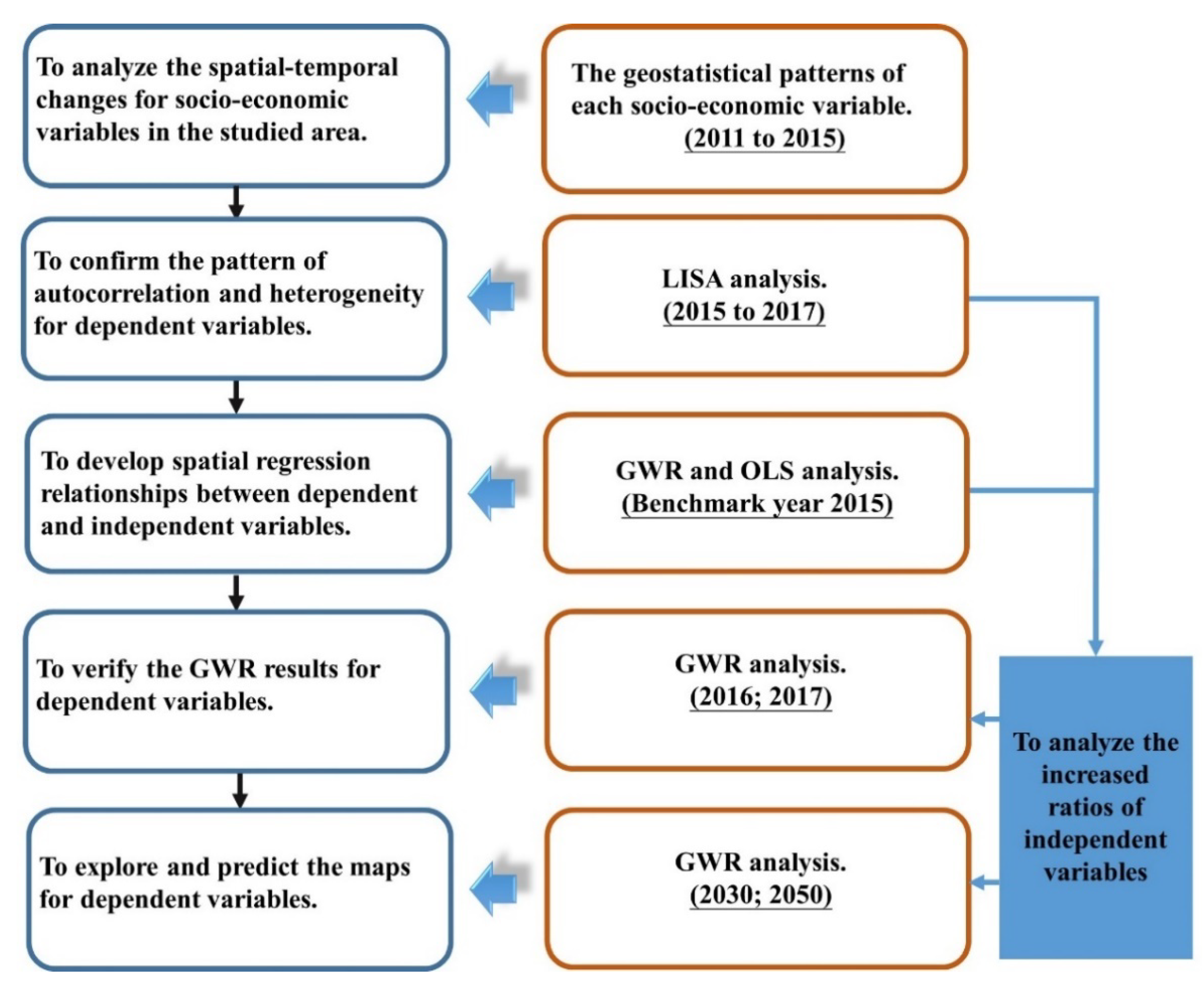
This study develops a comprehensive framework to analyze the spatial-temporal changes of regional water and energy consumption with respect to influencing factors in urban transformation, as shown in Figure 1. First, the spatial-temporal changes of the socio-economic variables for Taichung City from 2011 to 2015 were outlined to demonstrate non-stationary spatial urban transformation. To improve the estimation accuracy, the spatial cluster characteristics and the impacts of multicollinearity are required to be identified. Cluster characteristic changes of water and energy consumption at township-level from 2015 to 2017 were presented in terms of local spatial autocorrelation and heterogeneity with LISA. Additionally, applicable bandwidth was specified in the process. These are used to provide a preliminary assessment of the non-stationarity characteristics of the dependent and independent GWR variables.
Then, spatial varying energy and water consumption derived from the identified socio-economic variables were evaluated with OLS analysis and spatial regression analysis (GWR) in the benchmark year 2015. In addition, the GWR analysis results were further refined by prescreening the variance inflation factor (VIF) during the OLS analysis (also in the third step). The estimated performance of GWR was then evaluated by comparing the estimated figures with actual data from 2016 and 2017. Finally, resource consumption forecasting for the domestic sector for the years 2030 and 2050 was provided to offer useful information in decisions for public policy.
2.3. Spatial Autocorrelation and Heterogeneity
The cluster characteristics are emphasized with the use of Moran’s I and LISA to prescreen the spatial autocorrelation effects [32,36,39,43,45,47,48]. LISA is modified from Moran’s I to indicate the cluster for each location [49], and was included to provide the local spatial autocorrelation. Ii values from the LISA index are used to convert Z-score and local G-statistic to reveal the statistical significance and cluster trends. Here, the 90, 95, or 99 percent confidence levels were used. Additionally, the values with Z > 2.58 indicate a positive autocorrelation in the observations at the confidence coefficient of 99%. When Z is zero, it indicates spatial randomness.
The LISA formulas are shown as follows:
where is an attribute (energy or water consumption) for feature i; is the average value of all of the attribute values in the study area; wij is the spatial weight between feature i and j; S is the variance of ; Z(Ii) is the expected value of LISA; Ii for feature i; Gi* measures the high/low clustering for the attribute values (such as Z, Ii, or ) in the study site.
When Ii is positive, it shows similar values to a variable are found in its neighboring locations. Positive Ii determines the locations of statistically significant clusters, known as hotspots (HH or LL cluster). A negative value exists when dissimilar values in neighboring districts are reported, indicating HL or LH cluster. Then, a cluster map of four zones can be labeled based on the Z-score and the p-value of LISA, namely high–high (HH), low–high (LH), low–low (LL), and high–low (HL).
2.4. Spatial Regression Analysis
GWR is a local form of linear regression incorporating spatial non-stationarity in regression analysis [31]. The ability to visually represent the varying strength of spatial relationship between the dependent and independent variables is one benefit of GWR. In this study, GWR was used to analyze the spatial relationships between energy and water consumption and driving factors in urban transformation. The proposed approach is also beneficial for predicting hotspots for regional resource consumption by characterizing the spatial-temporal changes of the socio-economic context at township-level. The important outcomes from GWR analysis are derived from the individual regression output: every spatial dataset has its regression equation with an R2 value (R2 and adjusted R2), the predicted dependent variable, coefficient, intercept for each independent variable, residual value, and condition number. The R2 value represents the variance for a dependent variable, and the adjusted R2 value presents the better fitting results by checking Akaike information criterion (AIC). The predicted value (fitted y) is estimated by GWR; and the residual values are obtained by subtracting the fitted y values from the observed y values. The formula is as follows:
where yj represents the dependent variable; uj and vj are the coordinates for location j; β0 (uj, vj) represents the intercept for location j; and βi (uj, vj) is the local estimated coefficient for the independent variable xij; εj presents the random spatial error coefficient.
GWR coefficients are used to disclose the strong or weak correlations between the independent variables and the dependent variables, and there is a concern for possible multicollinearity [50]. Local collinearity may lead to unreliable coefficient estimates and should be treated with caution [32,50,51]. A condition number larger than 30 indicates that GWR estimation may be unreliable due to the presence of multicollinearity. Also, GWR is sensitive to kernel bandwidth, and the optimal bandwidth can be chosen by measuring the minimized AIC in GWR [32,38,40,52] or through LISA. Multicollinearity can be quantified with the help of VIF in OLS prescreening, as it may cause misleading results for regression coefficients and standard errors. Most of the independent variables with VIF > 7.5 are then excluded in GWR analysis.
3. Results and Discussion
In Taichung City, water and energy consumption datasets are available at village-level, and most of the socio-economic variables are only available at township-level. The study subdivides these variables into three classified sectors of 29 districts (township-level) for LISA, GWR, and OLS. The benchmark year of 2015 is used as the benchmark year to estimate performance valuation and predication.
3.1. Spatial-Temporal Characteristics of Energy and Water Consumption
Based on previous papers, resources consumption is influenced by socio-economic variables, both spatially and temporally. There are three main socio-economic variables that have been selected to outline the magnitude of urban transformation in terms of relative ratios from 2011 to 2015 since Taichung City was merged in 2010. Other variables with missing data from open-source information such as building attributes were excluded from the analysis. Taichung City experienced obvious spatial variations after being merged, as exhibited in Figure 2 and Supplementary Table S2. Red, orange, and yellow-colored regions indicate the townships with significant changes. The variations are found to be noticeable when considering household income (Figure 2b) and the number of commercial and industrial facilities (Figure 2c), while the population remains modest. The spatial patterns at each township state the spatial non-stationarity of these socio-economic variables for Taichung City during the evaluated period.
The geostatistic results of five socio-economic variables (along with building attributes) are summarized in Supplementary Table S1 for 29 townships to reveal the spatial characteristics. Different geostatistic types are identified, population is reported with lognormal distribution pattern, and the number of enterprises is presented with a geometric distribution pattern. These divergent geostatistic patterns of the variables largely affect spatial characteristics, such as autocorrelation and heterogeneity, for a given region.
The energy and water consumption determined with 1020 datasets for 625 villages were used in LISA analysis to reveal the spatial distribution for the years 2015, 2016, and 2017. As the map patterns of 2016 are similar to those of 2015, they are excluded in the following section. Figure 3 reveals noticeable spatial changes for energy consumption, while the clustering effects are less obvious in terms of water consumption. Areas colored in red and dark blue represent HH and LL clusters, which correspond to significant clusters of high and low values, respectively. Areas shown in orange and light blue indicate HL and LH clusters, respectively. In addition, areas with no significant changes are uncolored and are excluded to diminish the spatial error term. The results indicate that energy and water consumption is varied spatially and non-stationarily over time. For example, the HH clusters for energy consumption in 2017 have expanded extensively compared to in 2015, especially in the southern area of Taichung City.
Spatial variations of socio-economic variables and the clustering of resource consumption rates are considered to provide spatial-temporal description for the variables. HH clusters of energy and water consumption are situated (Figure 3a,c) for Xitun District, which is also the region with the highest average household income, suggesting that the level of resource consumption may be affected by household income. Additionally, other regions with HH clusters for energy consumption in 2017, such as Taiping, Wufeng, Wuri, and Dali District, are observed with non-stationary shifts in serval socio-economic variables, particularly in the number of enterprises. These findings are consistent with previous studies that showed energy usage is positively correlated with population and income level [16,53] and that building attributes [54,55], especially for built-up areas per unit, significantly affects resource consumption. However, the results are not able to conclude to what extent each variable contributes to the fluctuating resource consumption or if any spatial lag or time lag are experienced. Here, the non-stationary characteristics of spatial variation that potentially affect socio-economic variables and resource consumption for 29 townships are outlined.
3.2. Spatial Regression Analysis between Resource Consumption and Socio-Economic Variables
GWR was employed to investigate the relationship between resource consumption and socio-economic variables in order to identify the main driving force for energy and water consumption patterns for the benchmark year 2015. Seven socio-economic variables were selected based on previous studies, including the number of enterprises, average household incomes, population, household units, and building attributes (floor area and various building structure). A OLS analysis screening was conducted to reduce multicollinearity and bias prior to GWR analysis. Five out of seven independent variables were selected with low multicollinearity (VIF < 7.5 or with significant coefficients) for GWR analysis, as shown in Table 1.
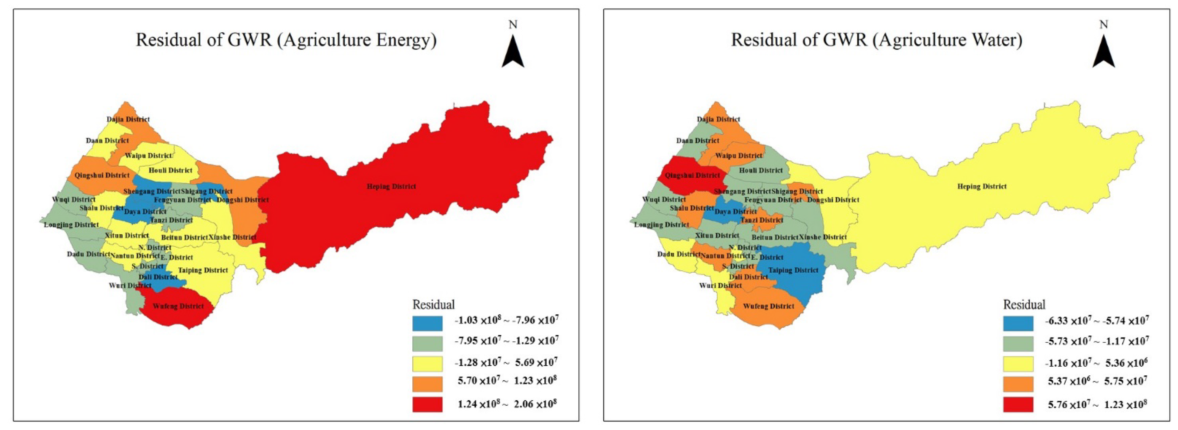
Table 2 and Table 3 summarize the average energy and water consumption coefficients as determined with GWR analysis. By comparing AIC and local R2 from OLS and GWR analysis, GWR is confirmed to have better predictive results than OLS, which can be reflected by higher adjusted R2 values, lower AIC figures and lower residual values. The local R2 values are relatively high for domestic energy and water consumption. Similarly, a higher spatial error term (ε) for GWR means a higher heterogeneity of the dependent and independent variables (higher residual value), indicating a larger gap of the fit for the GWR prediction outcome with regard to the actual data. In that sense, the resource consumption of the industrial and agricultural sectors was found to have relatively weaker correlations with socio-economic variables than those of the domestic sector. The overestimated zones with higher residual values are displayed as orange and red regions in Figure 4 and Figure 5. Overall, the residual magnitude in industrial energy consumption can be confirmed to be one thousand times larger than that of water consumption. The number of overestimated zones and residual values for the agricultural sector outnumber those of the industrial sector, particularly in the northern parts of Taichung City. Hence, downscaling resource consumption for the industrial and agricultural sectors and detailed data sets are essential to reduce spatial errors (ε) in the future.
The GWR results indicate that domestic resource consumption is positively driven by the number of enterprises, average income, population, and steel concrete structured buildings (SC). Much larger coefficient values are found for domestic energy consumption than they are for domestic water consumption for these four variables, indicating a stronger relationship between socio-economic context and domestic energy consumption.
The results reveal that the number of enterprises, population, and SC are positively correlated with both energy and water consumption, while average income and light steel-structured building (LS) are negatively correlated. This outcome is consistent with the current industry development trend that the light industry (commonly facilitated with LS) consumes less resources compared to other manufacturing activities. Additionally, the negative income phenomenon indirectly causes the changes in terms of human behavior and types of work [56].
The spatial distributions of the socio-economic variables and domestic resource consumption at township-level in 2015 are presented in Figure 6. The analysis of industrial and agricultural resource consumption has been excluded, as the correlations with socio-economic variables are relatively weak. The regions with higher coefficients are indicated in red, as those with lower coefficients are shown in green. The number of enterprises and average household income are positively correlated with resource consumption in the eastern (Heping District) and southern regions (Taiping, Wufeng, Dali, and Xinshe District) of Taichung City. A stronger correlation for the number of enterprises is observed, as the quantity of red zones representing the number of enterprises outperforms the regions representing average income. The more diversified outcomes are found in the population variable and SC for different townships. Greater population growth is reported in the eastern regions, which show lower relatedness to energy and water consumption. In contrast, weak population and SC growth are observed in Dajia, Daan, Qingshui, Wuqi, and Longjing District, but these two variables are revealed to be significantly correlated to resource consumption.
3.3. Estimate Performance of GWR Analysis
As the local R2 values estimated in the industrial and agricultural sectors in 2015 are too low to be reliable, this study focuses on comparing the GWR estimations to the actual 2016 and 2017 data to validate the estimated performance for domestic energy and water consumption. The results are shown in Table 4 and Figure 7.
The ratios in Table 4 are calculated with the prediction value as the numerator and actual data as the denominator for 29 townships. Ratios with a value larger than one indicate that these are overestimated predictions. In general, the water consumption prediction results are close to the actual data, except for Daan and Heping District, meaning that the estimated correlation coefficients between socio-economic variables and water consumption are confirmed to be well-grounded.
Conversely, most energy prediction figures are overestimated in 2016 and 2017. The differences between the predicted and actual data can be partially clarified by the energy-saving strategies implemented by the Taiwanese government in recent years [57]. These downscaling energy-saving behaviors may be difficult to capture and present in GWR analysis. Hence, in-depth variable selection and the variation evaluation of individual socio-economic variables collected over time may be required to reduce the estimating error for the overestimated energy consumption. For example, policy implementation and other macroeconomic variables may lead to behavior changes or even energy substitution [58].
Nevertheless, GWR is still a useful tool for exploring the spatial regression among various socio-economic influencing variables. The inclusion of quantified data sets characterizing resource usage behavior from different social groups is suggested in order to modify the spatial regression formula in GWR analysis in the future.
3.4. GWR Prediction of Domestic Energy and Water Consumption in 2030 and 2050
Predictions of socio-economic variables at township-level in 2030 and 2050 are estimated based on the actual data from 2011 to 2015 to forecast the future domestic energy and water consumption with GWR analysis. The domestic energy and water consumption of 29 townships demonstrate similar divergence patterns to one another. As the identical socio-economic variables are applied in both consumption projections, the expected trends and relative ratios of these two consumptions in 29 townships should be close to one another with slight variance. In that case, the conversion of domestic water and energy resource consumption into one index may be considered as a simplified estimation. Once water consumption is projected based on the reliable method and data sets, the energy consumption can be easily estimated with the defined index and vice versa. The projected results are summarized in Table 5.
If past trends of socio-economic variables continue, the overall resource consumption is forecasted to increase 1.13 times in 2030 and 1.84 times in 2050 compared to the 2015 level. The forecasted resource consumption for each township is different in order to provide a sound and representative outcome. The highest growth rate goes to N. District, which has 2.40 and 15.62 relative ratios, while the relative ratios for Heping District in both 2030 and 2050 have remained unchanged.
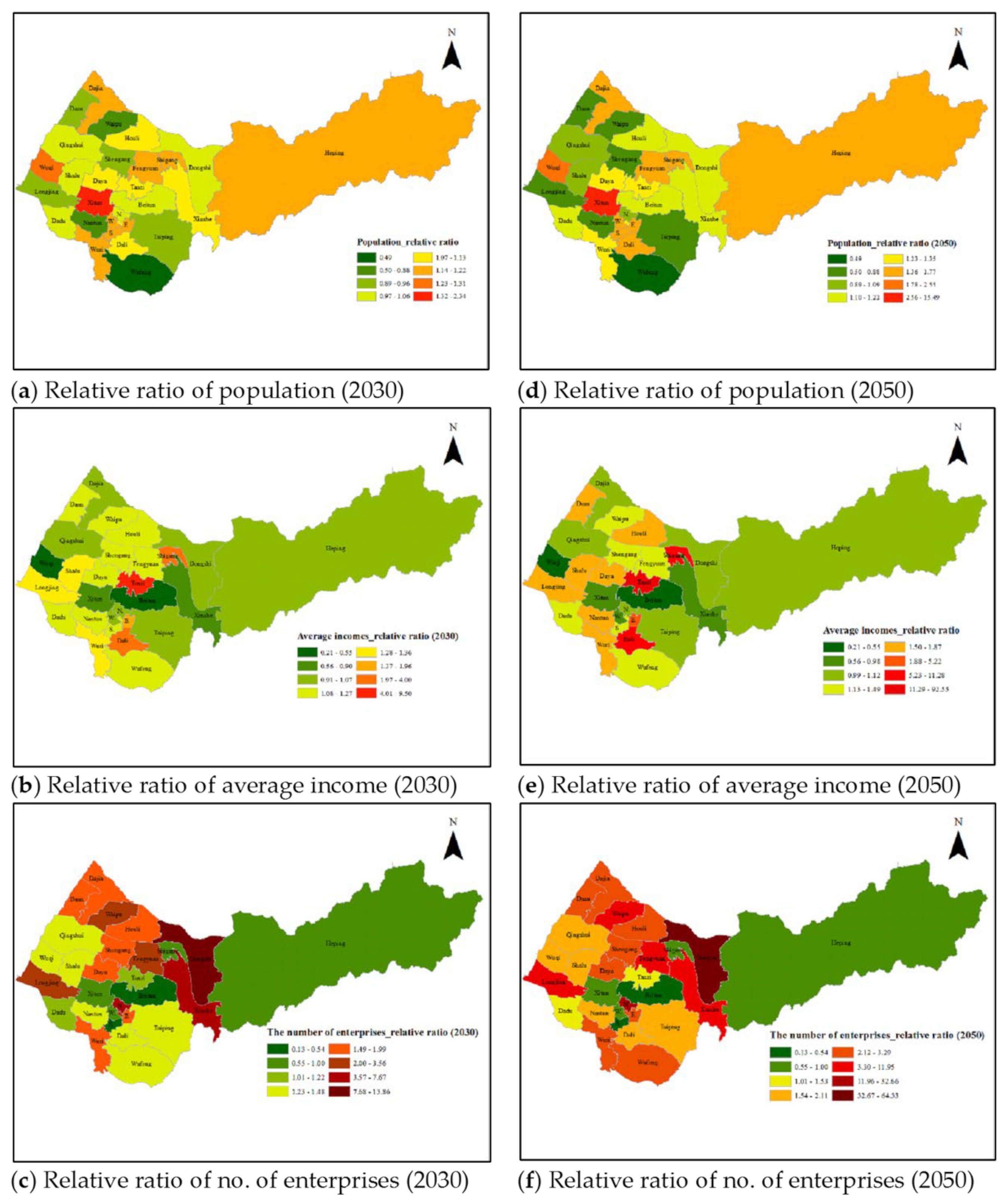
As a whole, the influence of the number of enterprises outperforms other variables in terms of how they affect domestic resource consumption greatly, with higher GWR coefficients and higher relative ratios, as revealed in Dongshi, N., and Waipu District (Figure 8). On the other hand, slight increase in the relative ratios of resource consumption in 2030 and 2050 are reported in Xitun, Dali, and Tanzi District, with strong increase in projected population and average income.
The projected results for the resource consumption and socio-economic variables of the 29 townships can be used as the evidence in regional policymaking. Hotspot indication allows the local and central governments to regulate or construct appropriate infrastructure or/and adaptive consumption strategies as the regions evolve overtime. Take N. District as an example, it is projected to have higher domestic resource consumption demands along with significant coefficients for socio-economic variables. The local council should use the projected demand against the current infrastructure capacity to identify the capacity gap or to implement resource-efficient strategies.
4. Conclusions
For a city that undergoes major urban transformation, identification of the temporal-spatial changes of the socio-economic variables becomes crucial in estimating resource consumption. This study presents a series of evaluation procedures to identify spatially and temporally varying socio-economic factors and then to estimate and predict the spatial non-stationarity effects of urban resource consumption. GWR analysis with modified procedures was used as both an exploratory and predictive tool to describe the spatial heterogeneity of association between resource consumption and five socio-economic variables for Taichung city. OLS was applied to select variables without the presence of multicollinearity, and LISA was used to reveal local clusters and to provide the optimal bandwidth for GWR. These procedures were used to achieve the minimum amount of errors and to improve the R2 value. GWR showed higher predictive power when compared to conventional linear models such as OLS with the assumption of homogeneity. The prediction performance was validated by comparing the estimated and actual data in 2016 and 2017. The predictive power of GWR was confirmed to be reliable, especially for water consumption.
The results further the understanding of energy and water consumption in the context of urban transformation as well as yield insight into resource utilization planning and sustainable policy implementation. In general, a strong correlation between number of enterprises and resource consumption was revealed, followed by population and average income level (depending on the target sectors). The regions of HH clusters were often the hotspots that experience rapid increases in the number of commercial and industrial enterprises. Noticeable sectoral differences were observed in terms of energy consumption. Positive correlations were reported between all socio-economic variables and domestic resource consumption, while both positive and negative correlations were reported for the industrial, and agricultural sectors. In sum, resource consumption of the industrial and agriculture sectors was found to have relatively weaker correlations with socio-economic variables than those of the domestic sector, indicating that the commonly used socio-economic drivers were appropriate in predicting domestic resource consumption but may not be relevant in evaluating industrial and agricultural resource consumption. A possible explanation is that industrial and agricultural consumption behaviors are more diversified depending on business activities, building structure, and characteristics. The selected socio-economic variables might not be able to reflect the usage patterns. Moreover, it is suggested that downscaling human energy-saving behaviors be included to modify the results for future research. The uncertainty of influential effects of individuals on resource consumption should also be considered, such as population. The overestimation of energy consumption derived from population growth (compared with other variables) can be partially explained by changing human behaviors over time. For example, users may be more aware of resource conservation and mitigation. Finally, the effect of spatial lag and time lag issues on the variables in terms resource consumption was unable to be located and identified in this study. Incorporation of lag effect is recommended for future research in identifying precise temporal variability of resource consumption.
As for the predication outcome, the changing pattern and coefficient of socio-economic variables are crucial in the projected resource consumption levels. The overall resource consumption is projected to increase 1.84 times in 2050 compared to the 2015 levels. The N. District was reported to have the highest relative ratio of 14.62, which is mainly due to the significant increase in the number of enterprises over time.
Consequently, through the different trends of socio-economic conditions and the spatial influence for each independent variable with the GWR results, this study predicts the hotspots for regional resource consumption based on the changes characterizing the socio-economic patterns of a city undergoing urban transformation. The conversion of domestic energy and water resource consumption into one index should be considered to simplify the estimation process and to provide a useful message for future research.
Supplementary Materials
The following are available online at https://www.mdpi.com/article/10.3390/su131910503/s1, Table S1: Statistical summary of five socio-economic variables of 29 townships for 2015, Table S2: Descriptive Statistics of socio-economic variables of 29 townships from 2011 to 2015.
Author Contributions
Conceptualization, I.-C.C. and H.-W.M.; methodology, I.-C.C.; software, I.-C.C.; validation, I.-C.C.; formal analysis, I.-C.C.; investigation, K.-L.C.; resources, C.C.W.H.; data curation, K.-L.C.; writing—original draft preparation, I.-C.C. and K.-L.C.; writing—review and editing, I.-C.C. and C.C.W.H.; visualization, I.-C.C.; supervision, H.-W.M.; project administration, C.C.W.H.; funding acquisition, I.-C.C. and C.C.W.H. All authors have read and agreed to the published version of the manuscript.
Funding
This research was funded by MOST 109-2410-H-034-026.
Institutional Review Board Statement
Not applicable.
Informed Consent Statement
Not applicable.
Data Availability Statement
Publicly available datasets were analyzed in this study. The data can be found here: Economic and social variables were taken from https://segis.moi.gov.tw/STAT/Web/Platform/QueryInterface/STAT_QueryInterface.aspx?Type=0 (accessed on 16 September 2021) Building attributes were taken from https://govstat.taichung.gov.tw/DgbasWeb/index.aspx (accessed on 16 September 2021); and https://statis.moi.gov.tw/micst/stmain.jsp?sys=100 (accessed on 16 September 2021) Energy consumptions were taken from https://egis.moea.gov.tw/opendata/ (accessed on 16 September 2021) Water consumptions were taken from https://wuss.wra.gov.tw/annuals.aspx (accessed on 16 September 2021).
Conflicts of Interest
The authors declare no conflict of interest.
References
- IRENA. Renewable Energy in the Water, Energy & Food Nexus; International Renewable Energy Agency: Abu Dhabi, United Arab Emirates, 2015. [Google Scholar]
- Huang, S.; Chen, C. Urbanization and socioeconomic metabolism in Taipei: An emergy synthesis. J. Ind. Ecol. 2009, 13, 75–93. [Google Scholar] [CrossRef]
- González, A.; Donnelly, A.; Jones, M.; Chrysoulakis, N.; Lopes, M. A decision-support system for sustainable urban metabolism in Europe. Environ. Impact Assess. Rev. 2013, 38, 109–119. [Google Scholar] [CrossRef]
- Zhang, Y.; Yang, Z.; Yu, X. Urban metabolism: A review of current knowledge and directions for future study. Environ. Sci. Technol. 2015, 49, 11247–11263. [Google Scholar] [CrossRef] [PubMed]
- Bai, X. Eight energy and material flow characteristics of urban ecosystems. Ambio 2016, 45, 819–830. [Google Scholar] [CrossRef] [Green Version]
- Hussien, W.A.; Memon, F.A.; Savic, D.A. An integrated model to evaluate water-energy-food nexus at a household scale. Environ. Model. Softw. 2017, 93, 366–380. [Google Scholar] [CrossRef] [Green Version]
- Patra, S.; Sahoo, S.; Mishra, P.; Mahapatra, S.C. Impacts of urbanization on land use/cover changes and its probable implications on local climate and groundwater level. J. Urban Manag. 2018, 7, 70–84. [Google Scholar] [CrossRef]
- Ferrao, P.; Fumega, J.; Gomes, N.; Niza, S.; Pina, A.; Santos, L. Urban Metabolism of Six Asian Cities; Asian Development Bank: Mandaluyong City, PH, USA, 2014. [Google Scholar]
- Romero-Lankao, P.; McPhearson, T.; Davidson, D.J. The food-energy-water nexus and urban complexity. Nat. Clim. Chang. 2017, 7, 233–235. [Google Scholar] [CrossRef]
- Renouf, M.; Sochacka, B.; Kenway, S.; Lam, K.L.; Serrarao-Neumann, S.; Morgan, E.; Low Choy, D. Urban Metabolism for Planning Water Sensitive City-Regions: Proof of Concept for an Urban Water Metabolism Evaluation Framework; Cooperative Research Centre for Water Sensitive Citie: Melbourne, Australia, 2017. [Google Scholar]
- Dijst, M.; Worrell, E.; Böcker, L.; Brunner, P.; Davoudi, S.; Geertman, S.; Harmsen, R.; Helbich, M.; Holtslag, A.A.M.; Kwan, M.-P.; et al. Exploring urban metabolism—Towards an interdisciplinary perspective. Resour. Conserv. Recycl. 2018, 132, 190–203. [Google Scholar] [CrossRef]
- Dijst, M. Space–Time Integration in a Dynamic Urbanizing World: Current Status and Future Prospects in Geography and GIScience. Ann. Assoc. Am. Geogr. 2013, 103, 1058–1061. [Google Scholar] [CrossRef]
- Kennedy, C.; Stewart, I.D.; Ibrahim, N.; Facchini, A.; Mele, R. Developing a multi-layered indicator set for urban metabolism studies in megacities. Ecol. Indic. 2014, 47, 7–15. [Google Scholar] [CrossRef]
- Laurenti, R.; Singh, J.; Frostell, B.; Sinha, R.; Binder, C.R. The socio-economic embeddedness of the circular economy: An integrative framework. Sustainability 2018, 10, 2129. [Google Scholar] [CrossRef] [Green Version]
- Chen, I.-C.; Wang, Y.-H.; Lin, W.; Ma, H. Assessing the risk of the food-energy-water nexus of urban metabolism: A case study of Kinmen Island, Taiwan. Ecol. Indic. 2020, 110, 105861. [Google Scholar] [CrossRef]
- Li, C.; Song, Y.; Kaza, N. Urban form and household electricity consumption: A multilevel study. Energy Build. 2018, 158, 181–193. [Google Scholar] [CrossRef]
- Lu, Y.; Cui, P.; Li, D. Which activities contribute most to building energy consumption in China? A hybrid LMDI decomposition analysis from year 2007 to 2015. Energy Build. 2018, 165, 259–269. [Google Scholar] [CrossRef]
- Palacios-García, E.; Moreno-Munoz, A.; Santiago, I.; Flores-Arias, J.; Bellido-Outeiriño, F.; Moreno-Garcia, I. Modeling human activity in Spain for different economic sectors: The potential link between occupancy and energy usage. J. Clean. Prod. 2018, 183, 1093–1109. [Google Scholar] [CrossRef]
- van den Brom, P.; Meijer, A.; Visscher, H. Performance gaps in energy consumption: Household groups and building characteristics. Build. Res. Inf. 2018, 46, 54–70. [Google Scholar] [CrossRef] [Green Version]
- Zhang, Y.; Bai, X.; Mills, F.P.; Pezzey, J.C. Rethinking the role of occupant behavior in building energy performance: A review. Energy Build. 2018, 172, 279–294. [Google Scholar] [CrossRef]
- Kubota, T.; Surahman, U.; Higashi, O. A Comparative Analysis of Household Energy Consumption in Jakarta and Bandung. In Proceedings of the 30th International PLEA Conference, Ahmedabad, India, 16–18 December 2014. [Google Scholar]
- Qerimi, D.; Dimitrieska, C.; Vasilevska, S.; Rrecaj, A. Modeling of the solar thermal energy use in urban areas. Civ. Eng. J. 2020, 6, 1349–1367. [Google Scholar] [CrossRef]
- Glumac, B.; Islam, N. Housing Preferences for Adaptive Re-use of Office and Industrial Buildings: Demand Side. Sustain. Cities Soc. 2020, 62. [Google Scholar] [CrossRef]
- Peter, C.; Swilling, M. Linking Complexity and Sustainability Theories: Implications for Modeling Sustainability Transitions. Sustainability 2014, 6, 1594–1622. [Google Scholar] [CrossRef] [Green Version]
- Basu, S.; Bale, C.S.E.; Wehnert, T.; Topp, K. A complexity approach to defining urban energy systems. Cities 2019, 95, 102358. [Google Scholar] [CrossRef]
- Keirstead, J.; Sivakumar, A. Using activity-based modeling to simulate urban resource demands at high spatial and temporal resolutions. J. Ind. Ecol. 2012, 16, 889–900. [Google Scholar] [CrossRef]
- Di Donato, M.; Lomas, P.L.; Carpintero, Ó. Metabolism and environmental impacts of household consumption: A review on the assessment, methodology, and drivers. J. Ind. Ecol. 2015, 19, 904–916. [Google Scholar] [CrossRef]
- Zeyringer, M.; Andrews, D.; Schmid, E.; Schmidt, J.; Worrell, E. Simulation of disaggregated load profiles and development of a proxy microgrid for modelling purposes: Disaggregating load profiles and developing proxy microgrids. Int. J. Energy Res. 2015, 39, 244–255. [Google Scholar] [CrossRef]
- Cellmer, R.; Kobylińska, K.; Bełej, M. Application of hierarchical spatial autoregressive models to develop land value maps in urbanized areas. ISPRS Int. J. Geo-Inf. 2019, 8, 195. [Google Scholar] [CrossRef] [Green Version]
- Dadashpoor, H.; Azizi, P.; Moghadasi, M. Analyzing spatial patterns, driving forces and predicting future growth scenarios for supporting sustainable urban growth: Evidence from Tabriz metropolitan area, Iran. Sustain. Cities Soc. 2019, 47, 101502. [Google Scholar] [CrossRef]
- Brunsdon, C.; Fotheringham, S.; Charlton, M. Geographically weighted regression. J. R. Stat. Soc. Ser. D Stat. 1996, 47, 431–443. [Google Scholar] [CrossRef]
- Fang, C.; Liu, H.; Li, G.; Sun, D.; Miao, Z. Estimating the impact of urbanization on air quality in China using spatial regression models. Sustainability 2015, 7, 15570–15592. [Google Scholar] [CrossRef] [Green Version]
- Fotheringham, A.S.; Brunsdon, C.; Charlton, M. Geographically Weighted Regression: The Analysis of Spatially Varying Relationships; John Wiley & Sons: Hoboken, NJ, USA, 2003; ISBN 0-470-85525-8. [Google Scholar]
- He, J.; Li, C.; Yu, Y.; Liu, Y.; Huang, J. Measuring urban spatial interaction in Wuhan Urban Agglomeration, Central China: A spatially explicit approach. Sustain. Cities Soc. 2017, 32, 569–583. [Google Scholar] [CrossRef]
- Dou, Y.; Luo, X.; Dong, L.; Wu, C.; Liang, H.; Ren, J. An empirical study on transit-oriented low-carbon urban land use planning: Exploratory Spatial Data Analysis (ESDA) on Shanghai, China. Habitat Int. 2016, 53, 379–389. [Google Scholar] [CrossRef]
- Chen, W.; Shen, Y.; Wang, Y. Does industrial land price lead to industrial diffusion in China? An empirical study from a spatial perspective. Sustain. Cities Soc. 2018, 40, 307–316. [Google Scholar] [CrossRef]
- Miao, L. Examining the impact factors of urban residential energy consumption and CO2 emissions in China–Evidence from city-level data. Ecol. Indic. 2017, 73, 29–37. [Google Scholar] [CrossRef]
- Wang, S.; Shi, C.; Fang, C.; Feng, K. Examining the spatial variations of determinants of energy-related CO2 emissions in China at the city level using Geographically Weighted Regression Model. Appl. Energy 2019, 235, 95–105. [Google Scholar] [CrossRef]
- Yu, A.; You, J.; Zhang, H.; Ma, J. Estimation of industrial energy efficiency and corresponding spatial clustering in urban China by a meta-frontier model. Sustain. Cities Soc. 2018, 43, 290–304. [Google Scholar] [CrossRef]
- Rodrigues, M.; de la Riva, J.; Fotheringham, S. Modeling the spatial variation of the explanatory factors of human-caused wildfires in Spain using geographically weighted logistic regression. Appl. Geogr. 2014, 48, 52–63. [Google Scholar] [CrossRef]
- Wang, X.; Chu, B.; Feng, X.; Li, Y.; Fu, B.; Liu, S.; Jin, J. Spatiotemporal variation and driving factors of water yield services on the Qingzang Plateau. Geogr. Sustain. 2021, 2, 31–39. [Google Scholar] [CrossRef]
- Luckeneder, S.; Giljum, S.; Schaffartzik, A.; Maus, V.; Tost, M. Surge in global metal mining threatens vulnerable ecosystems. Glob. Environ. Chang. 2021, 69, e102303. [Google Scholar] [CrossRef]
- Hao, Y.; Wu, Y.; Wang, L.; Huang, J. Re-examine environmental Kuznets curve in China: Spatial estimations using environmental quality index. Sustain. Cities Soc. 2018, 42, 498–511. [Google Scholar] [CrossRef]
- Lin, C.-H.; Wen, T.-H. Using geographically weighted regression (GWR) to explore spatial varying relationships of immature mosquitoes and human densities with the incidence of dengue. Int. J. Environ. Res. Public Health 2011, 8, 2798–2815. [Google Scholar] [CrossRef] [PubMed] [Green Version]
- Polinesi, G.; Recchioni, C.; Turco, R.; Salvati, L.; Rontos, K.; Comino, J.R.; Benassi, F. Population trends and urbanization: Simulating density effects using a local regression approach. ISPRS Int. J. Geo-Inf. 2020, 9, 454. [Google Scholar] [CrossRef]
- Tsai, B.; Su, M.; Pong, S.; Wu, H. Promotion and applications of the geographical statistical classification in Taiwan: Integration of social economic data into SDI. Bull. Geogr. Soc. China 2017, 59, 57–66. [Google Scholar]
- Triantakonstantis, D.; Mountrakis, G. Urban growth prediction: A review of computational models and human perceptions. J. Geogr. Inf. Syst. 2012, 4, 555–587. [Google Scholar] [CrossRef] [Green Version]
- Zhang, W.; Wang, M.Y. Spatial-temporal characteristics and determinants of land urbanization quality in China: Evidence from 285 prefecture-level cities. Sustain. Cities Soc. 2018, 38, 70–79. [Google Scholar] [CrossRef]
- Anselin, L. Local indicators of spatial association—LISA. Geogr. Anal. 1995, 27, 93–115. [Google Scholar] [CrossRef]
- Páez, A.; Farber, S.; Wheeler, D. A simulation-based study of geographically weighted regression as a method for investigating spatially varying relationships. Environ. Plan. A 2011, 43, 2992–3010. [Google Scholar] [CrossRef]
- Fotheringham, A.S.; Oshan, T.M. Geographically weighted regression and multicollinearity: Dispelling the myth. J. Geogr. Syst. 2016, 18, 303–329. [Google Scholar] [CrossRef]
- Ozuduru, B.H.; Varol, C. Spatial statistics methods in retail location research: A case study of Ankara, Turkey. Procedia Environ. Sci. 2011, 7, 287–292. [Google Scholar] [CrossRef] [Green Version]
- Druckman, A.; Jackson, T. Household energy consumption in the UK: A highly geographically and socio-economically disaggregated model. Energy Policy 2008, 36, 3167–3182. [Google Scholar] [CrossRef] [Green Version]
- Huebner, G.M.; Hamilton, I.; Chalabi, Z.; Shipworth, D.; Oreszczyn, T. Explaining domestic energy consumption—The comparative contribution of building factors, socio-demographics, behaviours and attitudes. Appl. Energy 2015, 159, 589–600. [Google Scholar] [CrossRef] [Green Version]
- Hussien, W.A.; Memon, F.A.; Savic, D.A. Assessing and Modelling the Influence of Household Characteristics on Per Capita Water Consumption. Water Resour Manag. 2016, 30, 2931–2955. [Google Scholar] [CrossRef] [Green Version]
- Lyons, G.; Mokhtarian, P.; Dijst, M.; Böcker, L. The dynamics of urban metabolism in the face of digitalization and changing lifestyles: Understanding and influencing our cities. Resour. Conserv. Recycl. 2018, 132, 246–257. [Google Scholar] [CrossRef] [Green Version]
- BOE. Smart Power Saving Plan; Ministry of Economic Affairs: Taipei, Taiwan, 2015. (In Chinese)
- Berkhout, P.H.G.; Muskens, J.C.; Velthuijsen, J.W. Defining the rebound effect. Energy Policy 2000, 28, 425–432. [Google Scholar] [CrossRef]
Figure 1.
Conceptual framework for regional resource consumption evaluation.

Figure 2.
Spatial pattern and relative ratio of socio-economic variables from 2011 to 2015 in Taichung City. Note: relative ratio = Xi,2015/Xi,2011; I = number of population, average income, and commercial and industrial facilities.
Figure 2.
Spatial pattern and relative ratio of socio-economic variables from 2011 to 2015 in Taichung City. Note: relative ratio = Xi,2015/Xi,2011; I = number of population, average income, and commercial and industrial facilities.
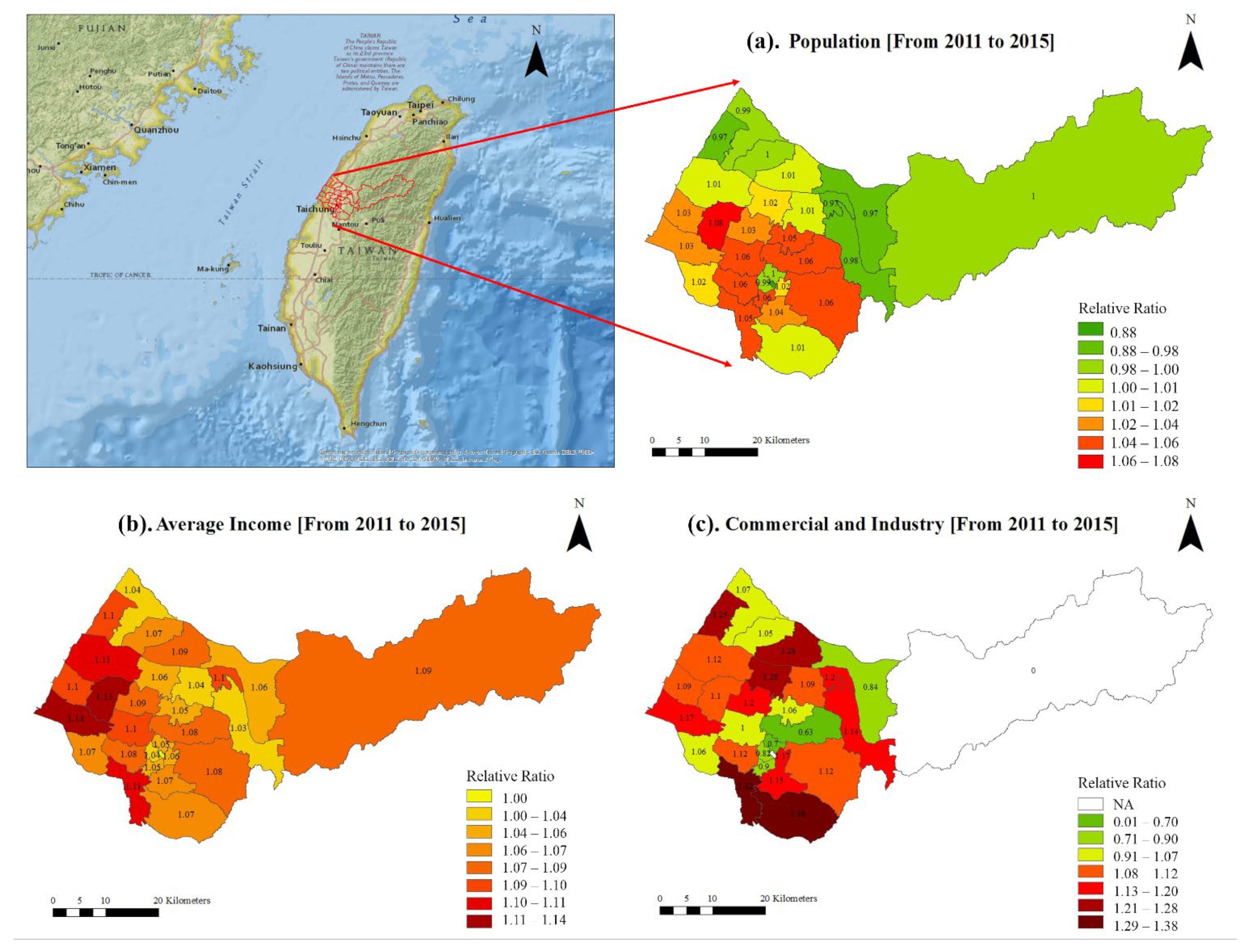
Figure 3.
Cluster map of energy and water consumption with LISA for year 2015 and 2017.
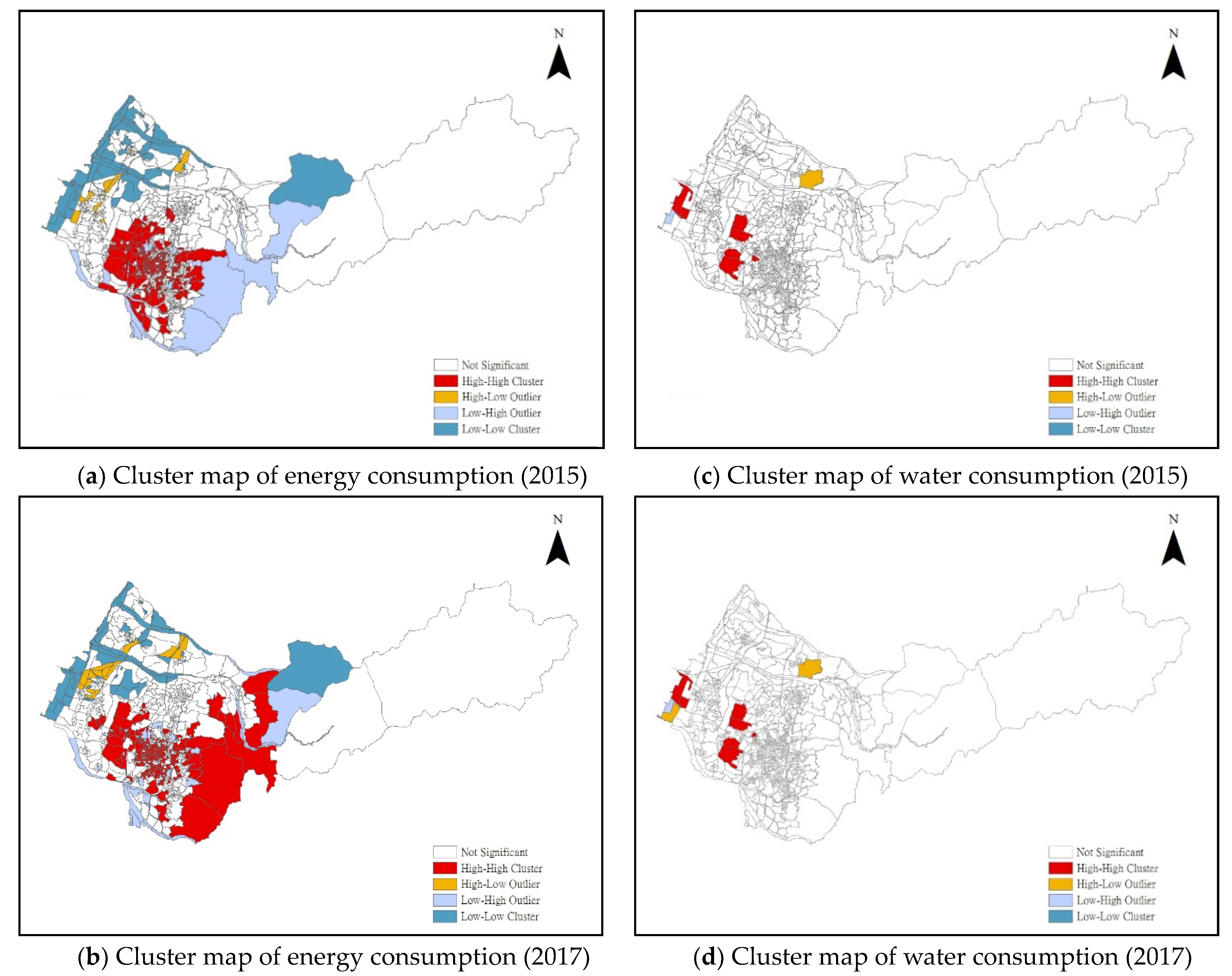
Figure 4.
Maps of residual on industrial energy and water consumption in GWR analysis.
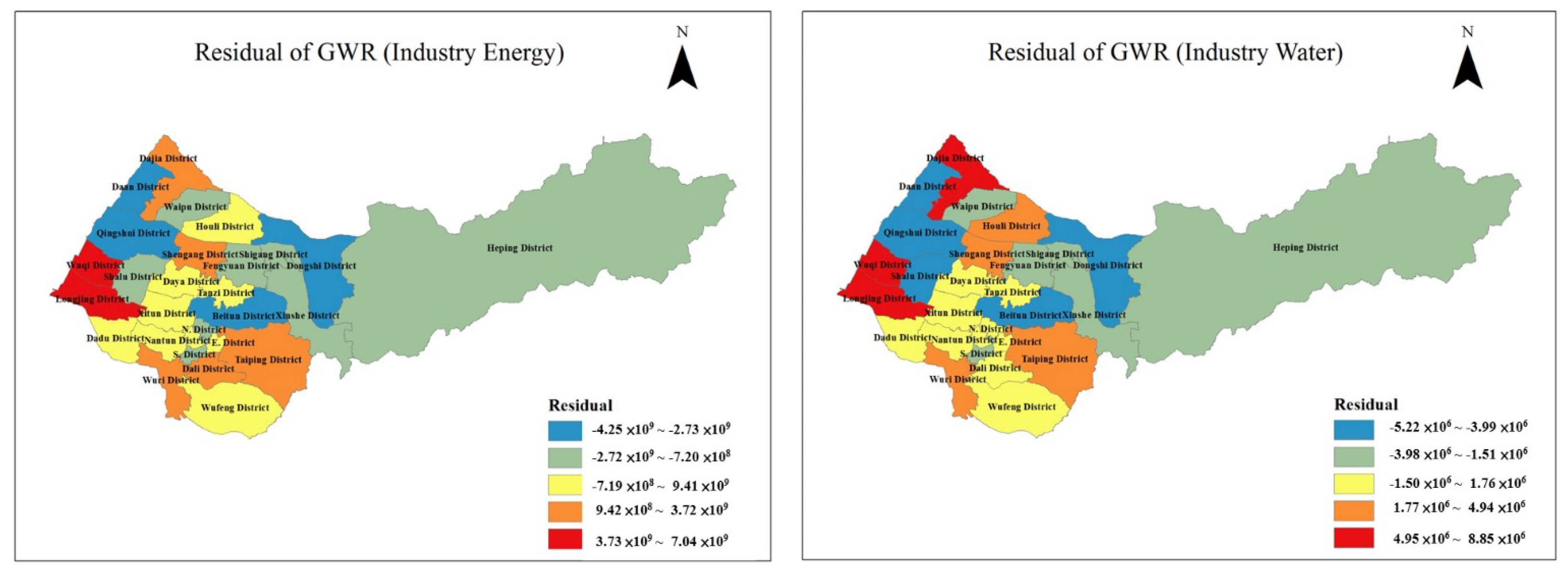
Figure 5.
Maps of residual on agriculture energy and water consumption in GWR analysis.

Figure 6.
Effects of independent variables on domestic energy and water consumption.

Figure 7.
Comparison of analyzed results and real data for the energy consumption in ratio.
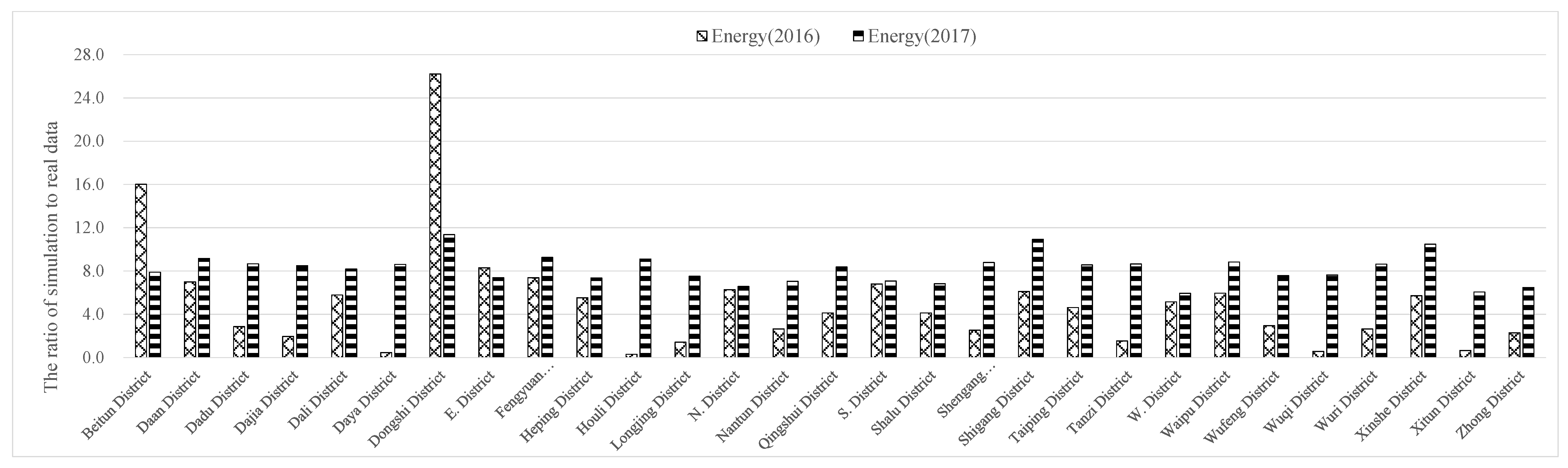
Figure 8.
Prediction maps of increased ratios of the independent variables in 2030 and 2050. Note: relative ratio = Xi,2030 (2050)/Xi,2015; I = number of population, average income, or enterprises.
Figure 8.
Prediction maps of increased ratios of the independent variables in 2030 and 2050. Note: relative ratio = Xi,2030 (2050)/Xi,2015; I = number of population, average income, or enterprises.

Table 1.
Filtered results of socio-economic variables with OLS in 2015.
| Item | Independent Variables | VIF | Domestic Energy | Industry Energy | Agriculture Energy | Domestic Water | Industry Water | Agriculture Water | ||||||
|---|---|---|---|---|---|---|---|---|---|---|---|---|---|---|
| Economic | Average income (NTD/Household) | 3.60 | * | * | * | |||||||||
| Number of enterprises | 6.69 | * | * | * | * | |||||||||
| Social | Population | 200.68 | * | * | * | * | ||||||||
| Building attributes | Three room units | 20.00 | * | * | ||||||||||
| More than six room units | 127.95 | |||||||||||||
| Floor area (m2)-Light Steel | 9.73 | * | * | * | ||||||||||
| Floor area (m2)-Steel Concrete | 2.89 | * | * | |||||||||||
| AIC | R2 | AIC | R2 | AIC | R2 | AIC | R2 | AIC | R2 | AIC | R2 | |||
| 1006.44 | 0.999 | 1354.67 | 0.377 | 1174.85 | 0.169 | 729.98 | 0.999 | 984.02 | 0.252 | 1113.02 | 0.230 | |||
Note: * an asterisk next to a number indicates a statistically significant p-value (p < 0.05).
Table 2.
Energy consumption results from GWR model for 2015.
| Sector | AIC | Local R2 | Enterprise Coeff. | Avg. Income Coeff. | Population Coeff. | Steel Concrete Coeff. | Light Steel Coeff. |
|---|---|---|---|---|---|---|---|
| Domestic | 1000.56 | 0.999 | 6160.94 | 9729.97 | 13,222.51 | 2.48 | - |
| Industry | 1356.15 | 0.347 | 502,635.40 | −10,882,891.85 | 40,707.19 | 40,707.19 | −9724.41 |
| Agriculture | 1152.54 | 0.420 | −8425.81 | −210,024.51 | - | - | 2696.73 |
Note: geographic information for no. of rooms is not available and hence not included in GWR analysis.
Table 3.
Water consumption results from GWR model for 2015.
| Sector | AIC | Local R2 | Enterprise Coeff. | Avg. Income Coeff. | Population Coeff. | Steel Concrete Coeff. | Light Steel Coeff. |
|---|---|---|---|---|---|---|---|
| Domestic | 723.50 | 0.999 | 53.19 | 67.20 | 112.47 | 0.01 | - |
| Industry | 981.90 | 0.308 | 1254.04 | −16,057.21 | 58.19 | 5.32 | −17.71 |
| Agriculture | 1104.03 | 0.294 | 877.50 | −111,178.96 | - | - | 125.14 |
Note: geographic information for no. of rooms is not available and hence not included in GWR analysis.
Table 4.
Comparing results between study analysis and real monitoring data for water consumption.
| District | Beitun | Daan | Dadu | Dajia | Dali | Daya | Dongshi | E. | Fengyuan | Heping | Houli | Longjing | N. | Nantun | Qingshui |
| Water(2016) | 0.95 | 5.99 | 1.38 | 1.24 | 1.19 | 0.47 | 1.40 | 0.95 | 1.06 | 5.39 | 0.53 | 0.24 | 0.75 | 0.74 | 1.48 |
| Water(2017) | 0.98 | 5.38 | 1.42 | 1.30 | 1.27 | 0.47 | 1.47 | 0.99 | 1.12 | 5.13 | 0.46 | 0.19 | 0.79 | 0.76 | 1.51 |
| District | S. | Shalu | Shengang | Shigang | Taiping | Tanzi | W. | Waipu | Wufeng | Wuqi | Wuri | Xinshe | Xitun | Zhong | |
| Water(2016) | 0.82 | 1.13 | 0.90 | 1.67 | 1.18 | 0.93 | 0.73 | 1.60 | 1.26 | 0.41 | 0.91 | 1.68 | 0.41 | 0.74 | |
| Water(2017) | 0.87 | 1.17 | 0.95 | 1.67 | 1.24 | 0.98 | 0.76 | 1.68 | 1.30 | 0.41 | 0.95 | 1.65 | 0.39 | 0.77 |
Table 5.
Relative ratio of resource consumption in 2030 and 2050.
| Township | Relative Ratio Compared to 2015 | Township | Relative Ratio Compared to 2015 | ||
|---|---|---|---|---|---|
| 2030 | 2050 | 2030 | 2050 | ||
| Beitun | 16% | 43% | S. | 17% | 43% |
| Daan | −8% | −20% | Shalu | 24% | 59% |
| Dadu | 4% | 13% | Shengang | 7% | 17% |
| Dajia | 9% | 44% | Shigang | −2% | 5% |
| Dali | 13% | 32% | Taiping | 17% | 43% |
| Daya | 11% | 27% | Tanzi | 18% | 81% |
| Dongshi | 28% | 161% | W. | −6% | −13% |
| E. | 7% | 18% | Waipu | 33% | 160% |
| Fengyuan | 7% | 25% | Wufeng | 4% | 12% |
| Heping | −14% | −14% | Wuqi | 8% | 22% |
| Houli | 18% | 78% | Wuri | 15% | 39% |
| Longjing | 11% | 35% | Xinshe | 7% | −1% |
| N. | 140% | 1462% | Xitun | 17% | 43% |
| Nantun | 17% | 42% | Zhong | −42% | −41% |
| Qingshui | 2% | 6% | Average | 13% | 84% |
Note: Relative ratio = Xj,2030 (2050)/Xj,2015; and j = annual resource consumption of year j.
Publisher’s Note: MDPI stays neutral with regard to jurisdictional claims in published maps and institutional affiliations. |
© 2021 by the authors. Licensee MDPI, Basel, Switzerland. This article is an open access article distributed under the terms and conditions of the Creative Commons Attribution (CC BY) license (https://creativecommons.org/licenses/by/4.0/).
Share and Cite
MDPI and ACS Style
Chen, I.-C.; Cheng, K.-L.; Ma, H.-W.; Hung, C.C.W. Identifying Spatial Driving Factors of Energy and Water Consumption in the Context of Urban Transformation. Sustainability 2021, 13, 10503. https://doi.org/10.3390/su131910503
AMA Style
Chen I-C, Cheng K-L, Ma H-W, Hung CCW. Identifying Spatial Driving Factors of Energy and Water Consumption in the Context of Urban Transformation. Sustainability. 2021; 13(19):10503. https://doi.org/10.3390/su131910503
Chicago/Turabian StyleChen, I-Chun, Kuang-Ly Cheng, Hwong-Wen Ma, and Cathy C.W. Hung. 2021. "Identifying Spatial Driving Factors of Energy and Water Consumption in the Context of Urban Transformation" Sustainability 13, no. 19: 10503. https://doi.org/10.3390/su131910503
Note that from the first issue of 2016, this journal uses article numbers instead of page numbers. See further details here.