Featured Application
Interpolation of pXRF assay data as a texture on a 3D model.
Abstract
The presentation of X-ray fluorescence data (XRF) assays is commonly restricted to tables or graphical representations. While the latter may sometimes be in a 3D format, they have yet to incorporate the actual objects they are from. The presentation of multiple XRF assays on a 3D model allows for more accessible presentation of data, particularly for composite objects, and aids in their interpretation. We present a method to display and interpolate assay data on 3D models using the PyVista Python package. This creates a texture of the object that displays the relative differences in elemental composition. A crested helmet from Tomb 1036 from the Casale del Fosso necropolis, Veii, Italy, is used to exemplify this method. The results of the analysis are presented and show variation in composition across the helmet, which also corresponds with macroscopic and decorrelation stretching analyses.
1. Introduction
The application of photogrammetry for the purpose of creating 3D models is widely applied in archaeology and heritage studies [1,2]. Models are used for a range of purposes which have traditionally fallen under the blanket term ‘visualization’ but also include analytical techniques (e.g., [2,3,4]). Likewise, portable X-ray fluorescence (pXRF) has been increasingly deployed in a range of contexts for analysis and interpretation of materials, including bronze [5,6]. One feature of non-destructive pXRF analyses is that individual assays are taken on relatively small areas of an object’s surfaces (usually a few mm2). Thus, a set of spatially discrete data points can be generated across a single object and used to assess compositional variation (e.g., [5,7]). Further, although 3D modelling and pXRF are readily applied on their own, the potential to combine them to enhance interpretation is largely unexplored. Here, we apply photogrammetric modelling and pXRF analysis together by interpolating the results of the pXRF analysis onto the photogrammetric model. The results are also assessed with decorrelation stretching of the photogrammetry model texture to further assist in the interpretation of the manufacture of an Etruscan crested helmet.
2. Context
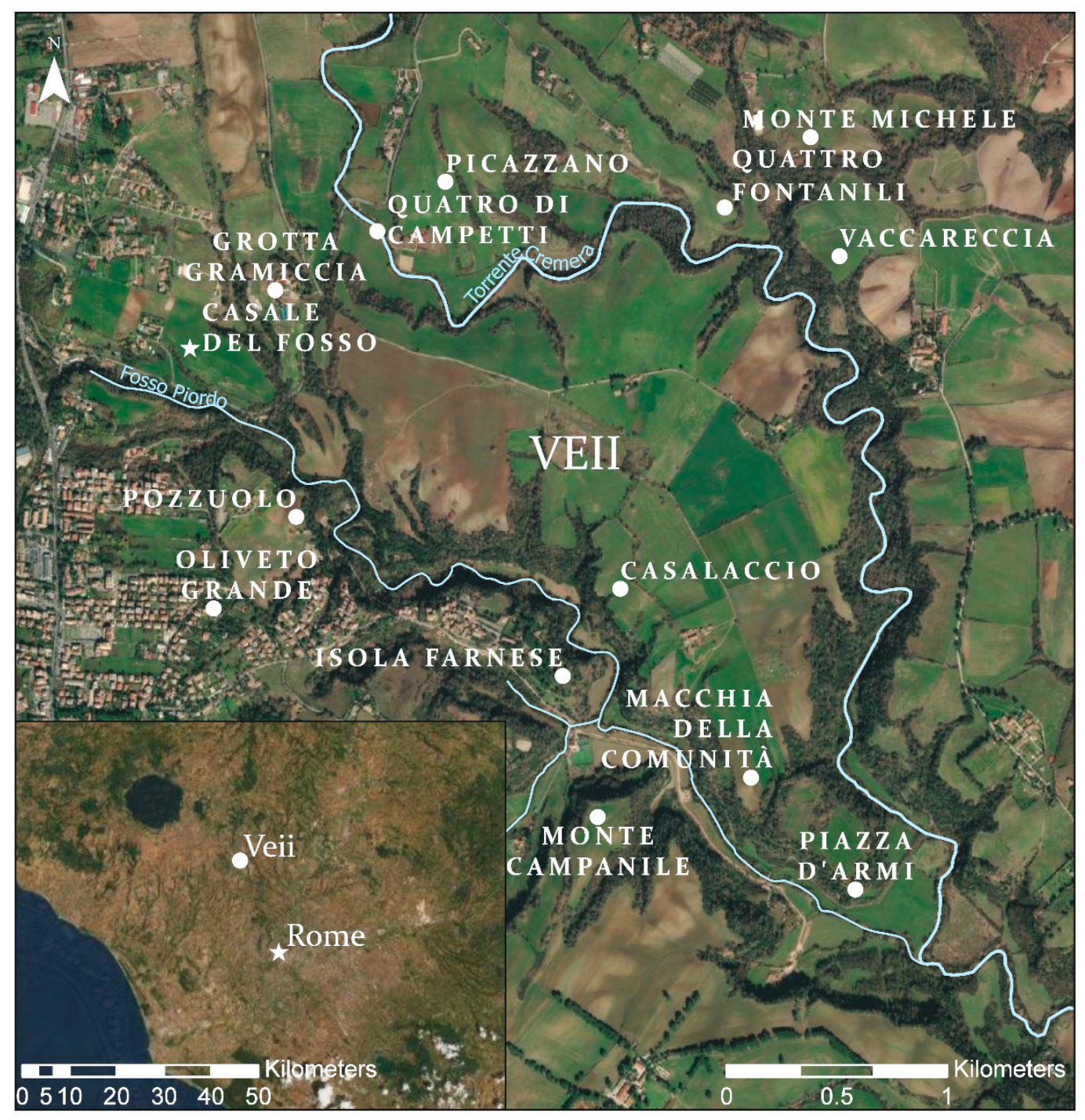
The crested helmet under investigation is from Tomb 1036 from the Casale del Fosso necropolis at Veii (Figure 1). The helmet is currently located in the Museo Nazionale Etrusco di Villa Giulia e Villa Poniatowski di Roma (National Etruscan Museum of the Villa Giulia and Villa Poniatowski in Rome) and was examined in January 2019. Veii, located approximately 15 km north-northwest of Rome (Figure 1), was an important community in southern Etruria, which flourished during the Italian Iron Age and was traditionally considered an early rival to Rome until its conquest in 396 BCE, according to the ancient literary evidence (Livy Ab Urbe Condita 5.22). Whether due to Roman conquest or not, the site went into decline around this time and remained mostly abandoned afterward, with brief periods of light occupation during the medieval period [8,9]. The urban centre of Veii is situated atop a plateau with the community’s various necropoleis surrounding it (Figure 1).
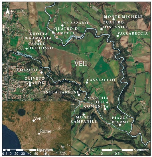
Figure 1.
The site of Veii with associated necropoleis, including the location of Casale Del Fosso.
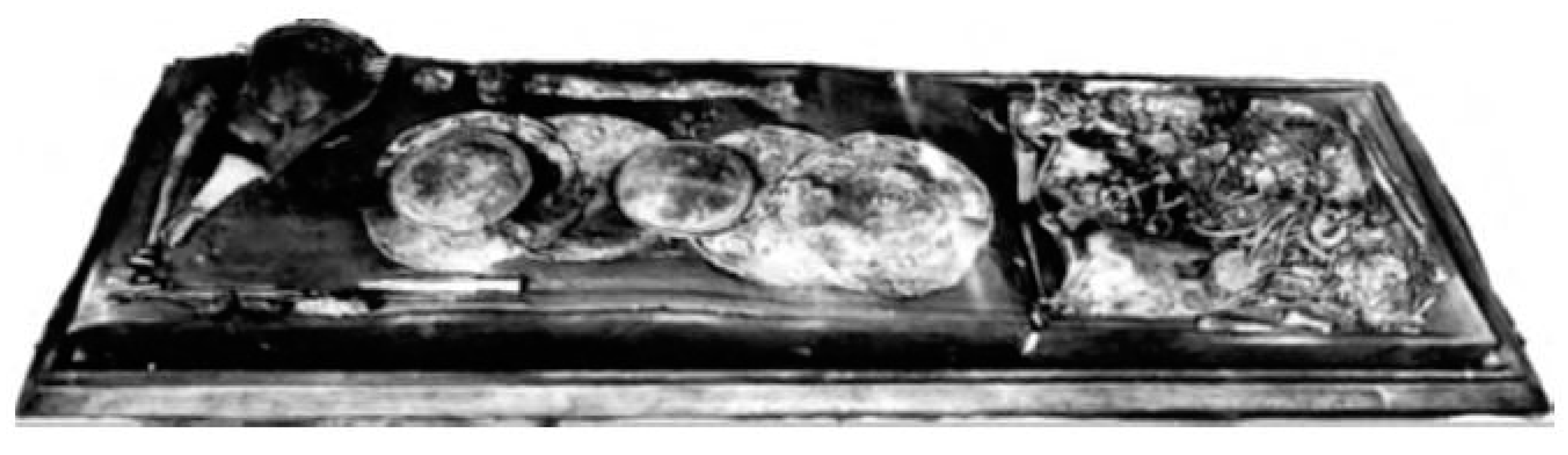
The site of Veii has been the subject of archaeological interest since the 14th century [10], although formal excavation only began in the 19th century and was initially focused on collecting valuable objects and worked marbles for private and museum collections. More systematic approaches were slowly adopted, and in the period between 1913 and 1918, a methodological investigation of several of the necropoleis was undertaken which uncovered around 1200 tombs from Grotta Gramiccia, Casale del Fosso, Pozzuolo, Monte Campanile, Valle La Fata, and Macchia della Comunità necropoleis [8,9]. Tomb 1036 from the Casale del Fosso necropolis, located to the northwest of the plateau (Figure 1), dates to between 750 and 731 BCE and was excavated in 1915. This grave was, from its initial discovery, understood to be exceptional due to both the style of burial and the number and the perceived quality of the grave goods. The context was a single inhumation burial, where the body was deposited into a fossa, or pit grave, in a wooden box which also contained grave goods. The grave goods included a spear, a pair of swords, a ‘mace’, a pair of composite ‘shields’, several large embossed bronze discs placed over the body, and this helmet. When excavated, the entire assemblage, including the body, the items, and the box, was encased in a thick layer of plaster and transported to the Villa Giulia in Rome to be conserved; due to a delicate conservation process, the finds were only displayed nearly a century later [11] (Figure 2).

Figure 2.
Contents of tomb 1200 after the removal of plaster. After Boitani [11]: 112.
The crested helmet from Tomb 1036 is of the ‘Villanovan-type’ [12], which emerged in Italy during the 9th century BCE, with the first examples appearing at Tarquinia—a nearby community in south Etruria. Although possibly connected to earlier crested helmets from continental Europe, such as the Pass-Lueg helmets of the Bronze Age, and with clear connections to helmets found in San Canziano-Škocjan, Hallstatt, and Zavadintsy, these crested helmets were evidently new to Italy in this period and quickly formed an important expression of the emerging ‘warrior ethos’, which is argued to have dominated amongst the elite within Etruria at this time [13]. By the late 8th century BCE, when this helmet was deposited, these types of helmets seem to have taken on increasing symbolic connotations—only associated with burials of the highest status [14].
The helmet, as with others of its type, was made through an elaborate process. The two halves (front and back in Figure 3) were likely formed by ‘sinking’, where a flat sheet is curved by hammering into a concave indentation. The vast majority of the decoration, which was likely achieved through repoussing or punching from the inside (most notably a series of small dots, largely invisible now due to patination), would have been added during this phase as well, as it would have been impossible to achieve once the helmet was assembled. Once both halves of the helmet were complete, they were placed together and connected with three rivets along the crest—one at the forehead, one at the crown, and one at the nape. Two cast plates, each with three prongs, were then attached to the forehead and the nape, adding further decorative elements and structurally binding the various pieces together. The helmet, therefore, contains at least four distinct pieces of bronze (the two halves and the two cast plates for the forehead and the nape) and at least three rivets; the cast plates on the forehead and the nape likely contain rivets as well, although this is uncertain. Finally, an organic band (leather or textile) would have been wrapped around the lower section of the helmet.
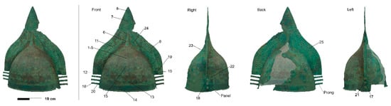
Figure 3.
Photogrammetry model with the different sides of the helmet shown and location of the pXRF assays on VG015 (numbers).
While the basic construction of the helmet is evident from a visual examination, the specific details of its production are largely unexplored. It is clear that the majority of the helmet was planned out in detail before construction began. However, at present, we do not know whether the casting of the blank sheets for the two halves of the helmet, the plates for the forehead and the nape, and the rivets occurred using the same alloy. If they are all the same alloy, it suggests the entire item was produced in a single workshop where there were at least two different types of bronze work occurring, hammering and casting, which involve two distinct skill sets and sets of resources. Alternatively, if the pieces are composed of slightly different alloys, that would support the possibility that the pieces were cast and created separately. This does not preclude them all being produced in the same workshop, although it would suggest a different chaîne opératoire—and indeed one which might involve a more complex set and sequence of relationships.
All of this obviously has implications for both the role and the production of bronze items in southern Etruria. ‘Villanovan-type’ crested helmets were transregional artefacts which, as Iaia suggested, served as important ‘vectors of technological and cultural transmission beyond their local region’—being found as far east as Fermo on the Adriatic coast and as far south as Capua and Sala Consilina in Campania and in the Piemonte region in the north [14]. It is also worth noting that southern Etruria, where this item was found, is not a mineral-rich area, and it is likely that the copper for it came from northern Etruria, in the so called ‘Etruria Mineraria’ (especially the Colline Metallifere north of Grosseto). Further, and as noted above, these helmets can be plausibly connected to both earlier crested helmets and contemporary finds from Europe, hinting at a vast social, cultural, economic, and technological network. Understanding how the specific production of an individual piece operated within this network can give vital clues about the nature of Etruscan society in this period.
3. Analyses
The combination of 3D data with methods which have been traditionally considered in isolation is becoming more common. Ultrasonic pulse velocity (UPV) testing and near-infra-red (NIR) imaging have been combined with 3D model to provide alternative visualization techniques to assess preservation in stone objects [15,16]. In other cases, more data are being extracted from 3D models themselves. For instance, Pfeuffer and colleagues used 3D laser scanning to measure surface roughness on stone sculpture as a way to inform on suitable preservation measures [17]. In another example, as part of the wider ‘Blood and Money’ project this paper is part of, the 3D thickness of a different helmet was measured as a way to assess manufacturing techniques [3]. This latter method, unfortunately, is not possible on the crested helmet discussed here, as it was not logistically practical to capture an accurate 3D model of its interior surface.
To investigate the general construction techniques of the crested helmet, several methods of analysis were employed—primarily, portable X-ray fluorescence (pXRF) to characterize the elemental composition and decorrelation stretching to show potential differences in colour. The results of the pXRF analysis were plotted onto a photogrammetric model of the helmet and interpolated, which forms another level of analysis. The interpolation of pXRF data as a texture for the 3D model allows for a more integrated approach to the analysis of composite objects than is commonly considered, where composite data are often presented visually separate from the object they are from (e.g., [18]). Therefore, interpolation of pXRF data provides an alternative way of visualizing results. Finally, decorrelation stretching was undertaken on the 3D model texture to potentially provide another means of identifying the various components of the helmet.
3.1. Photogrammetry
Following Emmitt et al. [3], the setup for the photogrammetry consisted of a light tent surrounded by five LED lights on tripods, a Bluetooth controlled turntable with a custom foam stand placed over it, and photogrammetry targets printed from Agisoft Metashape 1.5.3 [19]. Twenty-five images were taken around the object per rotation, with nine rotations done at different angles for a total of 225 photos of the helmet plus one image of the background to use as a mask during model construction. A Canon EOS 7D with a Canon EF 50m f/2.5 Macro lens was used for the photographs. Colour correction was done with an X-Rite Color Checker Photo Passport 2 [20,21]. The colour checker was photographed at the start of each set-up. Raw photographs were processed as digital negatives (DNG) in ColorChecker Passport and Adobe Lightroom Classic CC with the ColorChecker Passport plugin and JPG files for photogrammetry. Agisoft Metashape 1.5.3 [19] was used for the model creation. Blank images of the workspace were used to a create masks of the helmet. The constructed sparse point cloud was edited with the following parameters: reprojection error: 0.2 px; reconstruction uncertainty: 15 px; image count: 2; projection accuracy: 2.5 px. Editing of the dense cloud was done manually with some automation based on colour where possible. A mesh was generated over the object, and a texture was created. Where required, a reflexive method of deleting stray points on the dense cloud and re-generating the mesh and the texture was conducted. The final photogrammetry model is available as part of the dataset of Emmitt and colleagues [22] (Figure 3). Due to logistical constraints, only the exterior of the helmet was modelled, thus thickness analyses, such as those done in Emmitt and colleagues [3], were not possible.
3.2. pXRF
Following Emmitt et al. [6], we used a Bruker Tracer III-SD portable X-ray Fluorescence (pXRF) analyser (Bruker, Billerica, MA, USA; also see Appendix A). The instrument employs an X-ray tube with an Rh target and a 10 mm2 silicon drift detector (SDD) with a typical resolution of 145 eV at 100,000 cps. For analysis of copper-based alloys, we found that operating the X-ray tube with a setting of 40 keV at 5.0 μA in an air-path and through a window composed of 12 mil Al and 1 mil Ti filters (Bruker’s Yellow filter) provided a good count rate for the elements of interest. Assays of artefacts were taken for 60 s each, and their locations were recorded on annotated photographs and transcribed to a photogrammetric model of each object. Reference standards were analysed using the same machine and settings outlined above (Appendix A). Each standard was analysed twice for 60 s, and the results were averaged.
In total, 25 assays were taken on the helmet (Figure 3). The assay locations were selected based on a subjective assessment of the object, which included the visually determined position of different physical features, such as decorative elements, rivets, and areas potentially less affected by patina than others. Assays 1–5 formed a ‘cluster assay’, which took the average of the results of five assays over a 1 cm diameter area (Figure 4). The aim of the cluster assay was to provide a more representative sample in an area that was considered less affected by patina formation. The order the five assays were recorded in is presented in Figure 4. The cluster assay measures variation over a relatively contained surface area, where both the core metal and the depositional conditions should be largely consistent [6]. This type of approach falls into the category of ‘area mapping’, as proposed by Karydas et al. [23], to ascertain mean values of elemental intensities across an area and address the issue of microscale heterogeneity common on bronze alloys. Assays were targeted at the cleanest areas possible (i.e., those with perceived low surface roughness caused by patina). Calibrated results from the analysis are presented in Table 1.
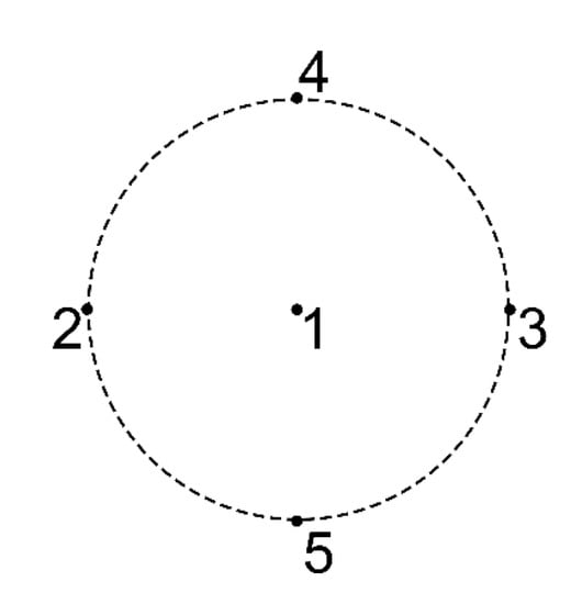
Figure 4.
Example of the order in which cluster assays were taken over a 1 cm diameter circle.
In addition to the calibrated assays, the Compton scatter is also useful for analysis. The inelastic Compton scatter of the X-ray target (Rh in this case) is inversely proportional to the mean atomic weight of the sample and therefore provides a measure for the relative density of the sample area (see [24]).

Table 1.
Calibrated data for assays used in the analysis. Assays 1–5 are reported as the average values of the cluster. Additionally shown are the count rates (counts per second) for the inelastic Compton scatter of the Rh target (integrated over a range of 18.5–19.5 keV).
Table 1.
Calibrated data for assays used in the analysis. Assays 1–5 are reported as the average values of the cluster. Additionally shown are the count rates (counts per second) for the inelastic Compton scatter of the Rh target (integrated over a range of 18.5–19.5 keV).
| Assay | Location | Mn % | Fe % | Ni % | Cu % | Zn % | As % | Sn % | Sb % | Pb % | Compton cps |
|---|---|---|---|---|---|---|---|---|---|---|---|
| 1–5 | Front | 0.049 | 0.440 | 0.150 | 59.1 | 1.21 | 1.01 | 20.2 | 0.295 | 2.74 | 174.7 |
| 6 | Front | 0.057 | 0.401 | 0.118 | 55.0 | 1.30 | 0.68 | 17.2 | 0.232 | 1.69 | 172.9 |
| 7 | Front | 0.048 | 0.495 | 0.165 | 48.2 | 1.43 | 0.75 | 22.8 | 0.302 | 2.06 | 180.0 |
| 8 | Front | 0.048 | 0.442 | 0.138 | 51.9 | 1.48 | 0.76 | 23.3 | 0.329 | 2.15 | 179.6 |
| 9 | Front | 0.050 | 0.416 | 0.157 | 53.8 | 1.27 | 0.60 | 17.5 | 0.210 | 1.86 | 157.2 |
| 10 | Front | 0.046 | 0.474 | 0.191 | 42.9 | 1.66 | 0.63 | 22.8 | 0.309 | 1.91 | 157.5 |
| 11 | Front | 0.047 | 0.405 | 0.138 | 51.9 | 1.37 | 0.68 | 22.4 | 0.297 | 2.13 | 166.6 |
| 12 | Front | 0.051 | 0.524 | 0.195 | 45.4 | 1.72 | 1.30 | 35.8 | 0.441 | 3.79 | 215.1 |
| 13 | Front | 0.048 | 0.416 | 0.123 | 54.0 | 1.15 | 0.75 | 20.0 | 0.300 | 2.83 | 170.2 |
| 14 | Front | 0.047 | 0.388 | 0.197 | 42.5 | 1.34 | 0.80 | 20.1 | 0.276 | 2.18 | 154.7 |
| 15 | Front | 0.048 | 0.485 | 0.182 | 55.7 | 1.35 | 1.10 | 24.4 | 0.299 | 2.87 | 183.7 |
| 16 | Prong | 0.046 | 0.360 | 0.210 | 38.9 | 1.47 | 0.73 | 14.5 | 0.283 | 2.63 | 129.6 |
| 17 | Prong | 0.450 | 0.284 | 0.202 | 36.7 | 1.50 | 0.16 | 3.70 | 0.057 | 0.45 | 72.4 |
| 18 | Panel | 0.049 | 0.380 | 0.166 | 48.1 | 1.22 | 0.45 | 17.4 | 0.228 | 1.56 | 157.8 |
| 19 | Rivet | 0.050 | 0.601 | 0.167 | 48.3 | 1.56 | 0.79 | 26.3 | 0.366 | 2.19 | 191.2 |
| 20 | Prong | 0.048 | 0.403 | 0.206 | 42.8 | 1.61 | 1.17 | 21.5 | 0.407 | 3.99 | 162.6 |
| 21 | Panel | 0.047 | 0.309 | 0.185 | 45.0 | 1.29 | 0.77 | 14.2 | 0.212 | 3.01 | 136.6 |
| 22 | Prong | 0.048 | 0.577 | 0.167 | 47.2 | 1.49 | 0.55 | 19.6 | 0.361 | 2.54 | 155.5 |
| 23 | Back | 0.055 | 0.366 | 0.106 | 63.2 | 0.79 | 0.61 | 26.7 | 0.439 | 1.55 | 192.3 |
| 24 | Front | 0.045 | 0.408 | 0.159 | 46.8 | 1.46 | 0.50 | 14.5 | 0.178 | 1.09 | 140.9 |
| 25 | Back | 0.047 | 0.365 | 0.181 | 47.8 | 1.21 | 0.67 | 25.6 | 0.412 | 1.85 | 172.0 |
3.3. D Assay Interpolation
Display of the assays on the 3D model was achieved by first selecting the assay locations as points in Blender v2.90.1. This was done by manually selecting the point locations on the helmet by comparing to photographs taken during data acquisition. These points were exported as a .csv file, which included their locations relative to the rest of the model (script included with supplementary data [22]). The pXRF data were related to the point locations in the .csv format. The point values were then interpolated onto the model using the PyVista toolkit v0.28.1 [25]. The field used for interpolation could be selected from those in the .csv file thus may have been any of the pXRF results or any other desired variable. PyVista uses a Gaussian kernel interpolation, which applies the values to the area within a specified radius of the point on the mesh. The code script and the data were included in the data repository for this paper [22]. The presentation in the Juypter notebook included in the data also provided a view in 3D of the interpolated model.
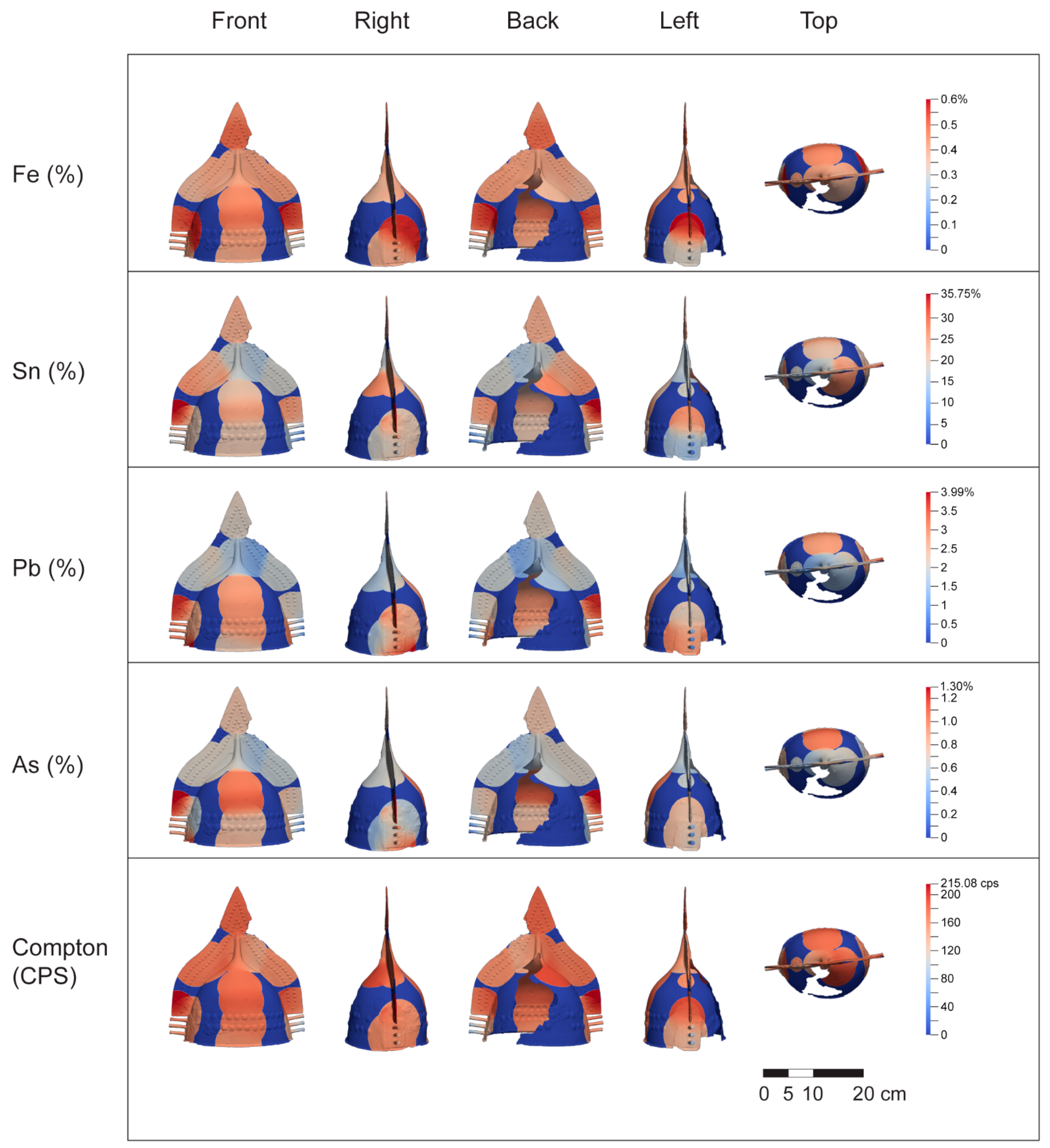
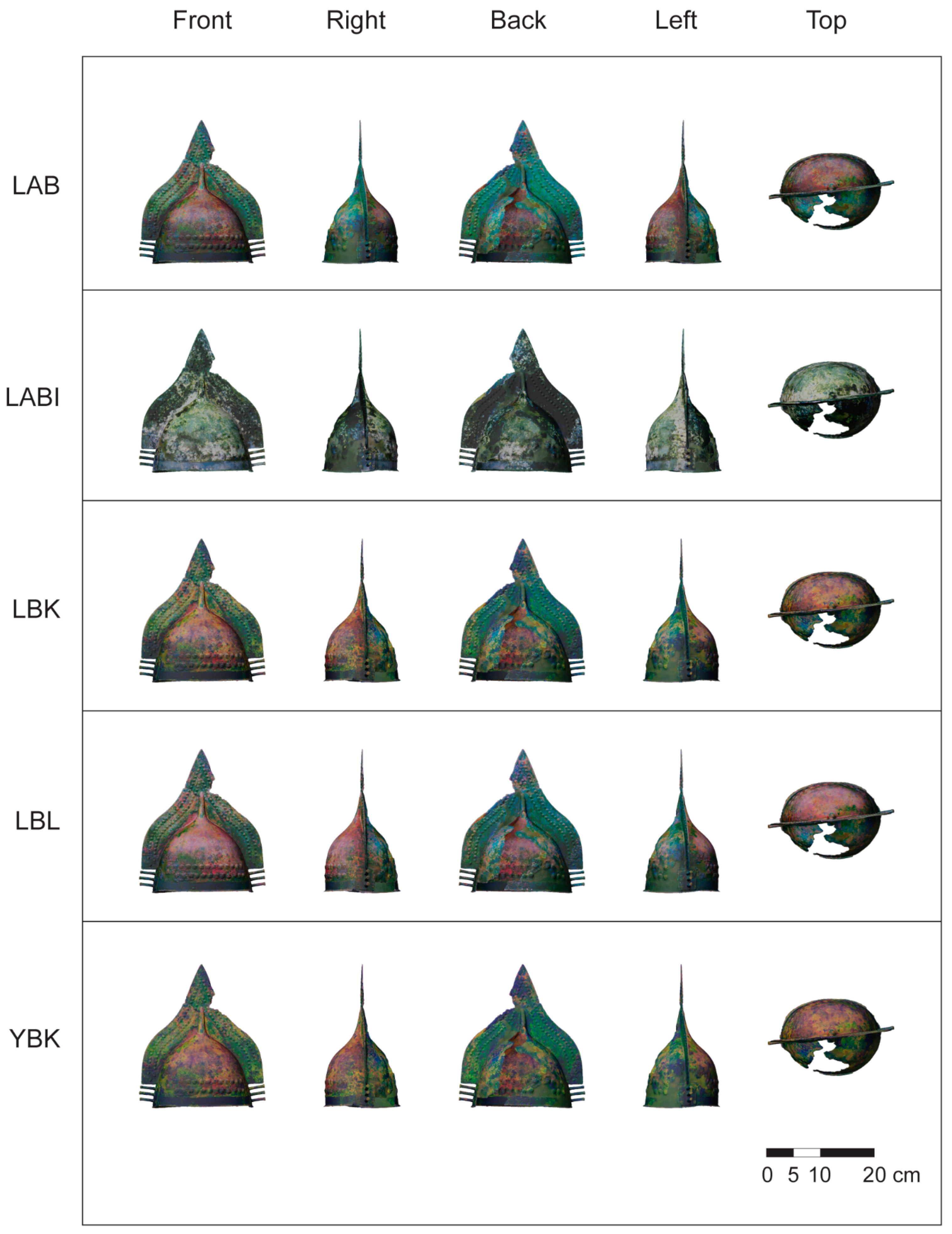
In Figure 5, we display views of the helmet with interpolation values of the pXRF analysis we determined as the most useful for examining the helmet, those being Fe, Sn, Pb, As, and the Compton values. The colours for each element were designated based on the maximum value, which is red in Figure 4. As there were no elements with a measurement of zero, the colour blue was treated as a null value and was also the minimum value on the scale. The interpolations were conducted at a radius of 5 cm so as to allow some blending of values while not over-representing the assay data on the object. As the search radius was 5 cm and the helmet was much thinner than that, in some cases under 1 mm, it did not distinguish well between different sides, which has implications for the interpretation of the different sheets the helmet is made from, as we discuss further below. However, it did provide an indication of the composite nature of the helmet as it presently exists, which is the result of both the initial production techniques and the post-depositional factors—most notably patination.
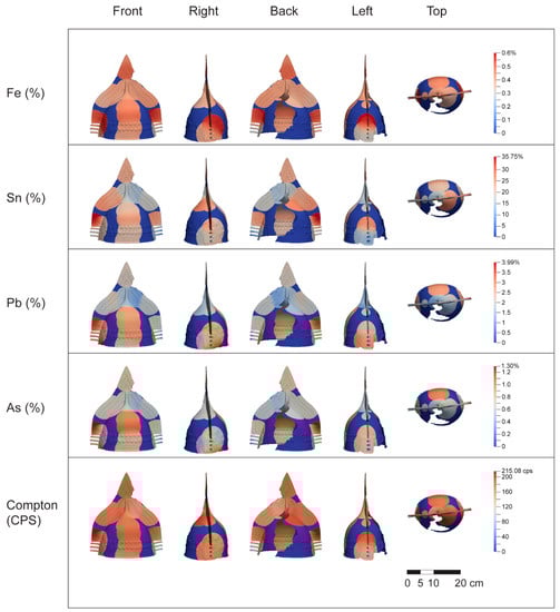
Figure 5.
Interpolated values of the pXRF analyses onto the photogrammetric model.
The results of the interpolation demonstrate differences in the composition of the helmet. While, at first glance, it appears relatively homogenous, there are clearly differences between the crest and the bowl of the helmet and again towards the rim. Much of this difference almost certainly relates to variable patination processes, as the crest and the bowl of the helmet, on each side, are known to come from a single piece of hammered bronze. This is reinforced by the fact that the two halves of the helmet, which are made from separate pieces of bronze, seem to share broad similarities. Iron is present throughout the helmet but is higher on the rivet and towards the base of the crest. Lead is present in a higher proportion on the rivet but also along the main body of the helmet. The Compton results further demonstrate the relative homogeneity of the helmet with the exception of the prongs visible on the left view in Figure 5, which display a lower proportion of the elements displayed and a relatively lower density.
3.4. Decorrelation Stretch
The final method of analysis applied to the helmet was decorrelation stretching through the use of the DStretch [26,27] plugin for the image processing software Image-J [28]. Decorrelation stretching exaggerates the colour separation of an image and was selected as it could be applied to already available data, mainly the texture generated for the photogrammetry model. The colorspace algorithms were selected based on those that displayed the most visual distinction (Figure 6). The most distinct variation was identified at the darker end of the hue spectrum, which was also the case for pigments in rock art [29]. Distinctions were identified over some parts of the model. For instance, the colorspace LABI identified one side as more heavily patinated than the other, with the patina showing up in white. This likely relates to the way it was deposited in the tomb and later preserved in plaster, lying on its side, and also likely contributed to the differential preservation of the helmet, with one side (Back view in Figure 6) featuring significantly more damage than the other.
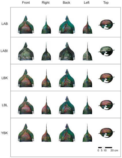
Figure 6.
Results of the decorrelation stretch analysis by colorspace.
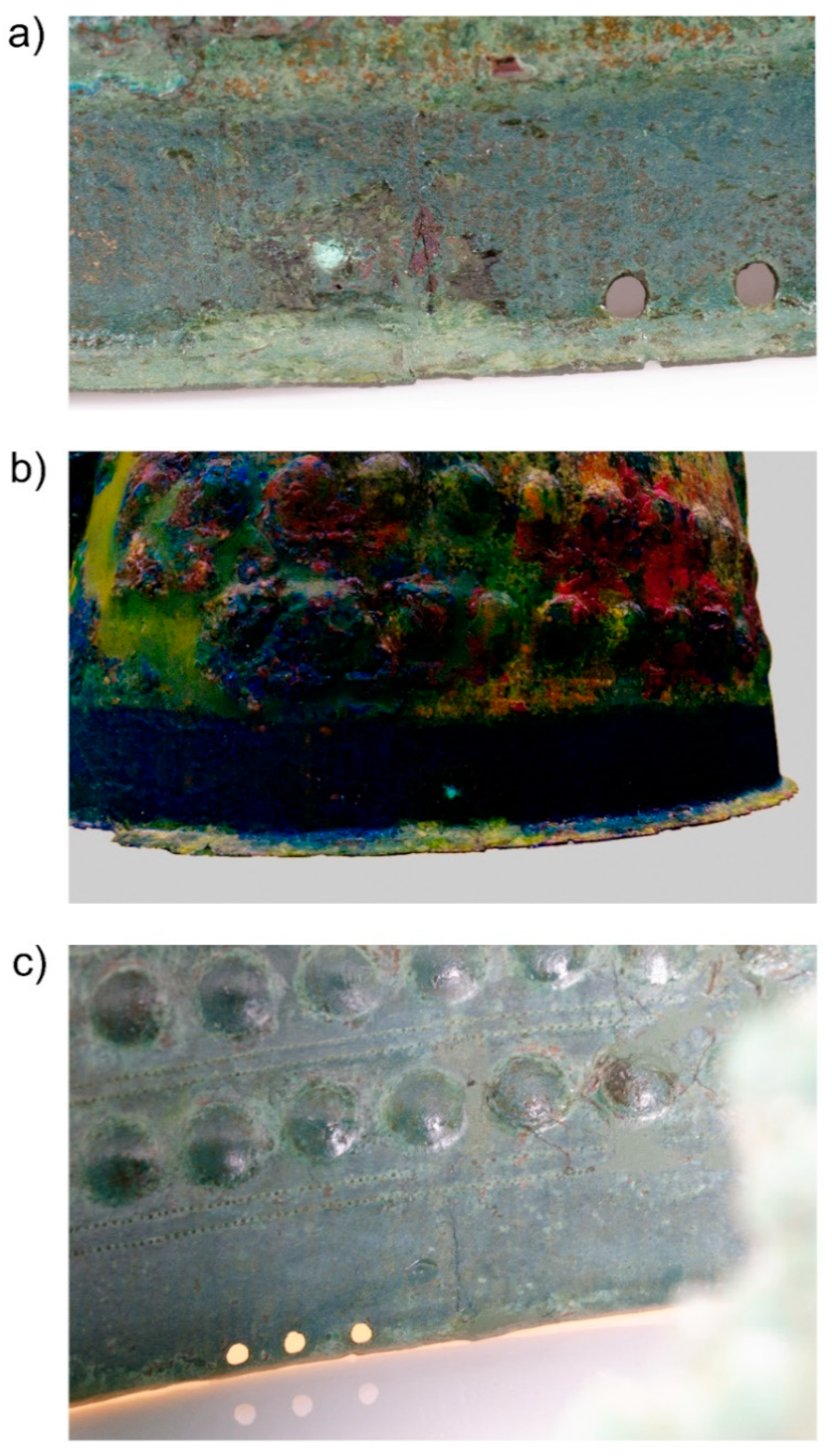
Additionally, the decorrelation stretching highlighted a band around the lower segment of the helmet, which seemed to be covered in an organic element that disappeared. This band is visible to the naked eye (Figure 7a), although it lacks definition. The decorrelation stretching clearly revealed that the band originally went all the way around the helmet, even covering the plates at the forehead and the nape (Figure 7b). The fact that the band seemed to cover the plates, which included circular design elements (one of which may have been associated with a rivet), hints that it was a later addition and was perhaps not planned at the outset (Figure 7b). It should also be noted that space for a band was left on the bowl of the helmet, which was otherwise richly decorated with repoussed and punched features (Figure 7c). This reveals details about how the item would have looked in antiquity, visibly combining organic and metal elements on the exterior in addition to the organic elements which were likely present on the inside and the chinstrap.
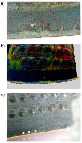
Figure 7.
(a) Banding visible in the pantina near the rim of the helmet (darker green area). (b) DStrech (LBK) view of the banding (in dark blue). (c) Detail of intricate decoration visible from the interior of the helmet.
4. Discussion
When viewed on the interpolated surface, the pXRF data presented above suggest that the entire helmet was produced from a single type of high-tin bronze alloy. Key differences in the measurements are either within a single piece of metal or cross the boundaries between them, indicating they are due to patination, other post-depositional processes, variable thickness of the piece (visible in the Compton value), or the natural variation present in ancient bronze. Thus, we can say that all four of the main pieces of bronze (the two halves as well as the forehead and the nape plates) are of a consistent composition. This, when combined with the consistency and the planning visible in the decoration, indicates that the helmet was most likely the product of a single workshop and was produced in what can be considered a relative ‘single event’. This is significant, as it indicates the presence of a complex workshop in the 8th century BCE able to handle large pours of metal into various shapes (sheets and more complex lost wax forms) as well as to perform the skilled hammerwork needed to finish the helmet.
The variations in the patina of the item are also useful. With regard to the ancient item itself, the band of discoloration likely associated with a (now lost) organic band first reveals the presence of a decorative element which was previously unidentified. Further, as the band seemed to cover elements of cast decoration, it is possible that, while the basics of the helmet’s decorative scheme were established in the initial casting phase, changes could be made later—perhaps in a different/associated facet of the chaîne opératoire associated with organic materials.
With regard to the item’s post-depositional history, the variations highlighted by the decorrelation stretching hint at how each side of the helmet was exposed to different conditions, which resulted in different patinas. The damaged side (back in Figure 3 and Figure 5) was likely the one left exposed upwards during deposition, with the more patinated side (front) remaining relatively protected but also exposed to patination forming processes over time. This was also confirmed by the position of the helmet in the tomb (Figure 2).
Such interpretations as those made here are possible by examining the assay data and comparing them to photographs or a 3D model of the helmet. However, the 3D interpolation utilized here offers a replicable means of visualizing these interpretations. It also provides a more complete view of the helmet. As we discussed elsewhere [6], it is vitally important that such items should be examined as more than single data points in wider assemblages and rather as objects of potential variation in themselves. The ability to position and interpolate other data sets on 3D models creates a more holistic approach to their interpretation.
Future applications of this method should focus on a systematic collection of data across an object. As the data used here were collected during a relatively short collection window as part of a larger project, it was only possible to collect a limited number of points. Ideally, the number of points should be spaced across the object and not necessarily in relation to the different parts of it. This requires a method for collecting data which has the pXRF locations marked as part of the image texture at acquisition as opposed to marking photographs of the object as assays are taken, which we admit creates a larger margin for error than may otherwise be the case.
5. Conclusions
With exception to the photogrammetry software used (for which there are open-source alternatives), the methods employed here utilize open-source toolkits for preparation, analysis, and presentation of the 3D data. These data are published in an open repository where they can be downloaded and viewed. The technique discussed also enables others to re-run the interpolation tools we used in the paper and replicate the results of the analysis.
The results here highlight the need to consider multiple lines of evidence when examining composite objects in general, and bronzes in particular, and also the benefits of considering assays holistically and in a 3D context. Alone, the pXRF results can be presented on a table, and conclusions, such as those reached here, could have been achieved without the 3D interpolation. However, we would argue that such results are enhanced and rendered more accessible through their presentation on a 3D model. Most notably, the relationship between the points assayed as well as their relative positions on the artefact are often missed or can be misinterpreted when presented as simple tabular data. For instance, when considering the helmet discussed in this paper, the evident variability in the readings can be contrasted with the visible structuring of the helmet, its two halves and two plates, making analysis and interpretation much easier. Variability within and across different pieces is quickly and clearly evident, revealing that the most substantial variations likely relate to patination and not production. Comparisons using the Compton scatter measurements, both amongst the readings themselves and across calibrated elements, also highlight areas where, particularly on an item as thin as the helmet (c. 0.5 mm in places), additional care should be taken in interpretation due to the increased density which, at least in this instance, likely relates to thickness.
A particular benefit to the interpolation approach we propose is that it provides a visual aspect to the data which integrates them with their parent object. It also enables them to be readily compared to other visual analyses. For example, when compared against the DStretch models, another line of evidence is provided by which to interpret both the assays and the wider artefact. The photogrammetric model itself is used as a base in these cases as opposed to being limited to only a visualisation element. As 3D data and publishing become more integrated and complex (see [30]) so too do the possibilities for combining techniques that have traditionally not been considered complementary.
Author Contributions
Conceptualization, J.E. and J.A.; Methodology, J.E., A.M. and J.A.; Software, J.E.; Validation, J.E., A.M. and J.A.; Formal Analysis, J.E., A.M.; Investigation, J.E.; Resources, J.E. and J.A.; Data Curation, J.E.; Writing—Original Draft Preparation, J.E., A.M., N.B., J.A.; Writing—Review & Editing, J.E., A.M., N.B. and J.A.; Visualization, J.E.; Supervision, J.A.; Project Administration, J.A.; Funding Acquisition, J.A. All authors have read and agreed to the published version of the manuscript.
Funding
This study was funded by the Royal Society of New Zealand Marsden Fund project ‘Blood and Money: The “Military Industrial Complex” of Archaic Central Italy’ [17-UOA-136] awarded to Jeremy Armstrong.
Institutional Review Board Statement
Not applicable.
Informed Consent Statement
Not applicable.
Data Availability Statement
The calibrated assays used in this study are presented in Table 1. Photogrammetric models, decorrelation stretching textures, calibrated assays, and assay locations are available at: Emmitt, J., McAlister, A., Bawden, N. and Armstrong, J. (2021c) ‘3D and assay data published in ‘XRF and 3D modelling on a composite Etruscan helmet’’. Zenodo doi:10.5281/zenodo.5160531.
Acknowledgments
Thanks to Rebecca Phillipps for comments on this paper, Sina Masoud-Ansari for advice on implementing the scripts, and Seline McNamee for assistance with the preparation of the figures. Thanks is due to the director and the curators from the Museo Nazionale Etrusco di Villa Giulia e Villa Poniatowski di Roma for facilitating access to their collections, permitting publication of the resultant models and data, and allocating staff, space, and time to help us during our visit. In particular, we would like to thank Giulia Bison and Valentino Nizzo for their help. The work would also have been impossible without Jono Grose and Nic Harrison of Redoubt Forge, who operated the photogrammetry workstation and assisted with the macro photography.
Conflicts of Interest
The authors declare no conflict of interest.
Appendix A. Portable X-ray Fluorescence Calibration Procedures
In this study, we used a Bruker Tracer III-SD portable X-ray Fluorescence (pXRF) analyser. The instrument employs an X-ray tube with an Rh target and a 10 mm2 silicon drift detector (SDD) with a typical resolution of 145 eV at 100,000 cps. For analysis of copper-based alloys, we found that operating the X-ray tube with a setting of 40 keV at 5.0 μA in an air-path and through a window composed of 12 mil Al and 1 mil Ti filters (Bruker’s Yellow filter) provided a good count rate for the elements of interest. Assays of artefacts were taken for 60 s each, which was sufficient time to obtain stable results and was in line with other researchers using similar instruments [5,31,32]. Nine modern copper-based alloy reference standards were used for the calibration of these data (Table A1). Each reference standard was analysed twice, and the results were averaged.
Given the relatively small number of standards available, the calibration procedure was kept as simple as possible. Linear regressions on the net characteristic element peaks (normalised to counts-per-second) were employed, and corrections for interference peaks were included in the regression formulas where necessary (Table A2, Figure A1). For example, the escape Kα peak of Cu (6.306keV) overlaps with the characteristic Kα peak of Fe (6.405 keV) and introduces error if not accounted for in the regression equation.
In the case of three elements (Ni, Sb, and Pb), slightly negative values were occasionally obtained from the calibration. Examination of typical spectra indicates that, at low concentrations, the peaks for these elements are swamped by the tails of the much larger Cu, Kα, and Kβ peaks at low concentrations (Figure A2).
Table A1.
Reference standards used for the calibration with given values (%). Uncertified values are underlined. 1 Outlier removed from calibration.
Table A1.
Reference standards used for the calibration with given values (%). Uncertified values are underlined. 1 Outlier removed from calibration.
| Mn | Fe | Ni | Cu | Zn | As | Sn | Sb | Pb | |
|---|---|---|---|---|---|---|---|---|---|
| Given values | |||||||||
| BCR-691-A | 0.20 | 0.20 | 0.10 | 76.50 | 6.02 | 0.19 | 7.16 | 0.50 | 7.90 |
| BCR-691-B | 0.40 | 0.50 1 | 0.20 | 81.00 | 14.80 | 0.10 | 2.06 | - | 0.39 |
| BCR-691-C | 0.20 | 0.20 | - | 95.00 | 0.06 | 4.60 | 0.20 | 0.50 | 0.18 |
| BCR-691-D | 0.10 | 0.10 | 0.30 | 80.50 | 0.15 | 0.29 | 10.10 | 0.30 | 9.20 1 |
| BCR-691-E | 0.30 | 0.30 | 0.50 | 91.50 | 0.16 | 0.19 | 7.00 | 0.70 | 0.20 |
| MBH-32X PB11 | 0.04 | 0.37 | 0.72 | 92.09 | 1.60 | 0.19 | 3.20 | 0.47 | 1.08 |
| MBH-32X SN6B | 0.09 | 0.38 | 0.30 | 85.73 | 2.00 | 0.80 | 6.78 | 0.30 | 1.64 |
| MBH-33X 54400A | - | 0.07 | 0.24 | 86.79 | 3.87 | 0.02 | 3.97 | 0.04 | 4.69 |
| MBH-33X RB2 B | 0.08 | 0.50 | 0.33 | 82.02 | 9.01 | 0.04 | 4.65 | 0.05 | 2.99 |
| Calibrated values | |||||||||
| BCR-691-A | 0.17 | 0.21 | 0.07 | 78.21 | 5.72 | 0.19 | 6.72 | 0.46 | 8.00 |
| BCR-691-B | 0.42 | - | 0.25 | 85.34 | 15.10 | 0.11 | 2.04 | - | 0.43 |
| BCR-691-C | 0.21 | 0.20 | - | 96.21 | −0.01 | 4.62 | 0.10 | 0.54 | 0.25 |
| BCR-691-D | 0.10 | 0.11 | 0.29 | 79.50 | 0.46 | 0.30 | 9.79 | 0.27 | - |
| BCR-691-E | 0.27 | 0.32 | 0.48 | 86.63 | 0.31 | 0.19 | 7.40 | 0.68 | 0.22 |
| MBH-32X PB11 | 0.09 | 0.37 | 0.71 | 91.33 | 1.56 | 0.19 | 3.22 | 0.49 | 1.06 |
| MBH-32X SN6B | 0.11 | 0.34 | 0.34 | 83.00 | 2.00 | 0.72 | 7.14 | 0.34 | 1.75 |
| MBH-33X 54400A | - | 0.09 | 0.22 | 86.89 | 3.86 | 0.07 | 3.97 | 0.04 | 4.59 |
| MBH-33X RB2 B | 0.06 | 0.52 | 0.35 | 84.04 | 8.68 | 0.07 | 4.77 | 0.05 | 2.80 |
Table A2.
Calibration parameters. 1 Detection limit calculated as 3.3 * (σ/S).
Table A2.
Calibration parameters. 1 Detection limit calculated as 3.3 * (σ/S).
| Element | Conc. | R2 | RMS | Mean Abs. | Det. | Element | Interference |
|---|---|---|---|---|---|---|---|
| Range (%) | Error (%) | Error (%) | Lim. 1 | Peak | Corrections | ||
| Mn | 0.04–0.40 | 0.944 | 0.03 | 0.02 | 0.05 | Mn Kα1 | - |
| Fe | 0.07–0.50 | 0.989 | 0.02 | 0.01 | 0.06 | Fe Kα1 | Cu Kα1 (Escape peak) |
| Ni | 0.10–0.72 | 0.976 | 0.03 | 0.03 | 0.05 | Ni Kα1 | Cu Kα1 (Peak overlap) |
| Cu | 76.50–95.00 | 0.806 | 2.59 | 2.08 | 34.84 | Cu Kα1 | - |
| Zn | 0.06–14.80 | 0.998 | 0.21 | 0.17 | 0.24 | Zn Kα1 | Cu Kβ1 (Peak overlap) |
| As | 0.02–4.60 | 0.999 | 0.04 | 0.02 | 0.04 | As Kβ1 | - |
| Sn | 0.20–10.10 | 0.992 | 0.26 | 0.20 | 0.44 | Sn Kα1 | - |
| Sb | 0.01–0.70 | 0.987 | 0.03 | 0.02 | 0.06 | Sb Kα1 | - |
| Pb | 0.18–7.90 | 0.999 | 0.10 | 0.08 | 0.12 | Pb Lβ1 | - |
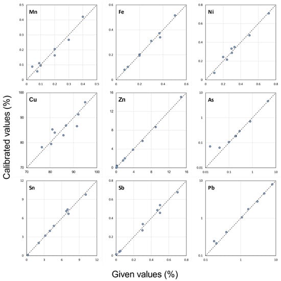
Figure A1.
Scatterplots of given versus calibrated values for the reference standards. The dashed black lines show the ideal 1:1 x-y line. As and Pb are shown with logarithmic axes.
Figure A1.
Scatterplots of given versus calibrated values for the reference standards. The dashed black lines show the ideal 1:1 x-y line. As and Pb are shown with logarithmic axes.
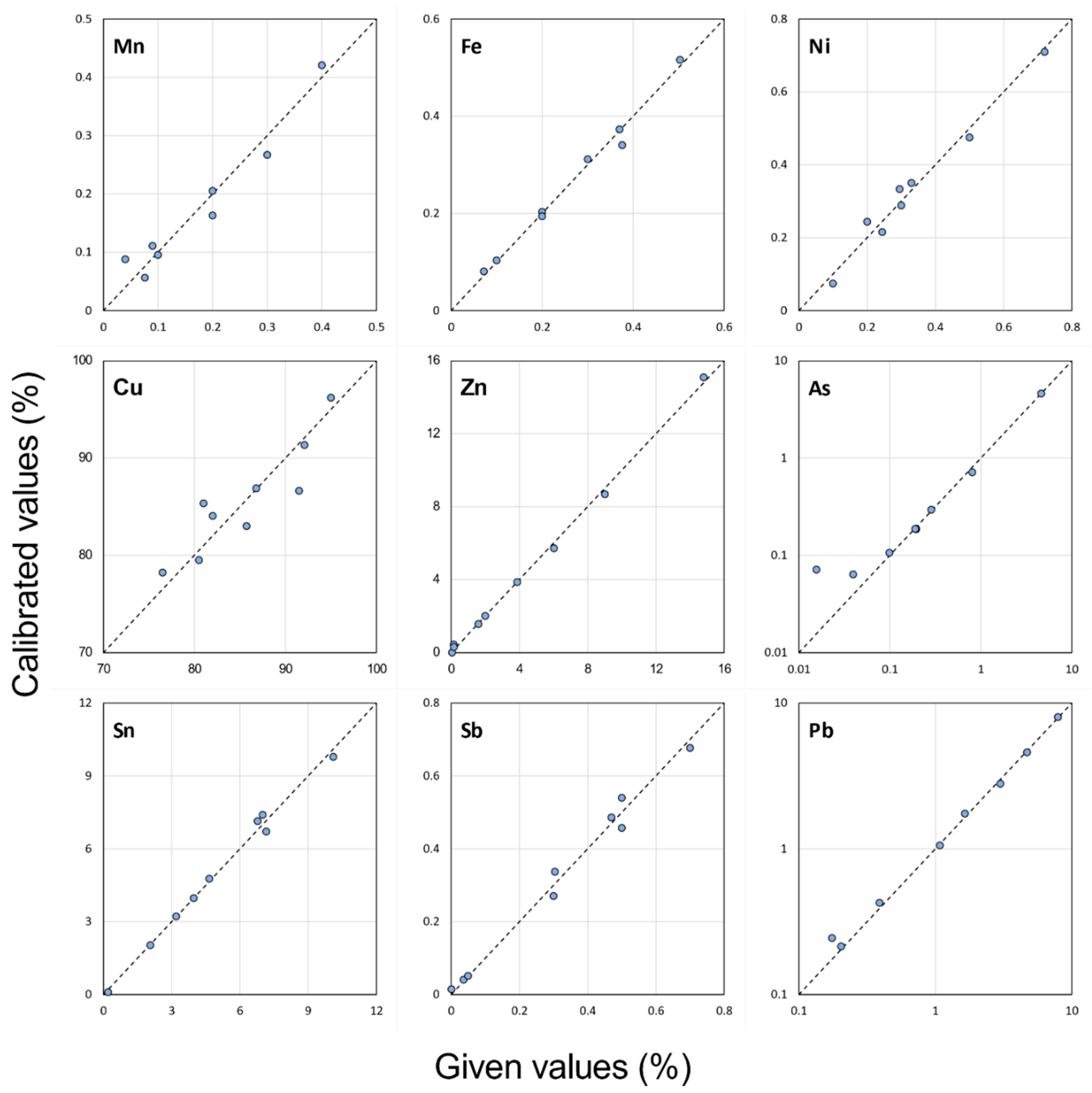
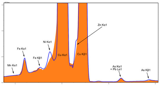
Figure A2.
Spectrum of a typical bronze piece, showing the Cu Kα peak overlap on Ni and the Cu Kβ overlap on Zn. The spectrum is shown in orange, guy and the fitted peaks (using Bruker’s Artax v.8.0 software) are shown as a blue line.
Figure A2.
Spectrum of a typical bronze piece, showing the Cu Kα peak overlap on Ni and the Cu Kβ overlap on Zn. The spectrum is shown in orange, guy and the fitted peaks (using Bruker’s Artax v.8.0 software) are shown as a blue line.

References
- Porter, S.T.; Huber, N.; Hoyer, C.; Floss, H. Portable and low-cost solutions to the imaging of Paleolithic art objects: A comparison of photogrammetry and reflectance transformation imaging. J. Archaeol. Sci. Rep. 2016, 10, 859–863. [Google Scholar] [CrossRef]
- Marín-Buzón, C.; Pérez-Romero, A.; López-Castro, J.L.; Jerbania, I.B.; Manzano-Agugliaro, F. Photogrammetry as a New Scientific Tool in Archaeology: Worldwide Research Trends. Sustainability 2021, 13, 5319. [Google Scholar] [CrossRef]
- Emmitt, J.J.; Mackrell, T.; Armstrong, J. Digital Modelling in Museum and Private Collections: A Case Study on Early Italic Armour. J. Comput. Appl. Archaeol. 2021, 4, 63–78. [Google Scholar] [CrossRef]
- Secci, M.; Demesticha, S.; Jimenez, C.; Papadopoulou, C.; Katsouri, I. A Living Shipwreck: An integrated three-dimensional analysis for the understanding of site formation processes in archaeological shipwreck sites. J. Archaeol. Sci. Rep. 2021, 35, 102731. [Google Scholar] [CrossRef]
- Charalambous, A.; Kassianidou, V.; Papassavas, G. A compositional study of Cypriot bronzes dating to the Early Iron Age using portable X-ray fluorescence spectrometry (pXRF). J. Archaeol. Sci. 2014, 46, 205–216. [Google Scholar] [CrossRef]
- Emmitt, J.; McAlister, A.; Armstrong, J. Pitfalls and Possibilities of Patinated Bronze: The Analysis of Pre-Roman Italian Armour Using pXRF. Minerals 2021, 11, 697. [Google Scholar] [CrossRef]
- Oudbashi, O.; Davami, P. Metallography and microstructure interpretation of some archaeological tin bronze vessels from Iran. Mater. Charact. 2014, 97, 74–82. [Google Scholar] [CrossRef]
- Colini, A.M. Veio. Scavi nell’area della città e della necropolis. Not. Degli Scavi 1919, 1919, 3–12. [Google Scholar]
- Ward-Perkins, J.B. Veii: The historical topography of the ancient city. Pap. Br. Sch. Rome 1961, 19, 1–124. [Google Scholar] [CrossRef] [Green Version]
- Delpino, F. Cronache Veientane. In Storia Delle Ricerche Archeologiche a Veio I. Dal XIV Alla Meta del XIX Secolo; Consiglio Nazionale delle Ricerche: Rome, Italy, 1985. [Google Scholar]
- Boitani, F. Veio-Casale del Fosso, tomba 1036. In Veio, Cerveteri e Vulci. Città d’Etruria a Confront; Moretti Sgubini, A.M., Ed.; Catalogo della Mostra: Rome, Italy, 2001; p. 112. [Google Scholar]
- Hencken, H. The Earliest European Bronze Helmets: Bronze Age and Early Iron Age; Peabody Museum Press: Cambridge, MA, USA, 1971. [Google Scholar]
- Iaia, C. Produzioni toreutiche della prima età del ferro in Italia centro-settentrionale. In Stili Decorativi, Circolazione, Significato; Biblioteca di Studi Etruschi: Rome, Italy, 2005. [Google Scholar]
- Iaia, C. Bronzesmiths and the Construction of Material Identity in Central Italy, (1000–700 BCE). In Crafting Connections: Production, Trade, and Identity in Pre-Roman Italy 900-400BCE; Armstrong, J., Cohen, S., Eds.; Routledge: London, UK, in press.
- Akoglu, K.G.; Kotoula, E.; Simon, S. Combined use of ultrasonic pulse velocity (UPV) testing and digital technologies: A model for long-term condition monitoring memorials in historic Grove Street Cemetery, New Haven. J. Cult. Herit. 2020, 41, 84–95. [Google Scholar] [CrossRef]
- Adamopoulos, E.; Rinaudo, F. Near-infrared modeling and enhanced visualization, as a novel approach for 3D decay mapping of stone sculptures. Archaeol. Anthropol. Sci. 2020, 12, 138. [Google Scholar] [CrossRef]
- Pfeuffer, C.; Rahrig, M.; Snethlage, R.; Drewello, R. 3D mapping as a tool for the planning of preservation measures on sculptures made of natural stone. Environ. Earth Sci. 2018, 77, 312. [Google Scholar] [CrossRef]
- Mozgai, V.; Bajnóczi, B.; May, Z.; Mráv, Z. Non-destructive handheld XRF study of archaeological composite silver objects—The case study of the late Roman Seuso Treasure. Archaeol. Anthropol. Sci. 2021, 13, 83. [Google Scholar] [CrossRef]
- Agisoft. Agisoft Metashape Professional, 1.5.3. 2019. Available online: http://www.agisoft.com/downloads/installer/ (accessed on 8 August 2021).
- Vitorino, T.; Casini, A.; Cucci, C.; Gebejesje, A.; Hiltunen, J.; Hauta-Kasari, M.; Picollo, M.; Stefani, L. Accuracy in Colour Reproduction: Using a ColorChecker Chart to Assess the Usefulness and Comparability of Data Acquired with Two Hyper-Spectral Systems. In Proceedings of the Computational Color Imaging, Cham, Germany, 24 March 2015; pp. 225–235. [Google Scholar]
- Marziali, S.; Dionisio, G. Photogrammetry and macro photography. The experience of the MUSINT II Project in the 3D digitizing process of small size archaeological artifacts. Stud. Digit. Herit. 2017, 1, 298–309. [Google Scholar] [CrossRef] [Green Version]
- Emmitt, J.; McAlister, A.; Bawden, N.; Armstrong, J. 3D and Assay Data Published in “XRF and 3D Modelling on a Composite Etruscan Helmet”; Zenodo: Geneva, Switzerland, 2021. [Google Scholar] [CrossRef]
- Karydas, A.G.; Anglos, D.; Harith, M.A. Mobile Micro-XRF and LIBS Spectrometers for Diagnostic Micro-Analysis of Ancient Metal Objects. In Metals and Museums in the Mediterranean: Protecting, Preserving and Interpreting; Argyropoulos, V., Ed.; Department of Conservation of Antiquities and Works of Art: Athens, Greece, 2008; pp. 141–177. [Google Scholar]
- Franzini, M.; Leoni, L.; Saitta, M. Determination of the X-ray mass absorption coefficient by measurement of the intensity of Ag Kα compton scattered radiation. X-Ray Spectrom. 1976, 5, 84–87. [Google Scholar] [CrossRef]
- Sullivan, C.B.; Kaszynski, A.A. PyVista: 3D plotting and mesh analysis through a streamlined interface for the Visualization Toolkit (VTK). J. Open Source Softw. 2019, 4, 1450. [Google Scholar] [CrossRef]
- Harman, J. Using decorrelation stretch to enhance rock art images. In Proceedings of the American Rock Art Research Association Annual Meeting, Sparks, NV, USA, 28 May 2005. [Google Scholar]
- Harman, J. Using DStretch for Rock Art Recording. Int. Newsl. Rock Art 2015, 72, 24–30. [Google Scholar]
- Schneider, C.A.; Rasband, W.S.; Eliceiri, K.W. NIH Image to ImageJ: 25 years of image analysis. Nat. Methods 2012, 9, 671–675. [Google Scholar] [CrossRef]
- Palomar-Vázquez, J.; Baselga Moreno, S.; Viñals Blasco, M.-J.; García-Sales, C.; SanchoEspinós, I. Application of a combination of digital image processing and 3D visualization of graffiti in heritage conservation. J. Archaeol. Sci. Rep. 2017, 12, 32–42. [Google Scholar] [CrossRef] [Green Version]
- Schreibman, S.; Papadopoulos, C. Textuality in 3D: Three-dimensional (re)constructions as digital scholarly editions. Int. J. Digit. Humanit. 2019, 1, 221–233. [Google Scholar] [CrossRef] [Green Version]
- Roxburgh, M.A.; Heeren, S.; Huisman, D.J.; Van Os, B.J.H. Non-Destructive Survey of Early Roman Copper-Alloy Brooches using Portable X-ray Fluorescence Spectrometry. Archaeometry 2019, 61, 55–69. [Google Scholar] [CrossRef]
- Zararsiz, A.; Zimmermann, T. The Missing Jigsaw Piece–pXRF Bulk Analysis of the Karaburun Dagger and Some General Considerations on Metalwork in Early Bronze Age Western Anatolia. Cedrus 2020, 8, 65–74. [Google Scholar] [CrossRef]


Publisher’s Note: MDPI stays neutral with regard to jurisdictional claims in published maps and institutional affiliations. |
© 2021 by the authors. Licensee MDPI, Basel, Switzerland. This article is an open access article distributed under the terms and conditions of the Creative Commons Attribution (CC BY) license (https://creativecommons.org/licenses/by/4.0/).