
A Forest Monitoring System for Tanzania


Abstract
:
1. Introduction
2. Methods
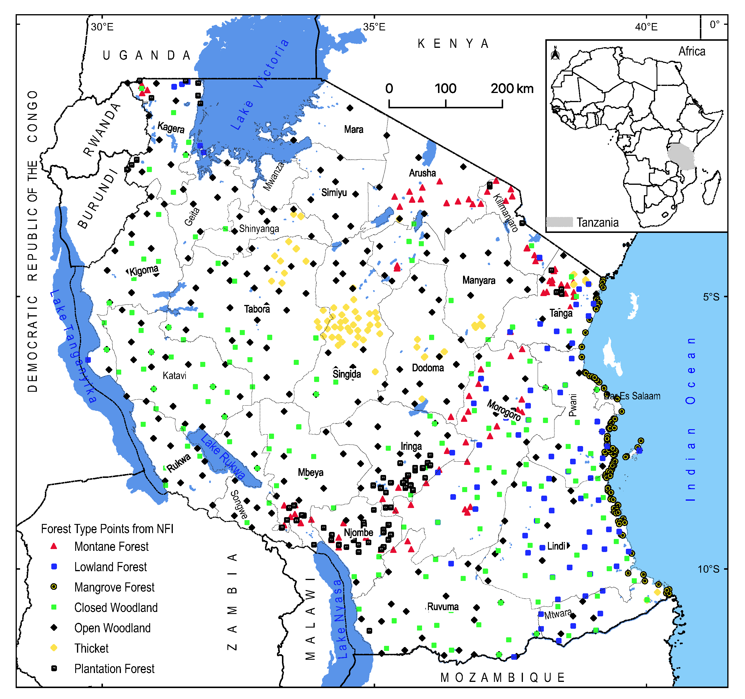
2.1. Study Area
2.2. Software and Data Processing
2.3. Landsat-8 Pre-Processing
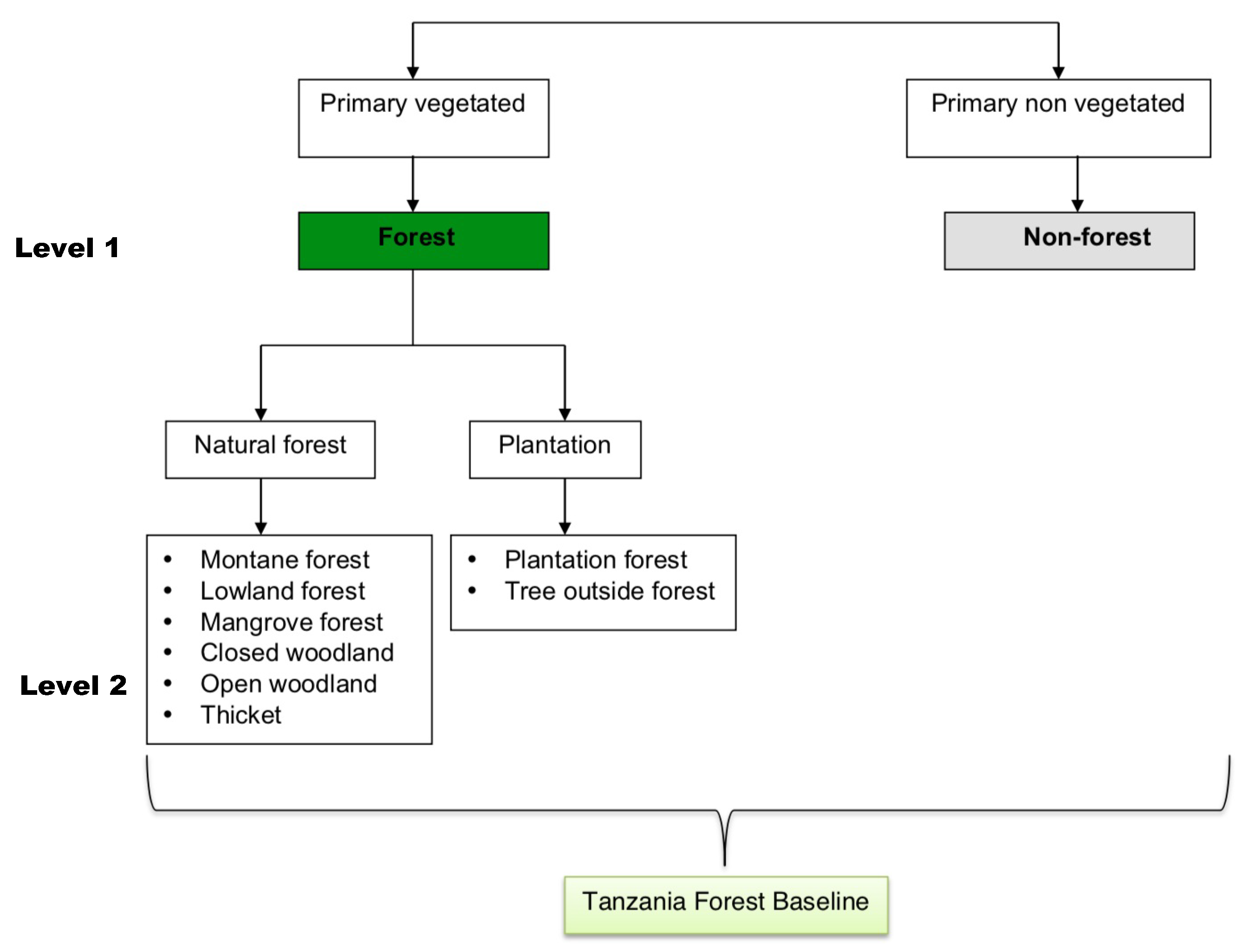
2.4. Classification Methodology
2.5. Forest/Non-Forest Classification
2.5.1. Defining Training Data
2.5.2. XGBoost Classifier
2.5.3. Optimising the XGBoost Parameters
2.5.4. Training the XGBoost Classifiers
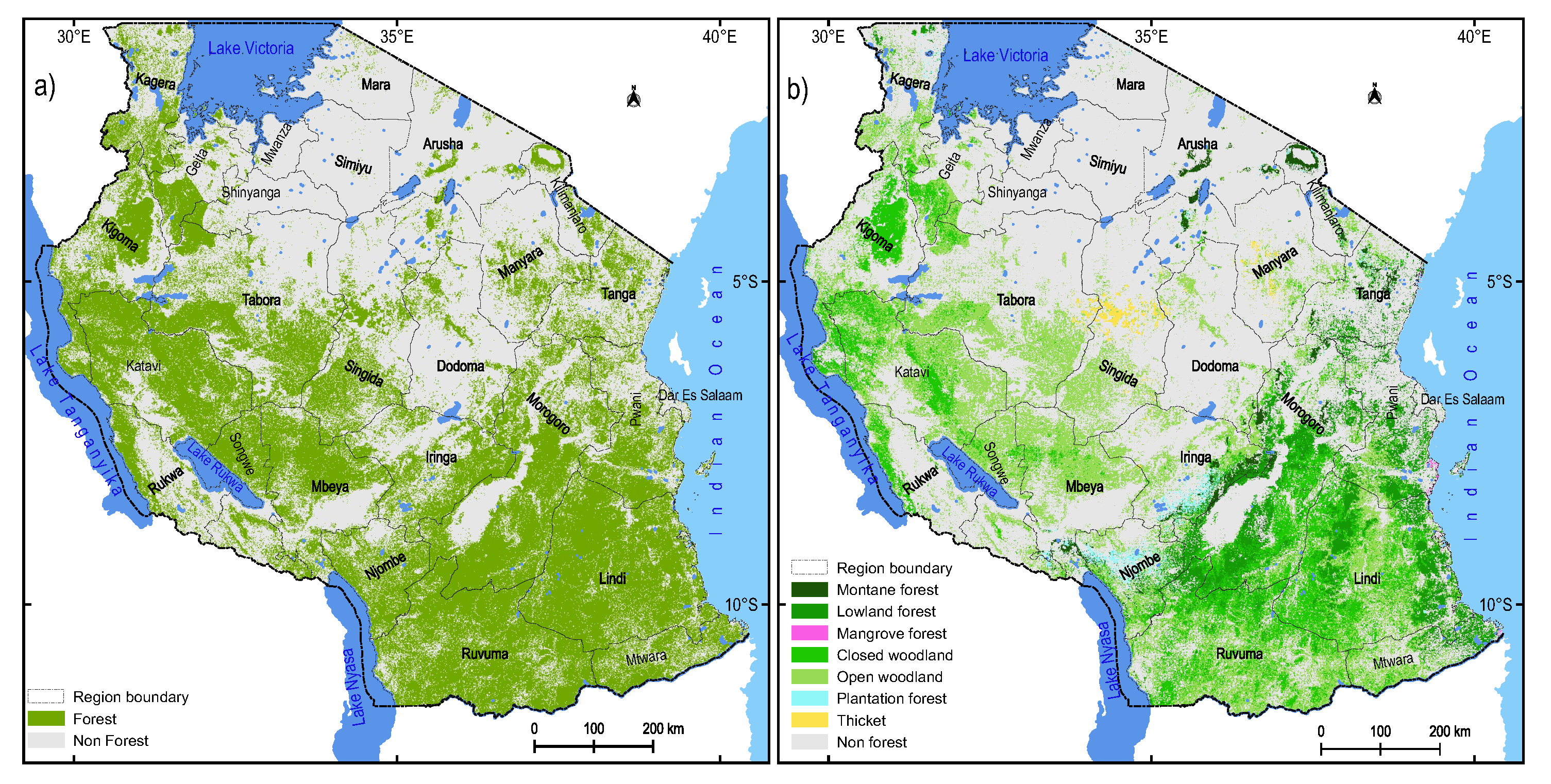
2.5.5. Creating the Final Forest Extent Map
2.5.6. Accuracy of the Forest Extent Map
2.6. Forest Type Classification
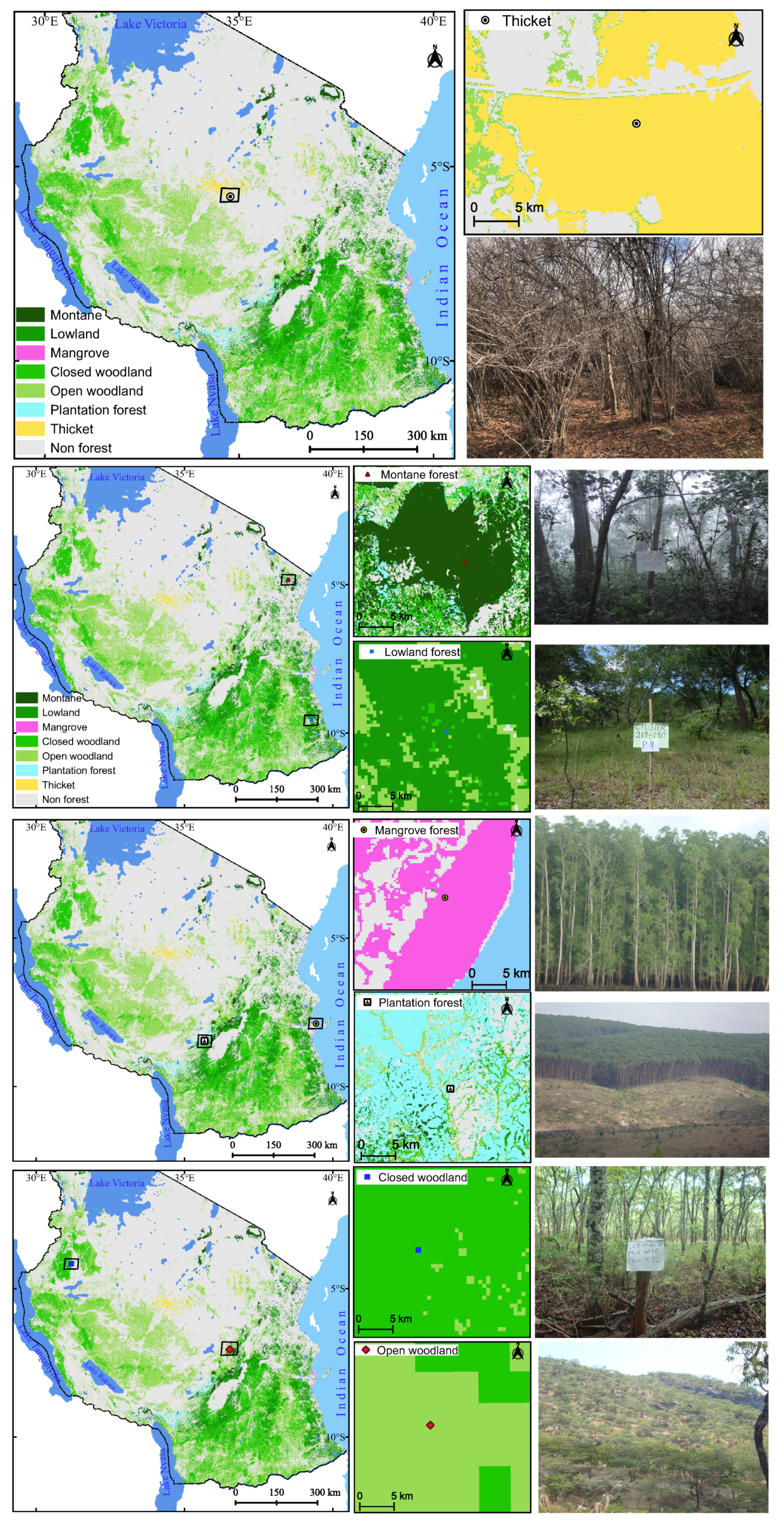
2.6.1. Forest Types Mask
2.6.2. Defining the Training Dataset
2.6.3. Training of the Classifiers
2.6.4. Final Forest Types Map
2.6.5. Accuracy of the Forest Types Map
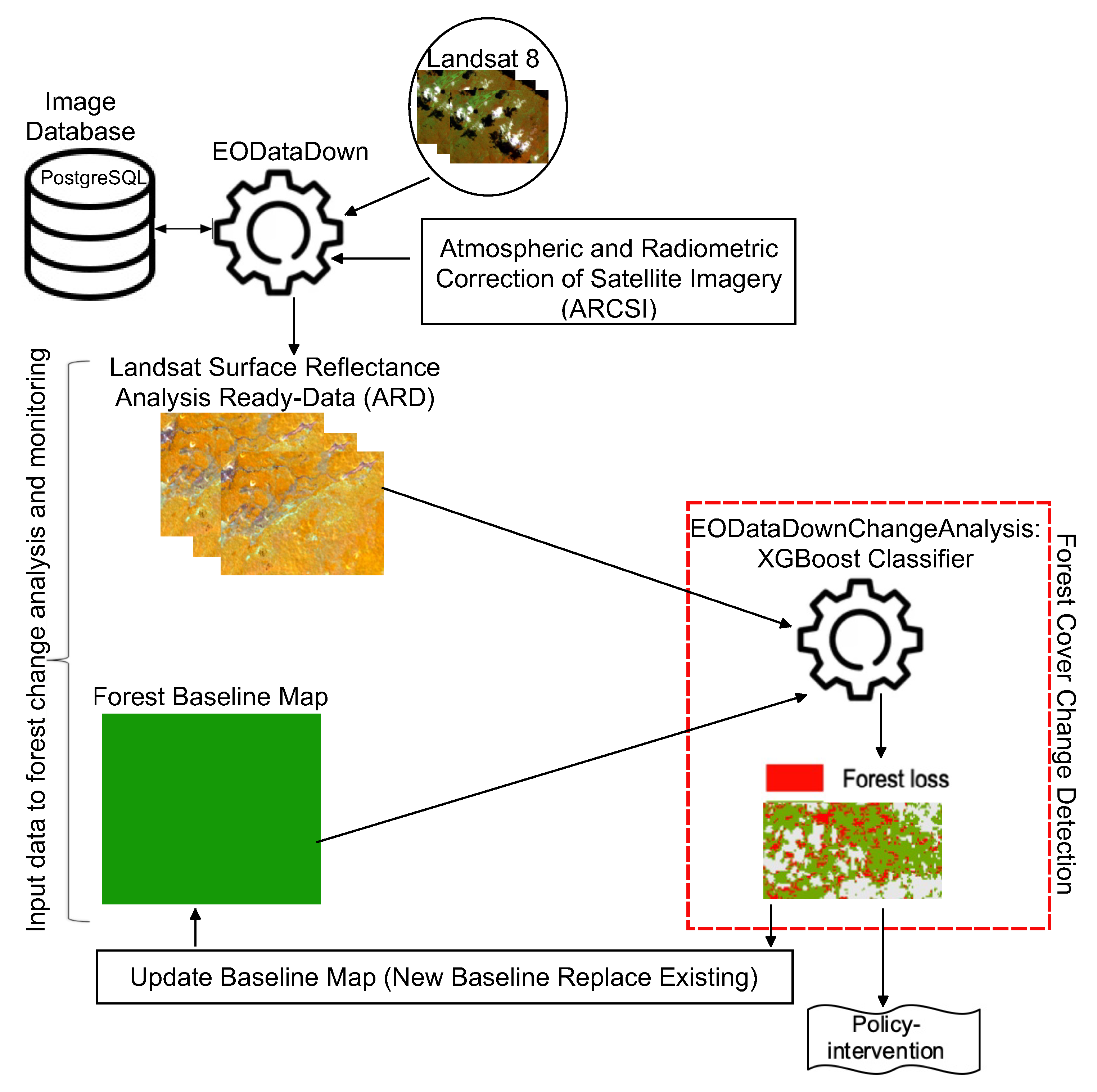
2.7. Forest Cover Change and Monitoring
2.7.1. System Architecture
2.7.2. Landsat 8 Imagery
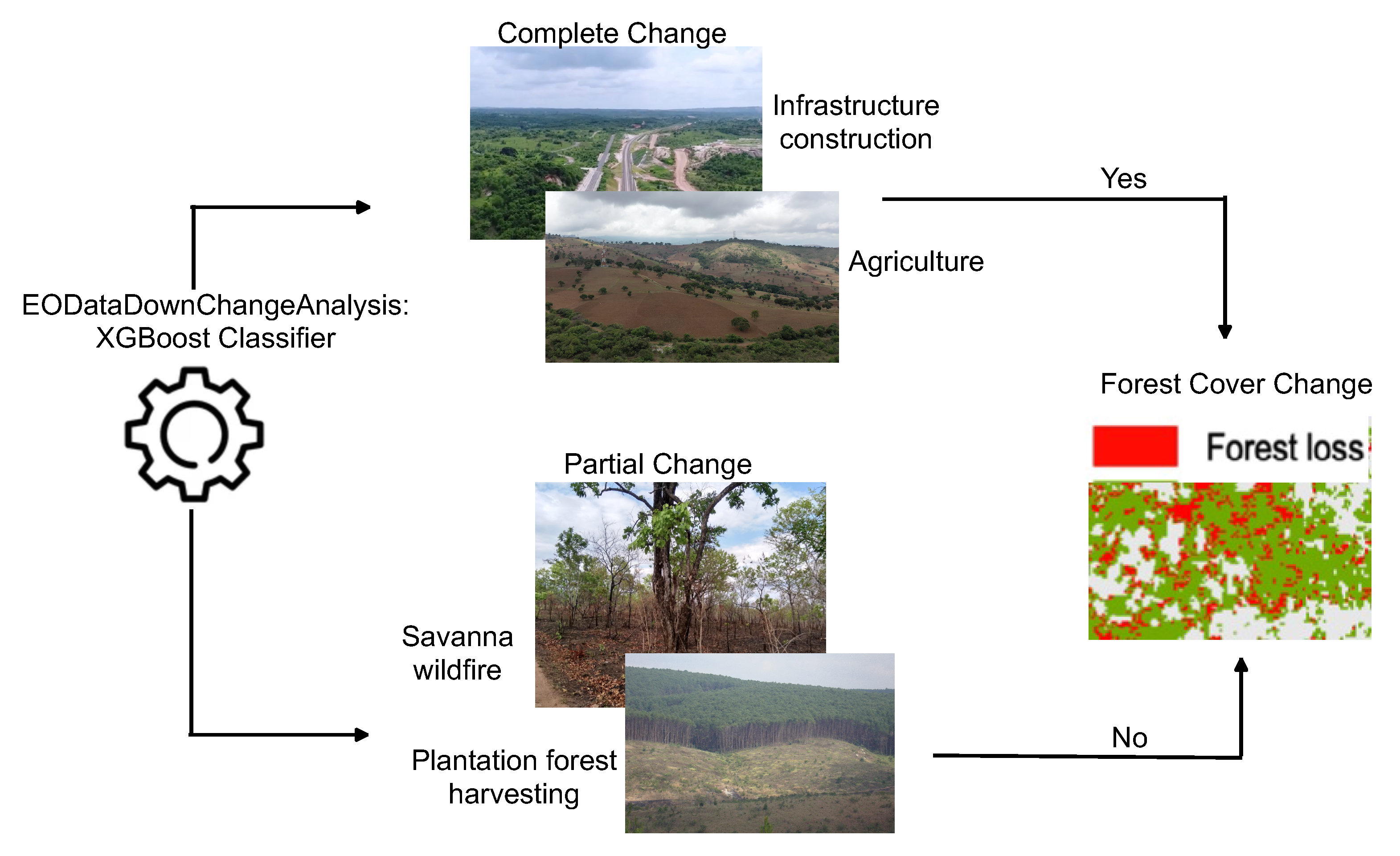
2.7.3. Forest Change Definition
2.7.4. Scene-Based Change Detection
2.7.5. Confirming Changes and Updating the Forest Baseline
2.7.6. Forest Change Accuracy Assessment
3. Results
3.1. Forest/Non-Forest Classification
3.1.1. Accuracy Assessment and Model Selection
3.1.2. Forest Area Estimates
3.2. Forest Types Classification
3.2.1. Accuracy Assessment
3.2.2. Forest Type Area Estimates
3.3. Estimated Forest Extent in Protected Areas
3.4. Forest Cover Change Results
3.4.1. Accuracy Assessment
3.4.2. Estimated Forest and Forest Type Change by Region
3.4.3. Estimated Forest Change in Protected Areas
3.4.4. Updating Earlier Forest Baseline
4. Discussion
4.1. Summary of Results
4.2. Forests and Forest Types Extent
4.3. Scene-Based Forest Change Detection
4.4. Forest Change Area Estimates
4.5. Forest Management Outlook
5. Conclusions
Author Contributions
Funding
Institutional Review Board Statement
Informed Consent Statement
Data Availability Statement
Acknowledgments
Conflicts of Interest
References
- Willis, K.J.; Bennett, K.D.; Burrough, S.L.; Macias-Fauria, M.; Tovar, C. Determining the response of African biota to climate change: Using the past to model the future. Philos. Trans. R. Soc. B Biol. Sci. 2013, 1625, 20120491. [Google Scholar] [CrossRef]
- Potapov, P.V.; Turubanova, S.A.; Hansen, M.C.; Adusei, B.; Broich, M.; Altstatt, A.; Mane, L.; Justice, C.O. Quantifying forest cover loss in Democratic Republic of the Congo, 2000–2010, with Landsat ETM+ data. Remote Sens. Environ. 2012, 122, 106–116. [Google Scholar] [CrossRef]
- Van Passel, J.; De Keersmaecker, W.; Somers, B. Monitoring woody cover dynamics in tropical dry forest ecosystems using sentinel-2 satellite imagery. Remote Sens. 2020, 12, 1276. [Google Scholar] [CrossRef] [Green Version]
- Bazzaz, F.A. Potential Impacts of Climate Change on Tropical Forest Ecosystems. In Tropical Forests in a Future Climate: Changes in Biological Diversity and Impact on the Global Carbon Cycle; Springer: Dordrecht, Netherlands, 1998; pp. 177–196. [Google Scholar]
- De Wasseige, C.; Flynn, J.; Louppe, D.; Hiol Hiol, F.; Mayaux, P. The Forests of the Congo Basin-State of the Forest 2013; Weyrich: Neufchâteau, Belgium, 2014; pp. 21–266. [Google Scholar]
- Fisher, R. Tropical forest monitoring, combining satellite and social data, to inform management and livelihood implications: Case studies from Indonesian West Timor. Int. J. Appl. Earth Obs. Geoinf. 2012, 16, 77–84. [Google Scholar] [CrossRef]
- Duveiller, G.; Defourny, P.; Desclée, B.; Mayaux, P. Deforestation in Central Africa: Estimates at regional, national and landscape levels by advanced processing of systematically-distributed Landsat extracts. Remote Sens. Environ. 2008, 112, 1969–1981. [Google Scholar] [CrossRef]
- Lambin, E.F.; Geist, H.J.; Lepers, E. Dynamics of land-use and land-cover change in tropical regions. Annu. Rev. Environ. Resour. 2003, 28, 205–241. [Google Scholar] [CrossRef] [Green Version]
- Mas, J.-F. Monitoring land-cover changes: A comparison of change detection techniques. Int. J. Remote Sens. 1999, 20, 139–152. [Google Scholar] [CrossRef]
- Godoy, F.L.; Tabor, K.; Burgess, N.D.; Mbilinyi, B.P.; Kashaigili, J.J.; Steininger, M.K. Deforestation and CO2 emissions in coastal Tanzania from 1990 to 2007. Environ. Conserv. 2012, 39, 62–71. [Google Scholar] [CrossRef] [Green Version]
- Malhi, Y.; Gardner, T.A.; Goldsmith, G.R.; Silman, M.R.; Zelazowski, P. Tropical forests in the Anthropocene. Annu. Rev. Environ. Resour. 2014, 39, 125–159. [Google Scholar] [CrossRef] [Green Version]
- Reiche, J.; Lucas, R.; Mitchell, A.L.; Verbesselt, J.; Hoekman, D.H.; Haarpaintner, J.; Herold, M.; Kellndorfer, J.M.; Rosenqvist, A.; Lehmann, E.A.; et al. Combining satellite data for better tropical forest monitoring. Annu. Rev. Environ. Resour. 2016, 6, 120–122. [Google Scholar] [CrossRef]
- Fuller, D.O. Tropical forest monitoring and remote sensing: A new era of transparency in forest governance? Singap. J. Trop. Geogr. 2006, 27, 15–29. [Google Scholar] [CrossRef]
- Hansen, M.C.; Potapov, P.V.; Moore, R.; Hancher, M.; Turubanova, S.A.; Tyukavina, A.; Thau, D.; Stehman, S.V.; Goetz, S.J.; Loveland, T.R.; et al. High-resolution global maps of 21st-century forest cover change. Science 2013, 342, 850–853. [Google Scholar] [CrossRef] [Green Version]
- Vesa, L.; Malimbwi, R.E.; Tomppo, E.; Zahabu, E.; Maliondo, S.; Chamuya, N.; Nsokko, E.; Otieno, J.; Dalsgaard, S. A National Forestry Resources Monitoring and Assessment of Tanzania (NAFORMA); Biophysical Survey. Field Manual; Ministry of Natural Resources & Tourism, Forestry and Beekeeping Division: Dar es Salaam, Tanzania, 2010; Available online: http://suaire.suanet.ac.tz/bitstream/handle/123456789/1287/Malimbwi17.pdf?sequence=1&isAllowed=y (accessed on 20 February 2021).
- Anderson, K.; Ryan, B.; Sonntag, W.; Kavvada, A.; Friedl, L. Earth observation in service of the 2030 Agenda for Sustainable Development. Geo-Spat. Inf. Sci. 2017, 20, 77–96. [Google Scholar] [CrossRef]
- Hardy, A.J.; Gamarra, J.G.P.; Cross, D.E.; Macklin, M.G.; Smith, M.W.; Kihonda, J.; Killeen, G.F.; Ling’ala, G.N.; Thomas, C.J. Habitat hydrology and geomorphology control the distribution of malaria vector larvae in rural Africa. PLoS ONE 2013, 12, e81931. [Google Scholar] [CrossRef] [PubMed] [Green Version]
- National Bureau of Statistics (NBS) [Tanzania]. National Environment Statistics Report; (NESR, 2017); NBS: Dar es Salaam, Tanzania, 2017; pp. 1–186.
- Burgess, N.; Hales, J.D.; Underwood, E.; Dinerstein, E.; Olson, D.; Itoua, I.; Schipper, J.; Ricketts, T.; Newman, K. Terrestrial Ecoregions of Africa and Madagascar: A Conservation Assessment; Island Press: Washington, DC, USA, 2004; pp. 1–150. [Google Scholar]
- MNRT. National Forest Resources Monitoring and Assessment (NAFORMA) Main Results; Tanzania Forest Services: Dar Es Salaam, Tanzania, 2015.
- John, E.; Bunting, P.; Hardy, A.; Roberts, O.; Giliba, R.; Silayo, D.S. Modelling the impact of climate change on Tanzanian forests. Divers. Distrib. 2020, 26, 1663–1686. [Google Scholar] [CrossRef]
- Bunting, P.; Clewley, D.; Lucas, R.M.; Gillingham, S. The Remote Sensing and GIS software library (RSGISLib). Comput. Geosci. 2014, 62, 216–226. [Google Scholar] [CrossRef]
- Bunting, P.; Gillingham, S. The KEA image file format. Comput. Geosci. 2013, 57, 54–58. [Google Scholar] [CrossRef]
- Chen, T.; Guestrin, C. XGBoost: A Scalable Tree Boosting System. In Proceedings of the 22nd ACM SIGKDD International Conference on Knowledge Discovery and Data Mining, San Francisco, CA, USA, 13–17 August 2016. [Google Scholar] [CrossRef] [Green Version]
- Bunting, P. Earth Observation Data Downloader (EODataDown). 2018. Available online: https://eodatadown.remotesensing.info (accessed on 14 January 2021).
- Bunting, P.; Clewley, D. Atmospheric and Radiometric Correction of Satellite Imagery (ARCSI). 2018. Available online: https://arcsi.remotesensing.info (accessed on 15 January 2021).
- Irons, J.R.; Dwyer, J.L.; Barsi, J.A. The next Landsat satellite: The Landsat data continuity mission. Remote Sens. Environ. 2012, 122, 11–21. [Google Scholar] [CrossRef] [Green Version]
- Mitchard, E.T.A.; Saatchi, S.S.; White, L.J.T.; Abernethy, K.A.; Jeffery, K.J.; Lewis, S.L.; Collins, M.; Lefsky, M.A.; Leal, M.E.; Woodhouse, I.H.; et al. Mapping tropical forest biomass with radar and spaceborne LiDAR in Lopé National Park, Gabon: Overcoming problems of high biomass and persistent cloud. Biogeosciences 2012, 9, 179–191. [Google Scholar] [CrossRef] [Green Version]
- Chavez, P.S., Jr. An improved dark-object subtraction technique for atmospheric scattering correction of multispectral data. Remote Sens. Environ. 1988, 24, 459–479. [Google Scholar] [CrossRef]
- Vermote, E.F.; Tanré, D.; Deuze, J.L.; Herman, M.; Morcette, J.J. Second simulation of the satellite signal in the solar spectrum, 6S: An overview. IEEE Trans. Geosci. Remote Sens. 1997, 35, 675–686. [Google Scholar] [CrossRef] [Green Version]
- Shepherd, J.D.; Dymond, J.R. Correcting satellite imagery for the variance of reflectance and illumination with topography. Remote Sens. Environ. 2003, 24, 3503–3514. [Google Scholar] [CrossRef]
- Bunting, P.; Rosenqvist, A.; Lucas, R.M.; Rebelo, L.M.; Hilarides, L.; Thomas, N.; Hardy, A.; Itoh, T.; Shimada, M.; Finlayson, C. The global mangrove watch—A new 2010 global baseline of mangrove extent. Remote Sens. 2018, 10, 1669. [Google Scholar] [CrossRef] [Green Version]
- Li, Y.; Li, C.; Li, M.; Liu, Z. Influence of variable selection and forest type on forest aboveground biomass estimation using machine learning algorithms. Forests 2019, 10, 1073. [Google Scholar] [CrossRef] [Green Version]
- Yu, L.; Gong, P. Google Earth as a virtual globe tool for Earth science applications at the global scale: Progress and perspectives. Int. J. Remote Sens. 2012, 33, 3966–3986. [Google Scholar] [CrossRef]
- Olofsson, P.; Foody, G.M.; Stehman, S.V.; Woodcock, C.E. Making better use of accuracy data in land change studies: Estimating accuracy and area and quantifying uncertainty using stratified estimation. Remote Sens. Environ. 2013, 129, 122–131. [Google Scholar] [CrossRef]
- Pontius, R.G., Jr.; Millones, M. Death to Kappa: Birth of quantity disagreement and allocation disagreement for accuracy assessment. Int. J. Remote Sens. 2011, 32, 4407–4429. [Google Scholar] [CrossRef]
- Schuster, C.; Förster, M.; Kleinschmit, B. Testing the red edge channel for improving land-use classifications based on high-resolution multi-spectral satellite data. Int. J. Remote Sens. 2012, 33, 5583–5599. [Google Scholar] [CrossRef]
- Boughorbel, S.; Jarray, F.; El-Anbari, M. Optimal classifier for imbalanced data using Matthews Correlation Coefficient metric. PLoS ONE 2017, 12, e0177678. [Google Scholar] [CrossRef]
- Hijmans, R.J.; Cameron, S.E.; Parra, J.L.; Jones, P.G.; Jarvis, A. Very high resolution interpolated climate surfaces for global land areas. Int. J. Climatol. J. R. Meteorol. Soc. 2005, 15, 1965–1978. [Google Scholar] [CrossRef]
- Reiche, J.; Mullissa, A.; Slagter, B.; Gou, Y.; Tsendbazar, N.-E.; Odongo-Braun, C.; Vollrath, A.; Weisse, M.J.; Stolle, F.; Pickens, A.; et al. Forest disturbance alerts for the Congo Basin using Sentinel-1. Environ. Res. Lett. 2021, 16, 024005. [Google Scholar] [CrossRef]
- García, M.L.; Caselles, V. Mapping burns and natural reforestation using Thematic Mapper data. Geocarto Int. 1991, 6, 31–37. [Google Scholar] [CrossRef]
- Chuvieco, E.; Martin, M.P.; Palacios, A. Assessment of different spectral indices in the red-near-infrared spectral domain for burned land discrimination. Int. J. Remote Sens. 2002, 23, 5103–5110. [Google Scholar] [CrossRef]
- Olofsson, P.; Arévalo, P.; Espejo, A.B.; Green, C.; Lindquist, E.; McRoberts, R.E.; Sanz, M.J. Mitigating the effects of omission errors on area and area change estimates. Remote Sens. Environ. 2020, 236, 111492. [Google Scholar] [CrossRef]
- Pitkänen, T.P.; Sirro, L.; Häme, L.; Häme, T.; Törmä, M.; Kangas, A. Errors related to the automatized satellite-based change detection of boreal forests in Finland. Int. J. Appl. Earth Obs. Geoinf. 2020, 86, 102011. [Google Scholar] [CrossRef]
- UNEP-WCMC. Protected Area Profile for United Republic of Tanzania from the World Database of Protected Areas. May 2021. Available online: http://www.protectedplanet.net/country/TZA (accessed on 25 May 2021).
- Hościło, A.; Lewandowska, A. Mapping forest type and tree species on a regional scale using multi-temporal Sentinel-2 data. Remote Sens. 2019, 11, 929. [Google Scholar] [CrossRef] [Green Version]
- Fjeldså, J. The impact of human forest disturbance on the endemic avifauna of the Udzungwa Mountains, Tanzania. Bird Conserv. Int. 1999, 9, 47–62. [Google Scholar] [CrossRef] [Green Version]
- Encalada, A.C.; Flecker, A.S.; Poff, N.L.; Suárez, E.; Herrera-R, G.A.; Ríos-Touma, B.; Jumani, S.; Larson, E.I.; Anderson, E.P. A global perspective on tropical montane rivers. Science 2019, 365, 1124–1129. [Google Scholar] [CrossRef]
- Mitchell, A.L.; Rosenqvist, A.; Mora, B. Current remote sensing approaches to monitoring forest degradation in support of countries measurement, reporting and verification (MRV) systems for REDD+. Carbon Balance Manag. 2017, 12, 1–22. [Google Scholar] [CrossRef] [Green Version]
- Rosa, I.; Rentsch, D.; Hopcraft, J.G.C. Evaluating forest protection strategies: A comparison of land-use systems to preventing forest loss in Tanzania. Carbon Balance Manag. 2018, 10, 4476. [Google Scholar] [CrossRef]
- Kimambo, N.E.; Naughton-Treves, L. The Role of woodlots in forest regeneration outside protected areas: Lessons from Tanzania. Forests 2019, 10, 621. [Google Scholar] [CrossRef] [Green Version]
- Suarez, D.R.; Rozendaal, D.M.A.; Sy, V.D.; Gibbs, D.A.; Harris, N.L.; Sexton, J.O.; Feng, M.; Channan, S.; Zahabu, E.; Silayo, D.S.; et al. Variation in aboveground biomass in forests and woodlands in Tanzania along gradients in environmental conditions and human use. Environ. Res. Lett. 2021, 16, 044014. [Google Scholar] [CrossRef]
- Verbesselt, J.; Hyndman, R.; Zeileis, A.; Culvenor, D. Phenological Change Detection While Accounting for Abrupt and Gradual Trends in Satellite Image Time Series. Remote Sens. Environ. 2010, 114, 2970–2980. [Google Scholar] [CrossRef] [Green Version]
- DeVries, B.; Verbesselt, J.; Kooistra, L.; Herold, M. Robust Monitoring of Small-Scale Forest Disturbances in a Tropical Montane Forest Using Landsat Time Series. Remote Sens. Environ. 2015, 161, 107–121. [Google Scholar] [CrossRef]
- Zhu, Z.; Woodcock, C.E. Continuous change detection and classification of land cover using all available Landsat data. Remote Sens. Environ. 2014, 144, 152–171. [Google Scholar] [CrossRef] [Green Version]
- Ghaderpour, E.; Vujadinovic, T. Change Detection within Remotely Sensed Satellite Image Time Series via Spectral Analysis. Remote Sens. 2020, 12, 4001. [Google Scholar] [CrossRef]
- Brooks, E.B.; Wynne, R.H.; Thomas, V.A.; Blinn, C.E.; Coulston, J.W. On-the-Fly Massively Multitemporal Change Detection Using Statistical Quality Control Charts and Landsat Data. IEEE Trans. Geosci. Remote Sens. 2014, 52, 3316–3332. [Google Scholar] [CrossRef]
- Awty-Carroll, K.; Bunting, P.; Hardy, A.; Bell, G. An evaluation and comparison of four dense time series change detection methods using simulated data. Remote Sens. 2019, 11, 2779. [Google Scholar] [CrossRef] [Green Version]
- Awty-Carroll, K.; Bunting, P.; Hardy, A.; Bell, G. Using Continuous Change Detection and Classification of Landsat Data to Investigate Long-Term Mangrove Dynamics in the Sundarbans Region. Remote Sens. 2019, 11, 2833. [Google Scholar] [CrossRef] [Green Version]
- Saxena, R.; Watson, L.T.; Wynne, R.H.; Brooks, E.B.; Thomas, V.A.; Zhiqiang, Y.; Kennedy, R.E. Towards a polyalgorithm for land use change detection. ISPRS J. Photogramm. Remote Sens. 2018, 144, 217–234. [Google Scholar] [CrossRef]
- Wu, L.; Li, Z.; Liu, X.; Zhu, L.; Tang, Y.; Zhang, B.; Xu, B.; Liu, M.; Meng, Y.; Liu, B. Multi-type forest change detection using BFAST and monthly landsat time series for monitoring spatiotemporal dynamics of forests in subtropical wetland. Remote Sens. 2020, 12, 341. [Google Scholar] [CrossRef] [Green Version]
- Neeff, T.; Piazza, M. How countries link forest monitoring into policy-making. For. Policy Econ. 2020, 118, 102248. [Google Scholar] [CrossRef]
- Galiatsatos, N.; Donoghue, D.N.; Watt, P.; Bholanath, P.; Pickering, J.; Hansen, M.C.; Mahmood, A.R. An assessment of global forest change datasets for national forest monitoring and reporting. Remote Sens. 2020, 12, 1790. [Google Scholar] [CrossRef]
- Chen, H.; Zeng, Z.; Wu, J.; Peng, L.; Lakshmi, V.; Yang, H.; Liu, J. Large Uncertainty on Forest Area Change in the Early 21st Century among Widely Used Global Land Cover Datasets. Remote Sens. 2020, 12, 3502. [Google Scholar] [CrossRef]
- Anande, D.M.; Luhunga, P.M. Assessment of Socio-Economic Impacts of the December 2011 Flood Event in Dar es Salaam, Tanzania. Atmos. Clim. Sci. 2019, 9, 421. [Google Scholar] [CrossRef] [Green Version]


| Predicted Combination | |||
|---|---|---|---|
| Value | Habitat Type Predicted | Yes = 1/No = 0 | Added Class |
| 2 | Montane forest | 1 | Lowland forest, plantation forest |
| Lowland forest | 0 | ||
| Mangrove forest | 0 | ||
| Plantation forest | 0 | ||
| Closed woodland | 0 | ||
| Open woodland | 0 | ||
| Thicket | 0 | ||
| 4 | Montane forest | 0 | |
| Lowland forest | 0 | ||
| Mangrove forest | 0 | ||
| Plantation forest | 0 | ||
| Closed woodland | 0 | ||
| Open woodland | 0 | ||
| Thicket | 1 | Open woodland, closed woodland | |
| 8 | Montane forest | 0 | |
| Lowland forest | 0 | ||
| Mangrove forest | 0 | ||
| Plantation forest | 1 | Montane, lowland forest | |
| Closed woodland | 0 | ||
| Open woodland | 0 | ||
| Thicket | 0 | ||
| 16 | Montane forest | 0 | |
| Lowland forest | 0 | ||
| Mangrove forest | 0 | ||
| Plantation forest | 0 | ||
| Closed woodland | 0 | ||
| Open woodland | 1 | Closed woodland, lowland forest | |
| Thicket | 0 | ||
| 32 | Montane forest | 0 | |
| Lowland forest | 0 | ||
| Mangrove forest | 0 | ||
| Plantation forest | 0 | ||
| Closed woodland | 1 | Open woodland, lowland forest | |
| Open woodland | 0 | ||
| Thicket | 0 | ||
| 64 | Montane forest | 0 | |
| Lowland forest | 1 | Montane forest, closed woodland | |
| Mangrove forest | 0 | ||
| Plantation forest | 0 | ||
| Closed woodland | 0 | ||
| Open woodland | 0 | ||
| Thicket | 0 | ||
| 128 | Montane forest | 0 | |
| Lowland forest | 0 | ||
| Mangrove forest | 1 | Lowland forest, closed woodland | |
| Plantation forest | 0 | ||
| Closed woodland | 0 | ||
| Open woodland | 0 | ||
| Thicket | 0 | ||
| Forest Type | Sample Polygons | Pixel Samples |
|---|---|---|
| Montane | 1272 | 7,638,017 |
| Lowland | 2053 | 19,192,926 |
| Mangrove | 1407 | 2,225,183 |
| Plantation | 794 | 2,118,903 |
| Closed Woodland | 3264 | 34,636,347 |
| Open Woodland | 11,070 | 165,439,923 |
| Thicket | 510 | 18,051,337 |
| Classification Model | |||||||
|---|---|---|---|---|---|---|---|
| Single-Scene (%) | Multi-Scene (%) | OA% | AD | QD | PC | TD | MCC |
| 30 | 30 | 68.46 ± 0.50 | 0.009 | 0.202 | 0.787 | 0.212 | 0.50 |
| 30 | 50 | 81.77 ± 0.50 | 0.029 | 0.123 | 0.847 | 0.152 | 0.67 |
| 30 | 80 | 88.17 ± 0.40 | 0.065 | 0.047 | 0.887 | 0.112 | 0.75 |
| 50 | 30 | 73.16 ± 0.50 | 0.016 | 0.181 | 0.802 | 0.197 | 0.56 |
| 50 | 50 | 88.11 ± 0.40 | 0.049 | 0.061 | 0.889 | 0.110 | 0.77 |
| 50 | 80 | 85.93 ± 0.40 | 0.039 | 0.080 | 0.879 | 0.120 | 0.72 |
| 80 | 30 | 80.84 ± 0.50 | 0.034 | 0.127 | 0.838 | 0.161 | 0.66 |
| 80 | 50 | 89.66 ± 0.40 | 0.100 | 0.003 | 0.896 | 0.103 | 0.78 |
| 80 | 80 | 81.24 ± 0.40 | 0.014 | 0.111 | 0.873 | 0.126 | 0.64 |
| Classification Model | |||||||||
|---|---|---|---|---|---|---|---|---|---|
| Single-Scene (%) | Multi-Scene (%) | Cover Type | UA% | PA% | F1 | P | R | C | O |
| 80 | 50 | Forest | 87.69 ± 0.70 | 87.86 ± 0.60 | 0.87 | 0.87 | 0.87 | 0.053 | 0.050 |
| Non-forest | 91.11 ± 0.50 | 90.98 ± 0.40 | 0.91 | 0.90 | 0.91 | 0.050 | 0.051 | ||
| 30 | 80 | Forest | 79.35 ± 0.90 | 91.59 ± 0.60 | 0.85 | 0.91 | 0.79 | 0.080 | 0.032 |
| Non-forest | 94.65 ± 0.40 | 86.20 ± 0.50 | 0.90 | 0.86 | 0.94 | 0.032 | 0.080 | ||
| 50 | 50 | Forest | 95.02 ± 0.40 | 80.43 ± 0.60 | 0.87 | 0.80 | 0.95 | 0.024 | 0.085 |
| Non-forest | 83.04 ± 0.70 | 95.79 ± 0.40 | 0.88 | 0.95 | 0.83 | 0.085 | 0.024 | ||
| Classification Model | ||||||
|---|---|---|---|---|---|---|
| Single-Scene (%) | Multi-Scenes (%) | Cover Type | Estimated Area (km) | Area (%) | NFI Area (km) | Area (%) |
| 30 | 30 | Forest | 756,686 | 84.87 | ||
| Non-forest | 134,913 | 15.13 | ||||
| 30 | 50 | Forest | 612,041 | 68.65 | ||
| Non-forest | 279,558 | 31.35 | ||||
| 30 | 80 | Forest | 321,124 | 36.02 | ||
| Non-forest | 570,476 | 63.98 | ||||
| 50 | 30 | Forest | 708,875 | 79.51 | ||
| Non-forest | 182,725 | 20.49 | ||||
| 50 | 50 | Forest | 521,238 | 58.46 | ||
| Non-forest | 370,361 | 41.54 | ||||
| 50 | 80 | Forest | 249,171 | 27.95 | ||
| Non-forest | 642,428 | 72.05 | ||||
| 80 | 30 | Forest | 614,830 | 68.96 | ||
| Non-forest | 276,770 | 31.04 | ||||
| 80 | 50 | Forest | 407,976 | 45.76 | 481,000 | 54.4 |
| Non-forest | 483,624 | 54.24 | 402,000 | 45.6 | ||
| 80 | 80 | Forest | 156,134 | 17.51 | ||
| Non-forest | 735,466 | 82.49 | ||||
| Rank | Region | Area (ha) | Area (%) |
|---|---|---|---|
| 1 | Lindi | 5,526,955 | 13.55 |
| 2 | Ruvuma | 5,059,867 | 12.40 |
| 3 | Morogoro | 4,295,711 | 10.53 |
| 4 | Katavi | 3,478,155 | 8.53 |
| 5 | Tabora | 3,054,801 | 7.49 |
| 6 | Mbeya | 2,163,746 | 5.30 |
| 7 | Kigoma | 1,988,670 | 4.87 |
| 8 | Iringa | 1,803,936 | 4.42 |
| 9 | Pwani | 1,739,369 | 4.26 |
| 10 | Singida | 1,689,458 | 4.14 |
| 11 | Njombe | 1,427,548 | 3.50 |
| 12 | Songwe | 1,220,258 | 2.99 |
| 13 | Mtwara | 1,203,790 | 2.95 |
| 14 | Kagera | 1,105,736 | 2.71 |
| 15 | Tanga | 951,165 | 2.33 |
| 16 | Manyara | 861,542 | 2.11 |
| 17 | Rukwa | 768,848 | 1.88 |
| 18 | Geita | 736,440 | 1.81 |
| 19 | Dodoma | 644,469 | 1.58 |
| 20 | Kilimanjaro | 377,028 | 0.92 |
| 21 | Arusha | 265,288 | 0.65 |
| 22 | Shinyanga | 177,709 | 0.44 |
| 23 | Mara | 92,345 | 0.23 |
| 24 | Mwanza | 89,022 | 0.22 |
| 25 | Dar Es Salaam | 43,970 | 0.11 |
| 26 | Simiyu | 31,773 | 0.08 |
| Forest Type | UA(%) | PA(%) | F1 | P | R | C | O |
|---|---|---|---|---|---|---|---|
| Montane forest | 88.53 ± 3.10 | 89.65 ± 2.80 | 0.89 | 0.89 | 0.88 | 0.002 | 0.003 |
| Lowland forest | 96.02 ± 0.90 | 88.55± 1.30 | 0.92 | 0.88 | 0.96 | 0.005 | 0.015 |
| Mangrove forest | 98.24 ± 0.34 | 100 ± 0.00 | 0.99 | 1 | 0.98 | 0.000 | 0.000 |
| Closed woodland | 72.35 ± 1.40 | 82.76 ± 1.10 | 0.77 | 0.83 | 0.72 | 0.067 | 0.049 |
| Open woodland | 89.73 ± 0.70 | 85.23 ± 0.60 | 0.87 | 0.85 | 0.89 | 0.057 | 0.068 |
| Plantation forest | 77.78 ± 5.5 | 90.32 ± 4.00 | 0.84 | 0.90 | 0.77 | 0.004 | 0.001 |
| Thicket | 89.60 ± 4.20 | 79.04 ± 4.00 | 0.84 | 0.79 | 0.89 | 0.001 | 0.003 |
| Overall accuracy (OA) | 85.22 ± 0.50 | ||||||
| Allocation disagreement (AD) | 0.11 | ||||||
| Quantity disagreement (QD) | 0.02 | ||||||
| Proportion correct (PC) | 0.86 | ||||||
| Total disagreement (TD) | 0.13 | ||||||
| Forest Types | Map Area (km) | Area(%) | NFI Area (km) | Area(%) |
|---|---|---|---|---|
| Montane forest | 9716 | 2.35 | 9953 | 2.03 |
| Lowland forest | 60,670 | 14.65 | 16,565 | 3.38 |
| Mangrove forest | 767 | 0.19 | 1581 | 0.32 |
| Closed woodland | 93,004 | 22.45 | 87,290 | 17.79 |
| Open woodland | 237,052 | 57.22 | 359,973 | 73.37 |
| Plantation forest | 6695 | 1.62 | 5545 | 1.13 |
| Thicket | 6368 | 1.54 | 9719 | 1.90 |
| Protected Area Category | ||||
|---|---|---|---|---|
| Cover | Forest Reserve | Area (%) | Wildlife Area | Area (%) |
| Forest | 6,911,300 | 17 | 11,339,583 | 28 |
| Forest Type (Area (ha)) | |||||||
|---|---|---|---|---|---|---|---|
| Category | Mo | Lo | Ma | CW | OW | PF | Th |
| Forest Reserve | 379,626 | 643,797 | 58,336 | 1,254,700 | 4,426,201 | 127,952 | 20,686 |
| Wildlife Area | 268,842 | 1,171,620 | - | 3,551,964 | 6,201,071 | - | 146,087 |
| Forest Cover Loss Area (ha) and Area (%) | ||||
|---|---|---|---|---|
| Class | This Study | % | Hansen et al. [14] | % |
| Forest Change | 157,204 | 0.39 | 142,773 | 0.36 |
| Class | Measure | This Study | Hansen et al. [14] |
|---|---|---|---|
| Change | Producer accuracy(%) | 96.13 ± 0.74 | 65.98 ± 2.04 |
| No-change | 92.74 ± 0.36 | 84.21 ± 0.33 | |
| Change | User accuracy(%) | 71.42 ± 1.52 | 34.25± 1.59 |
| No-change | 99.22 ± 0.15 | 95.20 ± 0.37 | |
| Change | Precision | 0.96 | 0.65 |
| No-change | 0.92 | 0.84 | |
| Change | Recall | 0.71 | 0.34 |
| No-change | 0.99 | 0.95 | |
| Change | F1-score | 0.82 | 0.45 |
| No-change | 0.96 | 0.89 | |
| Overall accuracy(%) | 93.28 ± 0.38 | 82.19 ± 0.59 |
| Area (ha), Year | |||
|---|---|---|---|
| Region | 2018 | 2019 | 2020 |
| Tabora | 211,412 | 31,587 | 5332 |
| Katavi | 120,629 | 23,171 | 2030 |
| Rukwa | 74,957 | 13,378 | 1360 |
| Mtwara | 30,431 | 12,633 | 2227 |
| Mbeya | 84,983 | 10,582 | 4185 |
| Lindi | 35,004 | 10,223 | 780 |
| Singida | 32,096 | 10,175 | 4268 |
| Kigoma | 76,750 | 8926 | 893 |
| Songwe | 72,716 | 7020 | 2945 |
| Iringa | 22,470 | 6033 | 664 |
| Ruvuma | 30,246 | 5991 | 638 |
| Morogoro | 16,674 | 5745 | 92 |
| Geita | 33,318 | 3630 | 338 |
| Pwani | 8120 | 1769 | 57 |
| Shinyanga | 10,449 | 1646 | 125 |
| Njombe | 5529 | 1384 | 111 |
| Dodoma | 5233 | 759 | 1054 |
| Kagera | 5823 | 411 | 57 |
| Mwanza | 3455 | 374 | 38 |
| Kilimanjaro | 27 | 28 | - |
| Tanga | 689 | 18 | 10 |
| Mara | 1453 | 18 | 10 |
| Simiyu | 91 | 10 | 6 |
| Manyara | 456 | 9 | 3 |
| Dar Es Salaam | 10 | 2 | - |
| Arusha | 19 | 1 | - |
| Forest Type Change (Area (ha))-2019 | |||||||
|---|---|---|---|---|---|---|---|
| Region | Mo | Lo | Ma | CW | OW | PF | Th |
| Tabora | - | - | - | 212 | 30,815 | - | 416 |
| Katavi | - | 2 | - | 687 | 21,256 | - | - |
| Rukwa | 8 | 2 | - | 1765 | 11,225 | - | - |
| Mbeya | 8 | 10 | - | 267 | 9860 | - | - |
| Singida | - | - | - | 40 | 7677 | - | 2441 |
| Kigoma | 11 | 20 | - | 1003 | 7432 | - | - |
| Songwe | 11 | 13 | - | 113 | 6689 | - | - |
| Iringa | 5 | 11 | 131 | 5382 | - | - | |
| Lindi | - | 3599 | 3 | 1221 | 4921 | - | - |
| Mtwara | - | 5891 | - | 869 | 4893 | - | - |
| Ruvuma | 7 | 154 | - | 843 | 4766 | - | - |
| Geita | - | 1 | - | 106 | 3519 | - | - |
| Morogoro | 13 | 1116 | - | 2582 | 1669 | - | - |
| Shinyanga | - | - | - | 13 | 1633 | - | - |
| Njombe | 9 | 151 | - | 53 | 709 | - | - |
| Dodoma | - | - | - | 83 | 630 | - | 16 |
| Pwani | - | 688 | - | 562 | 421 | - | - |
| Kagera | - | 1 | - | 18 | 390 | - | - |
| Mwanza | - | 81 | - | 48 | 239 | - | - |
| Kilimanjaro | - | - | - | 2 | 25 | - | - |
| Simiyu | - | - | - | - | 10 | - | - |
| Tanga | 3 | 7 | - | 5 | 8 | - | - |
| Manyara | - | - | - | - | 5 | - | 3 |
| Mara | - | - | - | 10 | 4 | - | - |
| Dar Es Salaam | - | - | - | - | 1 | - | - |
| Arusha | - | - | - | - | - | - | - |
| Area (ha), Year | |||
|---|---|---|---|
| Category | 2018 | 2019 | 2020 |
| Forest reserve | 126,925 | 24,869 | 3600 |
| Wildlife protected area | 72,153 | 13,587 | 2842 |
| Forest Cover Loss Area (km) | ||
|---|---|---|
| Class | This Study | Hansen et al. [14] |
| Forest change | 10,462.37 | 11,539.11 |
| Forest Area (km) for Earlier Baseline, Updated Baseline and Area (%) | ||||||
|---|---|---|---|---|---|---|
| Class | Earlier Baseline Extent | % | Estimate Forest Loss | % | Updated Baseline Extent | % |
| Forest | 407,976 | 45.76 | 10,462.37 | 2.56 | 397,514 | 43.20 |
Publisher’s Note: MDPI stays neutral with regard to jurisdictional claims in published maps and institutional affiliations. |
© 2021 by the authors. Licensee MDPI, Basel, Switzerland. This article is an open access article distributed under the terms and conditions of the Creative Commons Attribution (CC BY) license (https://creativecommons.org/licenses/by/4.0/).
Share and Cite
John, E.; Bunting, P.; Hardy, A.; Silayo, D.S.; Masunga, E. A Forest Monitoring System for Tanzania. Remote Sens. 2021, 13, 3081. https://doi.org/10.3390/rs13163081
John E, Bunting P, Hardy A, Silayo DS, Masunga E. A Forest Monitoring System for Tanzania. Remote Sensing. 2021; 13(16):3081. https://doi.org/10.3390/rs13163081
Chicago/Turabian StyleJohn, Elikana, Pete Bunting, Andy Hardy, Dos Santos Silayo, and Edgar Masunga. 2021. "A Forest Monitoring System for Tanzania" Remote Sensing 13, no. 16: 3081. https://doi.org/10.3390/rs13163081
APA StyleJohn, E., Bunting, P., Hardy, A., Silayo, D. S., & Masunga, E. (2021). A Forest Monitoring System for Tanzania. Remote Sensing, 13(16), 3081. https://doi.org/10.3390/rs13163081