Two-Stage Physical Economic Adjustable Capacity Evaluation Model of Electric Vehicles for Peak Shaving and Valley Filling Auxiliary Services

Abstract

A large number of renewable energy and EVs (electric vehicles) are connected to the grid, which brings huge peak shaving pressure to the power system. If we can make use of the flexible characteristics of EVs and effectively aggregate the adjustable resources of EVs to participate in power auxiliary services, this situation can be alleviated to a certain extent. In this paper, a two-stage physical and economic adjustable capacity evaluation model of EVs for peak shaving and valley filling ancillary services is constructed. The main steps are as follows: with the help of the deep learning ability of the AC (Actor-Critic) algorithm, the optimal physical charging scheme of EV fleet is determined to minimize the grid fluctuation under the travel constraints of private EVs, and the optimized charging power is transferred to the second stage. In the second stage, load aggregators encourage users to participate in ancillary services by setting subsidy prices. In this stage, the model constructs a user decision model based on a logistic function to describe the probability of users accepting dispatching instructions. With the goal of maximizing the revenue of load aggregators, the wolf colony algorithm is used to solve the optimal solution of the time-sharing subsidy level, and finally the economic adjustable capacity of the EV fleet considering the subjective decision of users is obtained.

1. Introduction

With the strong support of policies, EVs have achieved rapid development which is of positive significance to the greenhouse gas emission reduction and air pollution prevention and control in the transportation industry. However, with the continuous increase in the ownership of EVs, it also has a significant impact on power load forecasting and power system planning and operation [1,2,3]. The EV has strong adjustability, fast response speed and flexible adjustment mode [4,5,6,7] and its charging and discharging state can be directly controlled through the charging pile. After effective aggregation, it can provide multiple auxiliary services [8,9,10,11,12,13] and demand-side response [14] for the power system; at the same time, EV users can also obtain benefits by participating in the grid interaction [15,16], which is conducive to the benign development of the EV industry.

How to make use of the flexible characteristics of EVs and coordinate their charging and discharging time to weaken the impact of EV load on power grid operation and dispatching and achieve the effect of peak load reduction and valley filling has become one of the important problems in the current engineering field.

Some scholars have studied that it is possible to effectively transfer the charging time of EVs and pull up the low valley of power load at night by providing subsidies to EVs and guiding them to participate in the response of ancillary services [17], but a single aggregation goal is also very easy to generate new load peaks during the opening hours of ancillary services. Furthermore, some researches have begun to build a two-stage optimization model to realize multi-party optimization of the system by considering the grid operation objectives while aggregating the EV load or achieving collaborative optimization with renewable energy generation [18,19,20].

In the aspect of EV adjustable capacity evaluation, some studies have pointed out that the battery capacity, charging time, charging and discharging power [16,21] and the upper/lower limit of SOC [22] (state of charge) accepted by users are the important constraints of EV adjustable capacity evaluation.

In the construction of an EV scheduling model, most of the research focuses on the travel characteristics of EV users [23]. These models usually assume that users only need to set the time when the EV enters and leaves the network [24,25]. They think that as long as the controllable range of SOC meets the conditions, then the EV can be scheduled from the time when it enters the network to the time when it leaves. However, it should be noted that different from the traditional energy storage equipment, EVs, as a kind of high-quality controllable resources [26], are accompanied by the uncertainty of user decision-making. From this point of view, the current research lacks the subjective analysis of the EV users’ acceptance of scheduling. Due to the difference in users’ travel characteristics, the acceptance of the same dispatching instructions will be different [27], which will directly affect the final adjustable capacity.

Based on the research status, we constructed a two-stage physical and economic adjustable capacity evaluation model of EVs for participating in the ancillary services market.

The model is divided into two stages to evaluate its response ability to participate in ancillary services. (1) In the first stage, the travel data and charging load data of EVs are obtained. Under the condition of meeting the travel power demand of EVs, the best physical charging scheme of the EV fleet with the objective function of smooth grid fluctuation is determined by means of the in-depth learning ability of AC algorithm, and the optimized charging power is transferred to the second stage. (2) In the second stage, the load aggregator encourages users to participate in auxiliary services by setting subsidy price. In this stage, the user decision-making model based on logistic function is established to describe the probability of users accepting dispatching instructions, and the wolf colony algorithm is used to solve the optimal solution of the time-sharing subsidy level with the goal of maximizing the revenue of the load aggregator, Finally, the economic adjustable capacity of the EV fleet considering the subjective decision of users is obtained, which makes the evaluation results closer to the actual situation. Figure 1 is the logical framework of this paper.

2. First Stage: Physical Adjustable Capacity Assessment

According to the characteristics of automobile travel, EVs can be divided into four types: taxi, bus, private car and official car. Due to the profit-making nature of buses and taxis, in the operation time, when the SOC is low, most car owners choose the fast charging mode to charge immediately. In addition, the ability of buses and taxis to participate in auxiliary services is greatly affected by the actual scheduling situation. However, when the buses and taxis park at the station at night and the start and end time is extremely stable, it can be directly issued to the station to guide the charging time to transfer to the low load period, so the scheduling difficulty is relatively low. Most owners of private EVs will charge them immediately after they go home at night, which coincides with the peak height of electricity consumption in the evening [27]. According to statistics, except for buses and taxis, EVs are in parking state for more than 90% of the time in use. In addition, whether private EVs participate in dispatching or not requires each owner to make an independent decision, and the degree of user participation is strongly correlated with economic incentives. Therefore, theoretically, there is a large space for adjusting the charging time of private EVs. Business vehicles account for a small proportion, and the number of trips and travel time are stochastic, and most of the time they are in parking state, but the process of participating in response is similar to that of private cars. Therefore, it is of great practical significance to study how to guide private car users to participate in auxiliary services with appropriate economic incentives. Therefore, private cars are classified as the research object of this paper.

2.1. Travel Status Description of Private EVs

The travel activities of private cars are relatively clear and fixed, and the length of travel chain during working days is mostly three links (Home-Workplace-Home) [28]. In order to simplify the model, considering that private EVs are only used for commuting on and off duty on working days, a travel cycle is divided into four periods according to its travel law. g(t) is used to represent the state of EV connected to the power grid at time t, where:

$$g\left(t\right)=\{\begin{array}{c}0, \mathrm{Indicates} \mathrm{that} \mathrm{EV} \mathrm{is} \mathrm{off} \mathrm{grid}\\ 1, \mathrm{Indicates} \mathrm{that} \mathrm{EV} \mathrm{is} \mathrm{on} \mathrm{grid}\end{array}$$

(1)

The operation status of EVs in each period is described as follows:

• In the period ΔT₁: at the beginning of the travel cycle, the EV leaves the grid at full charge, and the battery is in the state of discharge, g(t) = 0;
• In the period ΔT₂: during the period from arriving at the work place in the morning to leaving the company after work, the vehicle is in the parking state and connected to the power grid. During the period, the vehicle is in the state of charging (discharge to the power grid is not considered) or idle state. The electric quantity needs to ensure the travel capacity required in the next period, g(t) = 1;
• In the period ΔT₃: at the time of driving home from work in the evening, EV is off the grid and the battery is in discharge state, g(t) = 0;
• In the period ΔT₄: during the period from returning home in the evening to going to work the next day, the vehicle is in the state of charging (the same as not considering discharging to the power grid) or idle state. Considering the sufficient charging time at night, it is necessary to ensure that the battery is fully charged in this period, g(t) = 1.

Generally speaking, EVs will not sacrifice the established travel routine in exchange for the benefits of participating in demand-side response. Therefore, this paper only studies the potential and capacity of EVs in the on-grid state, namely ΔT₂ and ΔT₄, without affecting users’ travel routine.

In addition, in the research of EV charging demand, most scholars at home and abroad analyze and describe the travel characteristics of EVs based on the travel data of fuel vehicles. Among them, some literatures point out that the commuting attributes of private EVs are obvious and have strong regularity. By analyzing the travel characteristics of private EVs, it is pointed out that the daily mileage is approximately logarithmic distribution [29], the first driving time conforms to normal distribution and the end travel time accords with Poisson distribution [22]. This paper will also build a private EV travel model based on the above research.

2.2. The Best Physical Charging Scheme for EVs Participating in Ancillary Services

Firstly, the model basis and assumptions are described:

• Based on EVi (i = 1, 2, …, N) of EV fleet in the case of ΔTi2 and ΔTi4 target periods as an example, let [tiin, tiout] denote the on-grid period, and tiin and tiout are respectively the time when the vehicle enters and leaves the grid (but does not represent the time when the vehicle i starts charging and finishes charging).
• The initial state of EVi connected to the power grid is recorded as SOCiin. In order to avoid excessive battery discharge, users will set a SOCimin value subjectively, and charge the EV when SOC is lower than SOCimin, and the user also hopes that the SOC of the battery is not lower than SOCimin as far as possible after the next journey.
• In the case of sufficient parking time, the user expects the EV charging to 100% by default [30]; however, considering the user’s psychology, if it is known that reducing part of the charging power can obtain economic subsidy, then under the incentive of subsidy, the user is willing to give up the requirement of off-grid full charge and set a relatively satisfactory expected rate of charge SOCiexc, SOCiexc ∈ [SOCiin, SOCmax]. That is to say, as long as the charging rate can reach SOCiexc when the user is off-grid, it will not affect the user’s enthusiasm for participating in the auxiliary service.

Based on literature research [31,32], the charging load transfer interval of EV_i participating in ancillary services under charging mode is given, as shown in Figure 2.

In this paper, the charging process is an unsteady power mode. When EV_i is fully charged to SOC_max in parking state, it will turn into idle state. The BC segment represents the constraint of compulsory charging to meet the travel demand; that is, if the EV is not charged at point B from the beginning of entering the network, even if the maximum rated power is used for charging before leaving the network, the SOC lower bound of off-grid SOC cannot be reached, so point B is the latest charging time for EVs. The latest charging time $t_{sj}^i$ and linear BC can be expressed as:

$$t_{{}_{sj}}^i=t_{{}_{out}}^i-\frac{\left({\underset{\_}{SOC}}^i-SO{C}_{in}^i\right)C_i}{p_{rated}^i\eta }$$

(2)

$$y=\frac{p_{rated}^i\eta }{C_i}(t-t_{out}^i)+SO{C}_{exc}^i$$

(3)

where $p_{rated}^i$ is the rated charging power of EV_i, which is considered as a constant value, and C_i is the battery capacity of EV_i, η is charging efficiency. When EVs participate in peak shaving auxiliary service, it is necessary to sacrifice off-grid SOC to expand the response capacity and further reduce the charging load during this period; at this time, there is ${\underset{\_}{SOC}}^i\le SO{C}^i{}_{out}\le SO{C}_{max}$.

EV_i is connected to the power grid at the time of $t_{in}^i$, and the charging pile obtains the charging information of EVs and the travel information of users. Taking minimizing the load fluctuation of the power grid as the objective function, the optimal charging scheme of the EV fleet is obtained according to in-grid time, off-grid time, SOC lower bound SOC and the latest charging time $t_{sj}^i$. The EVs participating in the regulation complete the charging in this period according to the charging instructions issued by the charging pile.

(1)

Objective function

$$min\frac{{\displaystyle \sum _{t=1}^{24}{\left(Q_{grid,t}+{\displaystyle \sum _{i=1}^N{\overline{p}}_t^i}-Q_{\mathrm{avg}}\right)}^2}}{Q_{\mathrm{avg}}^2}$$

(4)

where $Q_{grid,t}$ is the grid operation load at time t; ${\overline{p}}_t^i$ denotes the charging power of EV I at time t according to the best charging scheme; $Q_{\mathrm{avg}}$ is the average load of the grid in one day when the EV fleet is charged according to the best charging scheme.

(2)

Constraints

• Charging power constraint:

  $$0\le {\overline{p}}_t^i\le p_{rated}^i$$

  (5)
• Charging time constraint:

  $$t_{in}^i\le t\le t_{out}^i$$

  (6)
• SOC lower bound at off-grid time:

  $$SO{C}_{\min }^i+\frac{d^i{w}^i}{C^i}\le SO{C}_{out}^i\le 100\%$$

  (7)

  where Cⁱ is the battery capacity, dⁱ is the estimated mileage for the next journey and wⁱ is the EV power consumption per kilometer.
• If the charging scheme issued for EVs after entering to grid is not charging this time, it is necessary to ensure that the SOC at the end of the next journey is not less than $SO{C}_{\min }^i$:

  $$SO{C}_{\mathrm{in}}^i-\frac{d^i{w}^i}{C^i}\ge SO{C}_{\min }^i$$

  (8)

  Considering the abundant charging time of EVs at night and that the main purpose of charging at night is to meet the demand of grid valley filling, EVs should be charged as much as possible at night. In this paper, it is set that the off-grid SOC of EV should reach 100% after charging at night.

3. Evaluation of Economic Adjustable Capacity of EV Considering User Decision

Load aggregators aggregate EV fleets, issue instructions through EVA (distributed database and application platform of EV) interface, and users can obtain charging price information and supply and demand information through wireless terminals (smart phones, iPad, etc.).

3.1. EV User Decision Model Based on Logistic Function

Some studies think that EVs can be scheduled when connected to the power grid [33], but in reality, EV users have their own subjective will, and whether they accept EVA scheduling is affected by many factors. In view of the one-time decision-making of users, the final charging mode depends on the initial one-time decision-making of users in the process from EV access to the grid to leaving the grid. This paper mainly considers that when the user is faced with dispatching instructions, it will mainly evaluate them from two aspects—the subsidy level obtained by participating in the response and the difference of electricity perceived by the user in the two cases of participating and not participating in the response—so as to make the response decision. Therefore, this paper mainly studies the impact of the above two factors on user decision-making. Based on the logistic function, the problem is transformed into the problem of vehicle owners’ choice between accepting and not accepting scheduling instructions.

$$x_i={\alpha }_i+{\beta }_1\Delta SO{C}_i+{\beta }_2{u}_i+e$$

(9)

Among them, ΔSOC_i refers to the deviation of SOC from the expected SOC at the off-grid time.

$$\Delta SO{C}_i=\min \{SO{C}_{out}^i-SO{C}_{exc}^i,0\}$$

(10)

u_i represents the subsidy received by EV users through participating in the response:

(1)

When the response period is valley filling period:

$$u^i={\displaystyle \sum _{\begin{array}{l}t\in [t_{in}^i,t_{out}^i]\\ {\overline{p}}_t^i>p_t^i\end{array}}{s}_t({\overline{p}}_t^i-p_t^i})\Delta t$$

(11)

(2)

When the response period is peak shaving period:

$$u^i={\displaystyle \sum _{\begin{array}{l}t\in [t_{in}^i,t_{out}^i]\\ p_t^i\ge {\overline{p}}_t^i\end{array}}{s}_t(p_t^i-{\overline{p}}_t^i})\Delta t$$

(12)

where ${\overline{p}}_t^i$ is the charging power distributed to EV i at time t; $p_t^i$ is the reference charging power of EV at time t. x_i can be transformed into probability by a logistic function.

$$P_i(\mathrm{X}=1)=\mathrm{F}(x_i)=\frac{1}{1+e^{-x_i}}$$

(13)

$$P_i(\mathrm{X}=0)=1-P_i(\mathrm{X}=1)=\frac{1}{1+e^{x_i}}$$

(14)

The unit of subsidy level S_t is CNY/kWh; α is the benchmark probability coefficient; β₁, β₂ are variable coefficients (β₁ > 0, β₂ > 0); E is the error of random variables, in which the coefficients of each variable need to be obtained through investigation and fitting based on statistical data.

$$P_{orig,t}^i=\{\begin{array}{l}{p}_{rated}^i,t\in [t_{in}^i,t_{end}^i]\\ 0,t\notin [t_{in}^i,t_{end}^i]\end{array}$$

(15)

$$t_{{}_{end}}^i=\min \{t_{{}_{in}}^i+\frac{\left(SO{C}_{\max }-SO{C}_{in}^i\right)C_i}{p_{rated}^i\eta },t_{out}^i\}$$

(16)

where $p_{rated}^i$ is the rated charging power of EV_i.

In the background of this paper, the load aggregator sets the subsidy level S_t at each time according to the clearing price level of the ancillary service market in the target period, and then calculates the revenue and cost of EVs according to the SOC at the time when EV_i enters the grid and the user’s off-grid time and the lower bound of SOC at off-grid time; after it is distributed to users, users combine u_i and ΔSOC_i makes decisions. Therefore, from the perspective of user decision-making, ΔSOC_i in the physical scheduling scheme is a certain quantity, then Formula (2) is transformed after the fixed value part is merged:

$$a_i={\alpha }_i+{\beta }_1\Delta SO{C}_i$$

(17)

$$P_i(\mathrm{X}=1)=\frac{1}{1+e^{-(a_i+{\beta }_2{u}_i+e)}}$$

(18)

EVA can affect the user’s response revenue u by changing the subsidy s_t, thus affecting the probability of user participating in the response. As shown in Figure 3 below:

3.2. Analysis of Adjustable Capacity Considering User Decision

Under the mode of load aggregator, the load aggregator participates in the auxiliary service market on behalf of EV users in the superior market with the goal of maximizing the expected profit, and the decision variable $s=\left[s_1,s_2,s_3,\dots ,s_{24}\right]$ is the subsidy level for EVs at all times. The objective function is as follows.

$$\max f={\displaystyle \sum _{i=1}^N[{\displaystyle \sum _{t=1}^{24}{\rho }_{t,m}^i}}\cdot P(\mathrm{X}=1)]$$

(19)

(1)

When the response period is valley filling period:

$${\rho }_{t,m}^i={\displaystyle \sum _{\begin{array}{l}t\in [t_{in}^i,t_{out}^i]\\ {\overline{p}}_t^i\le {p^{\prime }}_t^i\end{array}}(p_{market,t}-s_t)({p^{\prime }}_t^i-p_t^i})\Delta t$$

(20)

(2)

When the response period is peak shaving period:

$${\rho }_{t,m}^i={\displaystyle \sum _{\begin{array}{l}t\in [t_{in}^i,t_{out}^i]\\ p_t^i\ge {p^{\prime }}_t^i\end{array}}(p_{market,t}-s_t)(p_t^i-}{p^{\prime }}_t^i)\Delta t$$

(21)

s.j.

$$0\le s_t^i\le pric{e}_{market,t}$$

(22)

where N is the number of EVs; ${p^{\prime }}_t^i$ represents the actual charging power of EV I at time t; $p_t^i$ is the reference charging power of EV at time t; ${\rho }_{t,m}^i$ represents the revenue of the load aggregator at time t by stimulating EVs to participate in the response; price_market,t is the forecast clearing price level (unit: KWH) of the ancillary services market period at time t.

The economic adjustable capacity of EV cluster considering user decision at time t is as follows:

$$Q_{adj,t}=\{\begin{array}{l}{\displaystyle \sum _{i=1}^N\max \{{p^{\prime }}_t^i-p_t^i,0\}},t\in {\mathrm{T}}_{valley}\\ {\displaystyle \sum _{i=1}^N\max \{p_t^i-{p^{\prime }}_t^i,0\},t\in {\mathrm{T}}_{peak}}\end{array}$$

(23)

where ${p^{\prime }}_t^i$ and ${\overline{p}}_t^i$ represent the actual charging power of EV_i participating in the response and the reference charging power of EV_i not participating in the auxiliary service response at time t; ${\mathrm{T}}_{valley}$ and ${\mathrm{T}}_{peak}$ are valley filling and peak shaving, respectively.

4. Solution Method

4.1. AC Reinforcement Learning Algorithm for Optimal Physical Charging Scheme

The idea of reinforcement learning (RL) algorithm is to give a reward function, and maximize the sum of rewards in the future by repeatedly testing and learning strategies in the simulated environment or the real world. Then, the learning strategies are compared with the optimization problems of each step to get real-time decisions. Reinforcement learning can effectively improve and solve the problem of low computational efficiency of the current centralized coordination method [34], and can effectively overcome the problems of discrete action space, difficult training convergence and poor stability of the previous reinforcement learning method [35]. It is suitable for solving the large-scale EV charging scheme in this paper.

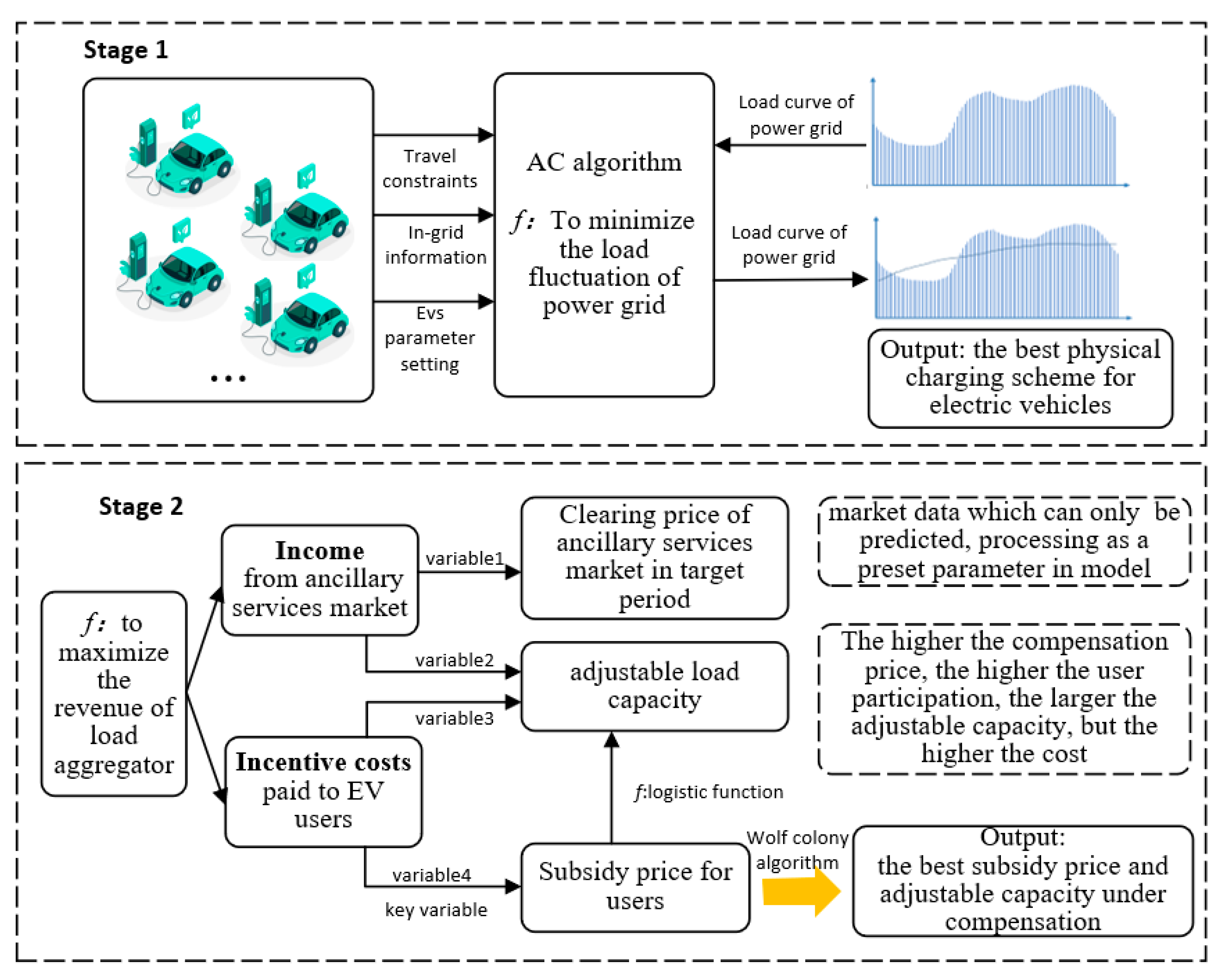
In this paper, an AC network is used to build the charging strategy model of EVs participating in ancillary services.

(1)

Overall structure

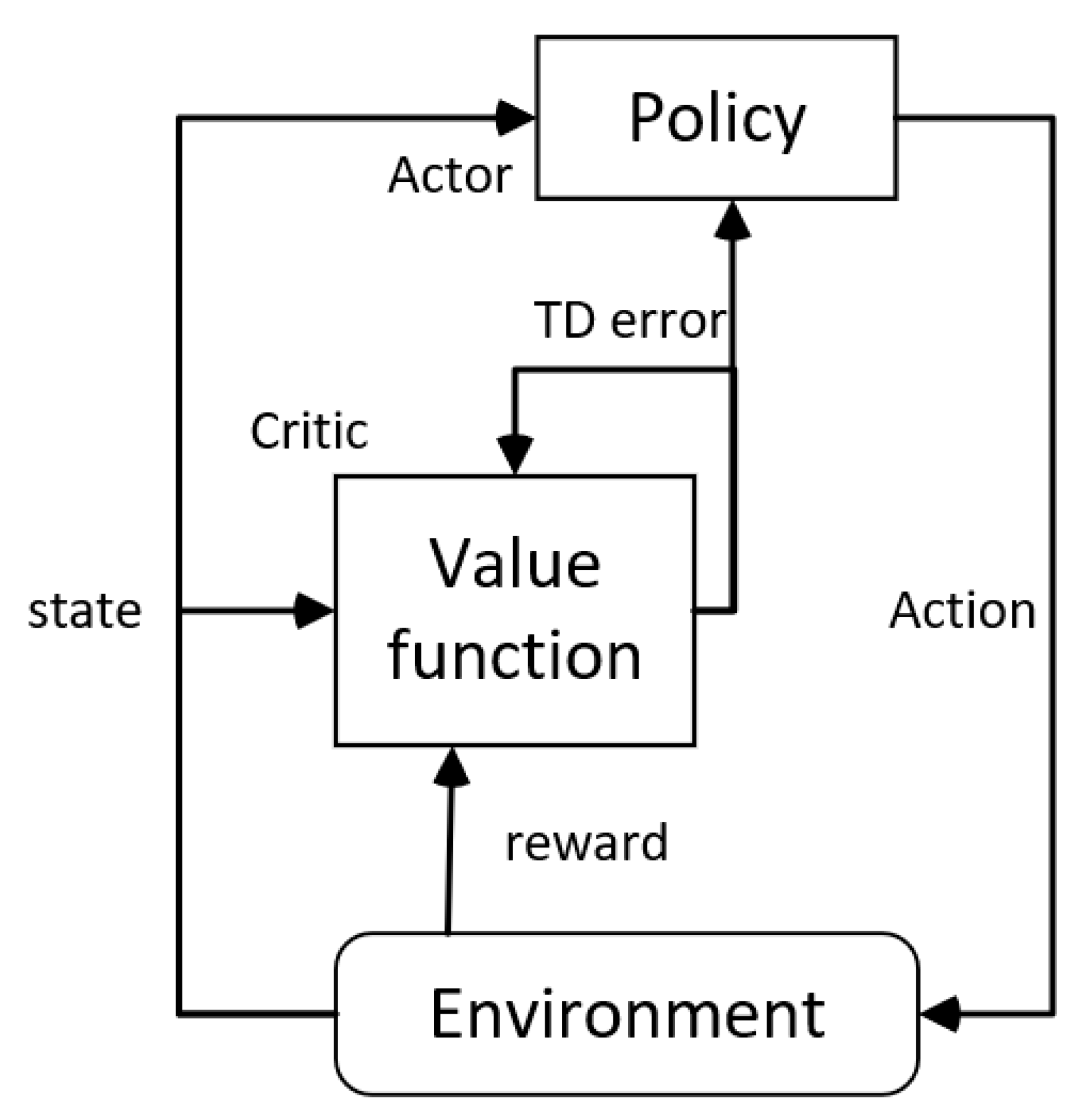
The AC framework is divided into two parts: actor and critic. Both of them are multi-layer BP neural networks. The actor selects behavior based on probability distribution and the critic evaluates score based on behavior generated by actor; the actor modifies probability of selecting behavior according to critic scores. The logic diagram of AC algorithm is shown in Figure 4.

According to the scenario of solving the physical charging scheme of EVs, the AC model environment is built as follows: in the reference state, the EVs start charging after entering the grid or stop charging after reaching the expected SOC. In order to minimize the load fluctuation of EVs after grid connection, it is necessary to optimize the charging power at each time point, so as to obtain the best physical charging scheme. The state characteristics include SOC and charging time. The action distribution is the charging power of EVs at 24 time points, and the reward is the fluctuation of total load variance before and after the EVs enter the grid.

1.

State

$s_t$ is the description of the situation at the current time T. In this paper, a state section t is the state of the t-th EV after accessed to the grid.

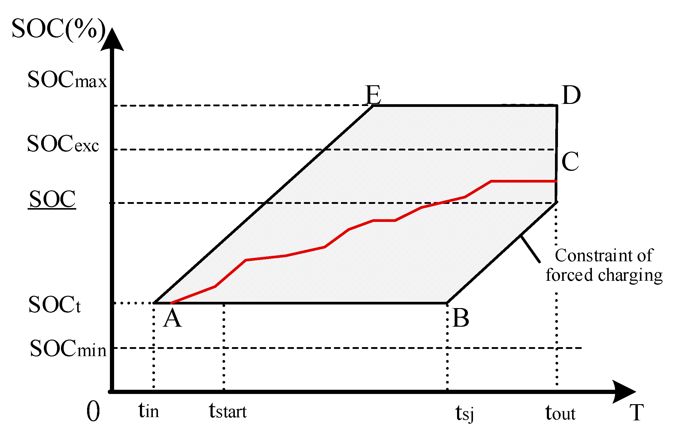
In this paper, for time t, the optimal charging scheme is determined according to its in-grid time t_in, off-grid time t_out, minimum rate of charge threshold SOC_t,min, expected rate of charge SOC_t,exc, off-grid SOC lower bound SOC_t and the latest charging time t_sj. State variables are represented as:

$$s_t=\left[t_{in},t_{out},SO{C}_{t,min},SO{C}_{t,exc},{\underset{\_}{\mathrm{SOC}}}_t,t_{sj}\right]$$

(24)

2.

Action

Action $s_t$ is that at the current time t, the agent observes state $a_t$ from the environment, the response to the environment. The action in this paper shall be the charging power P of EV at all times, expressed as:

$$\begin{array}{c}{a}_t=\left[p_1,p_2,p_3,\dots ,p_{24}\right]\end{array}$$

(25)

3.

Reward

The objective of the agent is to maximize the cumulative reward. According to Formula (4), the optimization objective of the model is to minimize the load fluctuation. Therefore, for a single EV charging scheme, the reward function is set as follows:

$$\begin{array}{c}{R}_t=\frac{1}{24}\left\{{\displaystyle {\displaystyle \sum }_{i=1}^{24}}\left[{\left(Q_{grid,t-1}^i-\overline{Q_{grid,t-1}}\right)}^2\right]-{\displaystyle {\displaystyle \sum }_{i=1}^{24}}\left[{\left(Q_{grid,t}^i-\overline{Q_{grid,t}}\right)}^2\right]\right\}\end{array}$$

(26)

Among them, $Q_{grid,t-1}^i$ and $Q_{grid,t}^i$ is the load at each time point of the power grid in the last observation state and the current observation state; $\overline{Q_{grid,t-1}}$ and $\overline{Q_{grid,t}}$ are the average load of each time point in the last observation state and the current observation state, respectively. In this paper, the load fluctuation caused by the charging scheme under a certain action is taken as a reward, and the variance is used to describe the load fluctuation. The power grid includes the total charging load of EVs and the basic load Q of the power grid $Q_{grid,0}^i$.

(2)

Actor

The Actor is an action output module, whose function is to output the probability of each action by constructing strategy gradient and training, where $v_t$ is the value function generated by the Critic. The loss function of actor network is as follows:

$$\begin{array}{c}\left(\mathsf{\zeta }\right)=lg{\pi }_{\mathsf{\zeta }}\left(S_t,A_t\right)v_t\end{array}$$

(27)

To calculate L (ζ) gradient, which is called the policy gradient of actor network, it can be expressed as:

$$\begin{array}{c}\nabla L\left(\mathsf{\zeta }\right)=\beta {\nabla }_{\mathsf{\zeta }}lg{\pi }_{\mathsf{\zeta }}\left(S_t,A_t\right)v_t\end{array}$$

(28)

where $\nabla$ is the gradient; β represents the learning rate of the strategy gradient, β ∈ (0,1). The gradient descent method is used to train the strategy gradient, and finally the actor network outputs the probability $P\left(A_t\right)$ of different actions.

(3)

Critic

The Critic is a value evaluation module, whose function is to evaluate the value of each action according to the observation value and reward value through time difference algorithm (TD). Its output value is the estimated value of the value function of time difference algorithm, and the value function is transmitted to Actor to provide reference for Actor’s action selection.

The actual value of state action value function of EV cluster at time t is as follows:

$$\begin{array}{c}{Q}_r\left(s_t,a_t\right)=R_{t+1}+\gamma maxQ\left(s_{t+1},a_{t+1}\right)\end{array}$$

(29)

where $Q_r\left(s_t,a_t\right)$ is the actual value of the state action value function; $s_t$ is the state of EV fleet at time t; $a_t$ is the action (charging scheme) selected by the EV group at the time t is the EV individual; $R_{t+1}$ represents the selection of action $a_t$ for the EV fleet in status $s_t$ to state $s_{t+1}$; γ is the discount factor; $maxQ\left(s_{t+1},a_{t+1}\right)$ indicates the maximum value of the state action function of the EV cluster in state $s_{t+1}$.

Discount factor γ indicates the rate at which rewards decay over time steps. That is to say, the further the system state is from the time t, the smaller the interest correlation. When γ = 0, only the current state interests are considered; when γ = 1, the interests of the current state and the future state are equally important.

The method of updating the Q value is as follows:

$$\begin{array}{c}{Q}_k\left(s_t,a_t\right)=Q_{k-1}\left(s_t,a_t\right)+\alpha \left[R_{t+1}+\gamma max{Q}_k\left(s_{t+1},a_{t+1}\right)-Q_{k-1}\left(s_t,a_t\right)\right]\end{array}$$

(30)

where $Q_{k-1}\left(s_t,a_t\right)$ represents the estimated value of the state action value function of the EV at time t in the k-th iteration; α is the learning efficiency, and α < 1.

Let $T{D}_{error}=Q_k\left(s_t,a_t\right)-Q_{k-1}\left(s_t,a_t\right)$ as the loss function of the Critic; the gradient descent method is used to train the Critic.

$${\nabla }_{\theta }J\left(\theta \right)\approx {\nabla }_{\theta }lg{\mathsf{\pi }}_{\theta }\left(a|s\right){\widehat{A}}^{\pi }\left(s,a\right)$$

(31)

$$\theta \leftarrow \theta +\alpha {\nabla }_{\theta }J\left(\theta \right)$$

(32)

At the same time, let $T{D}_{error}$ as the value function $v_t$ in an actor network. The loss function $L\left(\mathrm{Actor}\right)$ of the actor network is:

$$L\left(\mathrm{Actor}\right)=T{D}_{error}·\left[\lg \left(P\left(\delta \right)\right)\right]$$

(33)

The gradient descent method is used to train the loss function of the actor network, and the output is the probability distribution of each action.

To sum up, the logic diagram of the algorithm is given in Algorithm 1:

Algorithm 1: Algorithm flow

Init D  //Initialize policy pool for episode = 1 to $K$ do init Q(S, A)  //Initial action value set $Q_{grid,0}^i$   //Set the basic load of the power grid at all times for $iteration$= 1 to N do   //iteration S = $t_{in},t_{out},SO{C}_{t,min},SO{C}_{t,exc},{\underset{\_}{\mathrm{SOC}}}_t,t_{sj}$   //Collect the information of EVs entering and leaving the grid A = $\left[p_1,p_2,p_3,\dots ,p_{24}\right]$            //Action setting $R=\frac{1}{24}\{{\displaystyle \sum }_{i=1}^{24}\left[{\left(Q_{grid,t-1}^i-\overline{Q_{grid,t-1}}\right)}^2\right]-{\displaystyle \sum }_{i=1}^{24}\left[{\left(Q_{grid,t}^i-\overline{Q_{grid,t}}\right)}^2\right]$  //Reward setting ($S_t,A_t,R_t,S_{t+1})\to D$   //Store data in policy pool mini-batch ($S_t,A_t,R_t,S_{t+1})\leftarrow D$    //Randomly extract data from experience pool for batch gradient descent $Q_{k-1}\left(s_t,a_t\right)\leftarrow Critic-NN$      //The output value of Critic network is the estimated value of action value function $Q_k\left(s_t,a_t\right)=Q_{k-1}\left(s_t,a_t\right)+\alpha \left[R_{t+1}+\gamma max{Q}_k\left(s_{t+1},a_{t+1}\right)-Q_{k-1}\left(s_t,a_t\right)\right]$ //Calculate the target value of action value function $T{D}_{error}=Q_k\left(s_t,a_t\right)-Q_{k-1}\left(s_t,a_t\right)$ //Critic network training error gradient decent$\leftarrow T{D}_{error}{}^2$   //Training critical network with gradient descent method $\lg \left(P\left(\delta \right)\right)\leftarrow Actor-NN$    //The output of actor network is the probability$P\left(A_t\right)$ of different actions_ t) $\mathsf{\zeta }\leftarrow \mathsf{\zeta }|\nabla L\left(\mathsf{\zeta }\right)=\beta {\nabla }_{\mathsf{\zeta }}lg{\pi }_{\mathsf{\zeta }}\left(S_t,A_t\right)v_t$ //To calculate the strategy gradient of actor network gradient decent$\leftarrow {\mathsf{\zeta }}^2$   //To calculate the strategy gradient of actor network end End              //End iteration argmax($P\left(\delta \right)$)$\to record$            //Record the best charging scheme

4.2. Subsidy Price Optimization Algorithm Based on Wolf Colony Algorithm

The wolf colony algorithm is a random probability search algorithm, which can quickly find the optimal solution with a large probability. Moreover, the wolf colony algorithm also has parallelism, which can search from multiple points at the same time, and the points do not affect each other, so as to improve the efficiency of the algorithm [36].

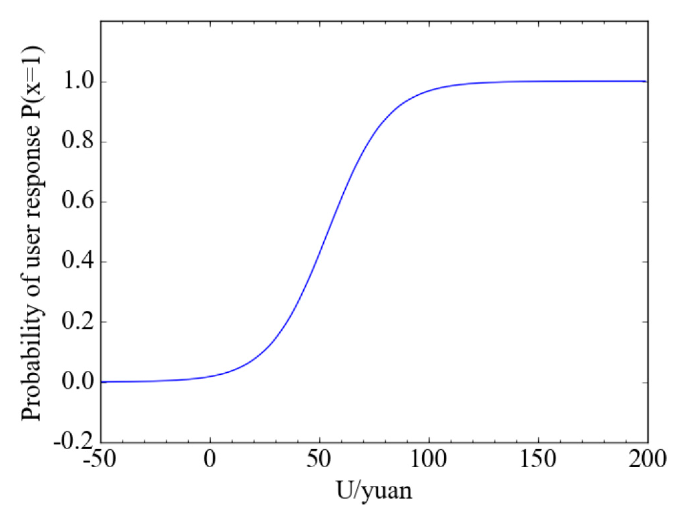
When the charging order has been issued, the EV users will respond according to the subsidy they can get by participating in the response, and choose to accept or not to accept the scheduling. Considering the large number of time-sharing price variables and the number of EVs, and that the price subsidy level at each time point is different, this section uses the optimization ability of the Gray Wolf algorithm to solve the time-sharing subsidy price optimization problem.

(1)

Basic process

Gray Wolf algorithm is an optimization algorithm based on the three links of hunting behavior: tracking, hunting and capturing. According to the fitness value of the whole group, it is divided into leader wolf (head wolf) from top to bottom α, vice chief wolf β, common wolf δ and bottom wolf ω. The leader wolf has the highest fitness value in the group, and plays the role of specifying the moving direction of the wolf group; the ω wolves’ fitness value are low, obeying the law of α, β, δ wolves, and providing stability for the pack. The basic idea of the Gray Wolf algorithm is that α, β, δ wolves locate their prey (optimal solution) and guide ω wolves encircle and hunt.

The process of wolf hunting is as follows:

$$D=\left|C·S_p\left(t\right)-S\left(t\right)\right|$$

(34)

$$S\left(t+1\right)=S_p\left(t\right)-A·D$$

(35)

$$A=2a{r}_1-a$$

(36)

$$C=2r_2$$

(37)

Among them, D is the distance between the individual and the prey, and $X\left(t+1\right)$ is the regeneration position; $S_p\left(t\right)$ represents the position vector of prey (optimal solution), $S\left(t\right)$ represents the individual position vector of gray wolf; C and a are coefficient vectors; $r_1$,$r_2$ is a random number vector with module length between 0 and 1.

The capture activity is mainly realized by the decrement of A. The value of a decreases linearly from 2 to 0 with the number of iterations. In the process of decrement, the corresponding value of A will change between [−a, a]. If $\left|A\right|\le 1$, the next generation of wolves will be closer to their prey; if $1\le \left|A\right|\le 2$, the wolves will disperse away from the prey, resulting in the loss of the optimal solution position and falling into the local optimum. The updating formula of a value is as follows:

𝑎 = 2−2 ∗ 𝑡𝑇

(38)

where t is the current number of iterations and T is the preset maximum number of iterations.

When wolves capture, the location of the wolf $\alpha$, wolf $\beta$, wolf $\delta$ with the highest fitness value is calculated to determine the location of the optimal solution:

$$\{\begin{array}{c}{D}_{\alpha }=\left|C_1·S_{\alpha }\left(t\right)-S\left(t\right)\right|\\ D_{\beta }=\left|C_2·S_{\beta }\left(t\right)-S\left(t\right)\right|\\ D_{\delta }=\left|C_3·S_{\delta }\left(t\right)-S\left(t\right)\right|\end{array}$$

(39)

$$S\{\begin{array}{c}{S}_1=\left|S_{\alpha }\left(t\right)-A_1{D}_{\alpha }\right|\\ S_2=\left|S_{\beta }\left(t\right)-A_2{D}_{\beta }\right|\\ S_3=\left|S_{\delta }\left(t\right)-A_3{D}_{\delta }\right|\end{array}$$

(40)

Finally, the location of the wolves is determined by the wolf $\alpha$, wolf $\beta$, wolf $\delta$:

$$S\left(t+1\right)=\frac{S_1+S_2+S_3}{3}$$

(41)

The fitness function in this paper is the expected profit F of load aggregators participating in the ancillary service market described in Formula (6). The decision variable is the subsidy price at 24 time points, expressed as $s=\left[s_1,s_2,\dots ,s_{24}\right]$, so the position space of the corresponding wolf pack is expressed as an n × 24 matrix.

(2)

Algorithm solving steps

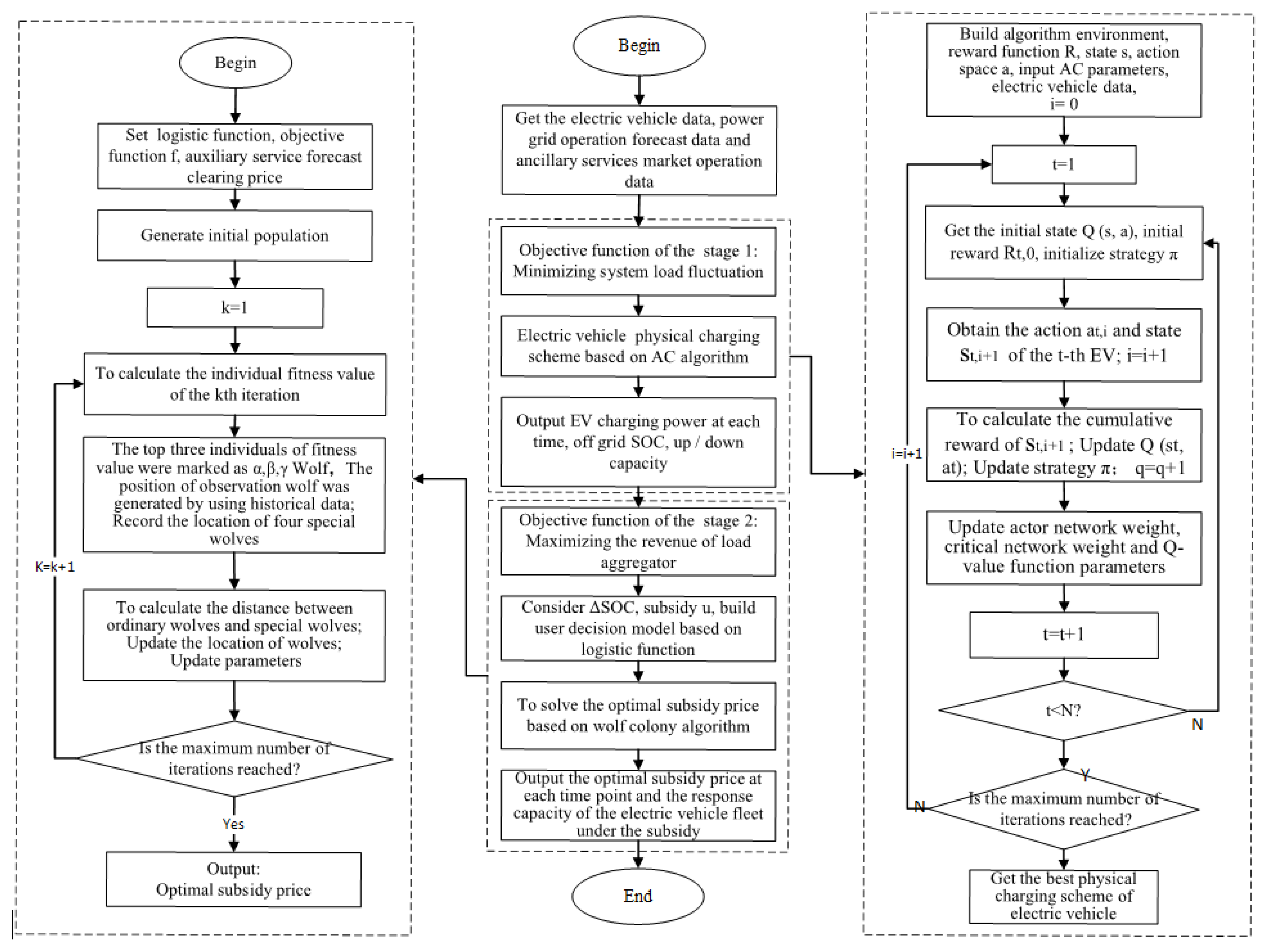
The steps of the Gray Wolf algorithm are as follows:

Step 1: determine the parameters of total overlap algebra K, population size m, etc.;

Step 2: generate the initial candidate price subsidy $S_{m\times 24}$ according to the coding rule of Formula (19);

Step 3: the individual fitness value in the current population is calculated according to the objective function Formula (18) and constraint condition Formula (21); to update the location of wolf $\alpha$, wolf $\beta$, wolf $\delta$, and the position vector of wolf detection is generated according to the historical data;

Step 4: update the position vector of the wolf $\alpha$, wolf $\beta$, wolf $\delta$ and the observation wolf according to Formulas (38)–(39); guide the wolves to update the position according to Equation (40), and update the parameters A and C.

Step 5: if the wolf colony fitness value reaches the maximum number of iterations, the algorithm achieves the expected goal and stops and then goes to step 6; if not, it goes to step 3;

Step 6: the algorithm ends and outputs the individual with the highest fitness value.

In conclusion, the flow chart of two-stage EV physical and economic adjustable capacity evaluation based on AC reinforcement learning and the wolf colony algorithm is shown in Figure 5.

5. Case Study

5.1. Case Design

(1)

Electric vehicle parameters setting

There are 150 private EVs in the set case, and the parameter settings are listed in

Table 1. Characteristic parameters of private EV.

Parameter	Value
Battery capacity/KWH	25
Battery endurance/km	125
Rated power/KW	3.5
Charging efficiency	92%

.

(2)

Description of EV travel characteristics

Based on the literature, the parameters set for the commuting mileage, in-grid and off-grid time of period of ΔT₂ and ΔT₄ are listed in

Table 2. Travel behavior characteristic parameters of private car users.

Parameter	Distribution Characteristics
Commute mileage/km	N (12,1.42)
Time away from home in period ΔT1/h	N (7,1.42)
Off-grid time in period ΔT2/h	N (17,1.22)
Average travel speed in morning peak hours/(km/h)	15.9
Average travel speed in evening peak/(km/h)	15

.

(3)

State of charge of EV

In the ΔT₁ or ΔT₃ period, the EV leaves the grid and enters the discharge state. In the ΔT₂ or ΔT₄ period, EVs are connected to the power grid for charging. The SOC change in EV before and after driving is as follows:

$$SO{C}_{in}=SO{C}_{out}—\frac{dw}{C}$$

(42)

where C is battery capacity, D is commuting distance and W is power consumption per kilometer.

(4)

Parameters of the algorithms

The parameters of AC reinforcement learning and the wolf colony algorithm mentioned in this paper are listed in

Table 3. Algorithm parameters setting.

Algorithm	Parameter	Value
AC algorithm	Iterations	1500
	Data pool capacity	1000
	Number of data randomly extracted	32
	TD learning rate	0.9
	Strategy gradient learning rate	0.1
	Discount factor	1
Wolf colony algorithm	Population number m	20
	Iterations k	200

.

5.2. Case Analysis

(1)

Model solving

The example is set as follows: at the beginning of each travel cycle (at the beginning of ΔT₂), all of them were in full charge state; in the daytime, the SOC_exc required for ΔT₂ is assumed to be 90% when off-grid, while for the ΔT4 at night, it is assumed to be fully charged when off-grid. According to the operation data of the power grid, the power load is divided into three periods: peak period (8:00–11:00, 17:00–23:00), valley period (23:00–5:00 on the next day) and normal period (5:00–8:00, 11:00–17:00), among which peak period opens the peak adjustment auxiliary service market, and valley period opens the valley filling auxiliary service market. The basic load at 96 time points of the power grid is set as

Table A1. Basic load of power grid at 96 time points.

T	Basic Load/kWh	T	Basic Load/kWh	T	Basic Load/kWh	T	Basic Load/kWh
1	15,349.092	25	10,191.08	49	22,852.56	73	24,184.4
2	14,658.904	26	10,350.53	50	22,374.18	74	24,315.79
3	13,977.559	27	10,634.28	51	22,214.69	75	24,446.68
4	13,383.628	28	10,798.42	52	22,021.6	76	24,628.61
5	12,734.614	29	11,343.77	53	21,848.84	77	24,668.85
6	12,335.652	30	12,111.5	54	21,720.22	78	24,897.09
7	12,019.789	31	13,294.8	55	21,525.29	79	25,112.48
8	11,672.977	32	14,378.22	56	21,452.26	80	25,049.7
9	11,339.146	33	15,848.06	57	21,442.45	81	24,862.94
10	11,066.369	34	17,284.01	58	21,371.52	82	24,974.36
11	10,739.833	35	18,628.28	59	21,206.22	83	24,895.81
12	10,619.498	36	19,631.3	60	21,139.79	84	24,550.47
13	10,434.875	37	20,362.84	61	20,996.57	85	24,587.73
14	10,371.812	38	21,208.35	62	21,144.13	86	24,287.23
15	10,156.857	39	21,796.45	63	21,057.62	87	23,855.18
16	10,197.683	40	22,152.55	64	21,323.21	88	23,402.13
17	10,130.988	41	22,461.68	65	21,657.97	89	22,939.91
18	10,030.728	42	22,851.39	66	22,155.76	90	22,272.99
19	10,039.62	43	22,874.18	67	22,582.08	91	21,360.18
20	10,053.83	44	23,176.79	68	22,977.87	92	20,587.81
21	9935.014	45	23,425.78	69	23,189.72	93	19,824.07
22	10,007.253	46	23,431.28	70	23,635.19	94	18,910.71
23	9988.771	47	23,571.22	71	23,765.79	95	18,038.85
24	10,047.398	48	23,154.29	72	23,858.29	96	17,256.7

, Appendix A.

According to the first stage of the model, the reference charging power of EVs fleet and the charging power of EVs fleet in full response are calculated. We can obtain the capacity potential of EVs participating in the regulation according to the instructions. As shown in Figure 6 below, EV charging according to the best charging scheme can effectively pull up the nighttime load trough, reduce the peak charging load and narrow the peak valley difference.

The reward value converges according to Figure 7. The vertical axis represents the cumulative value of the reward.

First, three scenarios are described as follows:

Scene 1: grid reference load without considering EV access;

Scene 2: considering the grid load of EV connected but charging is not regulated;

Scene 3: EVs are charged according to the best physical charging scheme;

According to scene 1, scene 2 and scene 3, peak to valley ratio of daily load in power grid, daily average load, daily load variance of power grid and the load of peak period I (8:00–11:00 in the daytime), peak period II (17:00–23:00 p.m.) and valley period (23:00 p.m.–5:00 p.m.) are calculated and compared for analysis.

It can be seen from the above

Table 4. Comparative analysis of three scenes.

	Peak to Valley Ratio of Daily Load in Power Grid	Daily Average Load of Power Grid/(MWh)	Daily Load Variance of Power Grid	Average Load in Peak Period I/(MWh)	Average Load in Peak Period II/(MWh)	Average Load in Valley Period/(MWh)
Scene 1	0.3956	910.64	71,391.37	846.85	1157.86	621.47
Scene 2	0.3590	1316.06	170,877.9	1313.16	1645.76	863.97
Scene 3	0.4814	1315.36	93,058	1255.34	1575.98	999.02

that the peak to valley ratio of power grid is further reduced from 0.3956 to 0.3550 in the reference state due to the disordered access of EV charging load. Especially, because the charging time of EVs coincides with the peak period of power grid naturally, the load of peak period I and peak period II increases significantly, resulting in “peak on peak”. However, the optimal physical charging scheme can effectively narrow the gap between peak and valley of power grid by regulating EVs and aiming at the minimum fluctuation of power grid. It can be seen from the table that the best charging scheme not only makes up for the increase in peak valley difference caused by disorderly charging of EVs after entering the grid but also effectively reduces the peak load and increases the peak valley load by optimizing the charging time and power of EVs, further reducing the daily peak valley gap and increasing the peak valley ratio to 0.4814.

EV_k, an individual of the EV fleet, is randomly selected for analysis. The information of EV_k is shown in the

Table 5. EV_k process data of ΔT₂ and ΔT₄ after work characteristic parameters of private EV.

Data Name	Value
SOC at in-grid time	0.58
Time when enter gride	10:32
Time when leaves grid	17:12
Commuting distance	23.7 km
Expected SOC when off-grid	0.95
Minimum SOC for the next journey	0.39

below.

From EV_k’s charging data and charging constraints, it can be seen that the SOC of EV is sufficient for the next journey when it enters the grid, and the parking period coincides with the auxiliary service market opening period, so it meets the regulatory conditions. During the period from entering to leaving the grid, the reference charging power and the charging power at each time point under the optimal charging scheme are as Figure 8:

The SOC value of the EV is 0.76 in the evening, which is 0.19 less than the expected SOC. Under the condition that SOC can meet the demand of EVs in the next period of travel, the part of load is transferred to night charging by reducing the charging power in the daytime.

In the second stage, the subsidy is calculated according to the up/down regulated charging power at each time point under the best physical charging scheme of EV, and the subsidy is combined with ΔSOC and substituted into the logistic function to calculate the probability of the user accepting the scheduling scheme. Taking the maximum income of the load aggregator as the objective function, the subsidy price at each time point is determined. Finally, the economic adjustable capacity of EV cluster under the incentive of the subsidy is obtained. Figure 9 shows the best subsidy at each time point.

The ΔSOC and subsidies received by users are substituted into the logistic function to calculate the probability of each user accepting the regulation, and the charging curve of the regulated part is further calculated, shown as Figure 10.

As shown in the figure above, the reason why the economic adjustable capacity is less than the physical adjustable capacity is that the consideration of user decision-making is added. Each EV user makes a decision based on ΔSOC and the subsidy. If the regulation instruction is accepted, the EV will be charged according to the best physical charging scheme, and the rest of the EVs that do not accept the regulation instruction will be charged according to the basic charging curve.

In summary, the regulated EVs are charged according to the issued instructions, and the non-regulated EVs are charged according to the basic charging curve. The total charging curve of the two parts of EVs is the final charging curve of the EV fleet after the economic incentive, as shown in Figure 11.

Because some EVs do not accept the charging scheme, the charging curve under economic incentive is not as good as the best physical charging curve. However, compared with the disorderly charging of EVs, it still effectively increases the load in the valley at night and reduces the load in the noon and evening, which has a significant smoothing effect on the power system operation.

(2)

Sensitivity analysis of logistic function

EV_k travel data and charging data are used to analyze variable parameters β₁, β₂. Sensitivity analysis is carried out to study the influence of variable parameters on the probability P(X = 1) when the subsidy price changes, as shown in the Figure 12 and Figure 13.

(1)

Let coefficient α and β₂ be fixed, as shown in Figure 12: according to Equation (5), β₁ reflects the user’s attention to SOC at the time off-grid. The value of β₁ is larger, indicating that users value SOC more and may have obvious journey anxiety. If the load aggregators want to improve the probability of users’ response of this kind, they can adjust their charging power as far as possible under the condition of meeting their SOC_exc. The change in β₁ does not affect the gradient of the function image P–U, but only makes the image move in the horizontal direction—that is, under the same subsidy price level in a certain range, the smaller the β₁, the higher the probability of users accepting the scheduling.

(2)

Let factor α and β₁ fixed, as shown in Figure 13: coefficient β₂ can affect the skew degree of P–U function image. The larger the value of β₂, the more sensitive the users are to the change in revenue. This type of EV users are usually active in demand-side response; the smaller the β₂ is, the less sensitive the users are to the change in subsidy price, and the load aggregator often needs to pay more cost to motivate such users to participate in the response. Generally, the response of such EVs to economic incentives is lower. In a certain range, under the same level of income, the larger the β₂, the higher the response probability of users.

6. Conclusions

The promotion of EVs is of positive significance to the emission reduction of greenhouse gases and the prevention and control of air pollutants in the transportation industry. However, the growth of power consumption and load brought by the large-scale promotion of EVs in the future will have a profound impact on the generation side, transmission side, distribution side and power supply side. In order to solve this problem, there are some pilot projects in the world that use the flexible adjustable potential of EVs to generate energy exchange with the power grid, and expand the role of EVs from the field of transportation to the two dimensions of transportation energy. The coordinated development of the vehicle grid will not only can provide EVs more friendly access to the grid and reduce obstacles for the rapid development of EVs, but also bring high value to the operation of the power system.

In this paper, we selected private EVs as the research object, and constructed a two-stage physical economic and adjustable capacity evaluation model of EVs for peak load shaving and valley load filling in the ancillary service market. The model is oriented to the scenario of a private EV fleet participating in peak shaving and valley filling of the ancillary service market. In the first stage, the maximum physical adjustable capacity is calculated with the minimum load fluctuation as the goal, and in the second stage, the expected adjustable capacity under subsidy incentive is calculated with the maximum revenue of load aggregators as the goal. Through the model and case analysis, the following conclusions are drawn:

(1)

According to the description of SOC state of EV under the travel characteristics of users, the maximum capacity potential of EVs participating in the ancillary services market is calculated under the condition of meeting the user travel requirements.

(2)

After the EV is connected to the power grid, the user makes a decision whether or not to accept the charging instruction issued by EVA. Considering the user’s decision is directly related to subsidy value and ΔSOC, a user decision model of logistic function is based on these two variables. In the first stage of the adjustable capacity evaluation model, the charging scheme is formulated to minimize the load fluctuation of the power grid and distributed to the EV users. For users, on the one hand, the larger the gap between the participating SOC and the expected SOC, the smaller the user’s desire to participate. On the other hand, the time-sharing subsidy price set by load aggregators directly determines the economic benefits that users can obtain after receiving the adjustment instructions. The higher the subsidy price is, the higher the user participation is.

(3)

The expectation of EV transferable load depends on its maximum capacity potential and user participation. Load aggregators can increase the probability of users participating in ancillary services by increasing the subsidy level, but at the same time, it will increase their own costs. Therefore, the EV load aggregator needs to optimize the time-sharing subsidy price of the EV group under the condition of meeting its own maximum income, so as to maximize the income.

What needs to be supplemented is that although the model can provide reference for the pilot project to a certain extent, it can still be further improved. With the construction of the pilot project, we have more opportunities to obtain the actual operation data, and can use the user’s actual travel data and response data, rather than using statistical data to simulate the actual problems.

References

1. Zechun, H.; Yonghua, S.; Zhiwei, X.; Zhuowei, L.; Kaiqiao, Z.; Long, J. Influence and utilization of electric vehicles connected to power grid. Chin. J. Electr. Eng. 2012, 32, 1–10, 25. [Google Scholar]
2. Haiyang, Y.; Lu, Z.; Yilong, R. Analysis on Influencing Factors of electric vehicle charging behavior based on travel chain. J. Beijing Univ. Aeronaut. Astronaut. 2019, 45, 1732–1740. [Google Scholar]
3. Ciwei, G.; Liang, Z. Overv. of the impact of electric vehicle charging on power grid. Power Grid Technol. 2011, 35, 127–131. [Google Scholar]
4. Pearre, N.S.; Kempton, W.; Guensler, R.L.; Elango, V.V. Electric vehicles: How much range is required for a day’s driving? Transp. Res. Part C Emerg. Technol. 2011, 19, 1171–1184. [Google Scholar] [CrossRef]
5. Andersen, P.B.; Marinelli, M.; Olesen, O.J.; Andersen, C.A.; Poilasne, G.; Christensen, B.; Alm, O. The Nikola project Intelligent electric vehicle integration. In Proceedings of the IEEE PES Innovative Smart Grid Technologies, Istanbul, Turkey, 12–15 October 2014. [Google Scholar]
6. Jochem, P.; Kaschub, T.; Paetz, A.-G.; Fichtner, W. Integrating Electric Vehicles into the German Electricity Grid – an Interdisciplinary Analysis. World Electr. Veh. J. 2012, 5, 763–770. [Google Scholar]
7. Hahn, T.; Schönfelder, M.; Jochem, P.; Heuveline, V.; Fichtner, W. Model-based quantification of load shift potentials and optimized charging of electric vehicles. Smart Grid Renew. Energy 2013, 4, 398–408. [Google Scholar] [CrossRef] [Green Version]
8. Long, J.; Zechun, H.; Yonghua, S.; Huajie, D. Research on joint planning of energy storage and electric vehicle charging station and distribution network. Chin. J. Electr. Eng. 2017, 37, 73–84. [Google Scholar]
9. Hui, H.; Hao, F.; Shu, S.; Zhengtian, L.; Xianbin, K.; Junyang, L. Intelligent charging service strategy for electric vehicles with mutual benefit. Power Syst. Autom. 2017, 41, 66–73. [Google Scholar]
10. Han, S.; Han, S.; Sezaki, K. Development of an optimal vehicle-to-grid aggregator for frequency regulation. IEEE Trans. Smart Grid 2010, 1, 65–72. [Google Scholar]
11. Sortomme, E.; El-Sharkawi, M.A. Optimal charging strategies for unidirectional vehicle-to-grid. IEEE Trans. Smart Grid 2011, 2, 131–138. [Google Scholar] [CrossRef]
12. Pillai, J.R.; Bak-Jensen, B. Integration of vehicle-to-grid in the Western Danish power system. IEEE Trans. Sustain. Energy 2011, 2, 12–19. [Google Scholar] [CrossRef]
13. Tomic, J.; Kempton, W. Using fleets of electric-drive vehicles for grid support. J. Power Sources 2007, 168, 459–468. [Google Scholar] [CrossRef]
14. Li, X.H.; Hong, S.H. User-expected price-based demand response algorithm for a home-to-grid system. Energy 2014, 64, 437–449. [Google Scholar] [CrossRef]
15. Erdinc, O. Economic impacts of small-scale own generating and storage units, and electric vehicles under different demand response strategies for smart households. Appl. Energy 2014, 126, 142–150. [Google Scholar] [CrossRef]
16. Wang, Z.; Wang, S. Grid Power Peak Shaving and Valley Filling Using Vehicle-to-Grid Systems. IEEE Trans. Power Deliv. 2013, 28, 1822–1829. [Google Scholar] [CrossRef]
17. Ge, S.Y.; Liu, J.Y.; Liu, H.; Wang, Y.; Zhao, C. Economic dispatch of energy station with building virtual energy storage in demand response mechanism. Autom. Electr. Power Syst. 2020, 44, 35–43. [Google Scholar]
18. Binbin, Z.; Ying, W.; Xiaomeng, X.; Bin, W.; Wenbo, X.; Zheng, L.; Leijiao, G.E. Load characteristics analysis considering the coordinated dispatching of electric vehicle charging and renewable energy. J. Henan Univ. Technol. 2020, 39, 107–115. [Google Scholar]
19. Lingyun, W.; Xiao, A.; Bo, Y.; Funing, Z. Two level two-stage optimal dispatch of microgrid considering the participation of load aggregators. J. Three Gorges Univ. 2021, 43, 86–92. [Google Scholar]
20. Gang, W.; Weihua, W.; Yan, Z.; Chuanwen, J. Source load interaction bilevel optimization model considering load aggregator participation. Power Grid Technol. 2017, 41, 3956–3963. [Google Scholar]
21. Santos, A.; McGuckin, N.; Nakamoto, H.Y.; Gray, D.; Liss, S. Summary of Travel Trends: 2009 National Household Travel Surve; Federal Highway Administration: Washington, DC, USA, 2011.
22. Hui, W.; Fushuan, W.; Jianbo, X. Analysis of charging and discharging characteristics of electric vehicle and its influence on distribution system. J. N. China Electr. Power Univ. 2011, 38, 17–24. [Google Scholar]
23. Babrowski, O.; Heinrichs, H.; Jochem, P.; Fichtner, W. Load shift potential of electric vehicles in Europe. J. Power Sources 2014, 255, 283–293. [Google Scholar] [CrossRef] [Green Version]
24. Chenghui, T.; Fan, Z.; Ning, Z.; Haoyuan, Q.; Li, M. Day ahead economic dispatch of power system considering randomness and demand response of renewable energy. Power Syst. Autom. 2019, 43, 18–25, 63, 26–28. [Google Scholar]
25. Zhong, C.; Yi, L.; Xuan, C.; Tao, Z.; Qiang, X. Electric vehicle charging and discharging scheduling strategy considering the characteristics of mobile energy storage. Power Syst. Autom. 2020, 44, 77–88. [Google Scholar]
26. Xiaolin, G.; Liang, S.; Ya, L.; Yang, F.; Shu, X. Load forecasting of electric vehicle based on sigmoid cloud model considering demand response uncertainty. Chin. J. Electr. Eng. 2020, 40, 6913–6925. [Google Scholar]
27. Deilami, S.; Masoum, A.S.; Moses, P.S.; Masoum, M.A.S. Real-Time Coordination of Plug-In Electric Vehicle Charging in Smart Grids to Minimize Power Losses and Improve Voltage Profile. IEEE Trans. Smart Grid 2011, 2, 456–467. [Google Scholar] [CrossRef]
28. Haidong, Y.; Yan, Z.; Aiqiang, P. Medium and long term model of electric private car charging load. Power Syst. Autom. 2019, 43, 80–93. [Google Scholar]
29. Jiang, C.; Torquato, R.; Salles, D.; Xu, W. Method to Assess the Power-Quality Impact of Plug-in Electric Vehicles. IEEE Trans. Power Deliv. 2014, 29, 958–965. [Google Scholar] [CrossRef]
30. Azadfar, E.; Sreeram, V.; Harries, D. The investigation of the major factors influencing plug-in electric vehicle driving patterns and charging behavior. Renew. Sustain. Energy Rev. 2015, 42, 1065–1076. [Google Scholar] [CrossRef]
31. Yapeng, Z.; Yunfei, M.; Hongjie, J.; Mingshen, W.; Yu, Z.; Zheng, X. Multi time scale response capability evaluation model of electric vehicle virtual power plant. Power Syst. Autom. 2019, 43, 94–110. [Google Scholar]
32. Delmonte, E.; Kinnear, N.; Jenkins, B.; Skippon, S. What do consumers think of smart charging? Perceptions among actual and potential plug-in electric vehicle adopters in the United Kingdom. Energy Res. Soc. Sci. 2020, 60, 101318. [Google Scholar] [CrossRef]
33. Goebel, C.; Callaway, D.S. Using ICT-controlled plug-in electric vehicles to supply grid regulation in California at different renewable integration levels. IEEE Trans. Smart Grid 2013, 4, 729–740. [Google Scholar] [CrossRef]
34. Jiyun, H.; Jingfei, Y.; Changyi, F. Discharge strategy of electric vehicle charging station based on two-stage optimization model. Smart Power 2021, 49, 83–89. [Google Scholar]
35. Xingyu, Z.; Junjie, H. Deep Reinforcement Learning Optimization Method for Charging Behavior of Cluster Electric Vehicles. Power Grid Technol. 2020, 1–10. Available online: http://kns.cnki.net/kcms/detail/11.2410.TM.20201125.0949.011.html (accessed on 4 May 2021).
36. Husheng, W.; Fengming, Z.; Lushan, W. A new swarm intelligence algorithm wolf swarm algorithm. Syst. Eng. Electron. Technol. 2013, 35, 2430–2438. [Google Scholar]
Figure 1. The logical framework of this paper.
Sustainability 13 08153 g001
Figure 2. Single EV charging load translatable range.
Sustainability 13 08153 g002
Figure 3. The function image of probability P of user accepting scheduling with respect to profit u.
Sustainability 13 08153 g003
Figure 4. AC algorithm model.
Sustainability 13 08153 g004
Figure 5. Flow chart of two-stage EV physical and economic adjustable capacity evaluation based on AC reinforcement learning and wolf colony algorithm.
Sustainability 13 08153 g005
Figure 6. Charging power under reference load and optimal physical charging scheme of power grid.
Sustainability 13 08153 g006
Figure 7. Convergence diagram of AC model algorithm.
Sustainability 13 08153 g007
Figure 8. Reference charging curve and optimal charging scheme curve of t EVk.
Sustainability 13 08153 g008
Figure 9. The best subsidy price in peak and valley period.
Sustainability 13 08153 g009
Figure 10. Physical and economic adjustable capacity of EV.
Sustainability 13 08153 g010
Figure 11. Optimal physical charging curve and final EV fleet charging curve.
Sustainability 13 08153 g011
Figure 12. Sensitivity analysis of parameter β1.
Sustainability 13 08153 g012
Figure 13. Sensitivity analysis of parameter β2.
Sustainability 13 08153 g013