Abstract
Mineral resource estimation involves the determination of the grade and tonnage of a mineral deposit based on its geological characteristics using various estimation methods. Conventional estimation methods, such as geometric and geostatistical techniques, remain the most widely used methods for resource estimation. However, recent advances in computer algorithms have allowed researchers to explore the potential of machine learning techniques in mineral resource estimation. This study presents a comprehensive review of papers that have employed machine learning to estimate mineral resources. The review covers popular machine learning techniques and their implementation and limitations. Papers that performed a comparative analysis of both conventional and machine learning techniques were also considered. The literature shows that the machine learning models can accommodate several geological parameters and effectively approximate complex nonlinear relationships among them, exhibiting superior performance over the conventional techniques.
1. Introduction
Mineral resources are indispensable to the sustenance of modern civilization [1,2]. They play essential roles in socioeconomic development, industrial processes, manufacturing of modern technologies, and construction of modern transportation systems [2,3,4,5]. A mineral resource is commonly defined as “a concentration of naturally occurring material in or on the Earth’s crust in such form and amount that economic extraction of a commodity from the concentration is currently or potentially feasible” [6,7,8]. Evaluation of these resources (mineral resource estimation) is a crucial and challenging task in every mineral exploration and mining project, irrespective of size, commodity, and deposit type [9,10]. Mineral resource estimation is performed to determine the quantity and quality of a mineral deposit and to establish confidence in its geological interpretation, and it requires careful and detailed consideration of high spatial variability and uncertainty associated with geological formations [11]. Therefore, a reliable mineral resource estimate is critical to the success of every mining project.
Mineral resources are subdivided into inferred, indicated, and measured categories based on increasing geological confidence and knowledge, as illustrated in Figure 1 [8]. The estimation of a mineral resource is followed by a mineral reserve estimation, which is carried out to determine the tonnage and average grade of a mineral deposit that is economically and technologically feasible to mine [12]. Mineral resource estimation underlies the generation of mineral reserve estimates. Mineral reserve estimate establishes the mineable portion of a resource and forms the foundation for economic anaslysis of a mineral deposit as well as the future potential of an operating mine. The accuracy of a reserve estimation is essential to the quality of the geological interpretation [13,14]. It is also vital to mine planning and design, including the utility of short-term and long-term mine plans. Moreover, the estimation accuracy is key to mining decisions, such as capital allocation, operating policy, depletion rate, and depreciation charges [13,15,16]. Therefore, an accurate reserve estimation is critical to the feasibility, sustainability, and daily/future operations of a mining project. This phase of the estimation process is also referred to as ore reserve estimation and grade estimation [17]. It should be noted that mineral resource or reserve estimates are not the only factors that determine the extractability of a mineral resource; there are other deciding factors, such as economic, environmental, climatic, and social restrictions [6]. Mineral reserves are classified into probable and proved reserves. Figure 1 shows a general classification of exploration results based on the levels of confidence in geological knowledge and technical and economic considerations about the deposit as established by the Australasian Code for Reporting of Identified Mineral Resources and Ore Reserves (The JORC Code) [17].
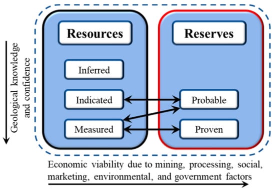
Figure 1.
A general relationship between mineral resources and mineral reserves.
There are two concepts underlying reserve estimation: the concept of extension, where attributes of a sample are extended to blocks to be estimated; and the concept of error estimation, where the validity of an estimation method is assessed based on the error involved [11]. The methods utilized to perform the estimate are important, as they can influence the reliability and accuracy of the estimate. Several estimation methods have been proposed and implemented in the literature. These methods are largely categorized into geometric and geostatistical estimation methods [11,12], and they are termed conventional techniques in this paper. The geometric techniques (e.g., polygonal, triangular, random stratified grids, and cross-sectional methods) are simple and require few input parameters and are often applied at the early stages of a mineral project or to verify the results of the sophisticated estimation methods [11]. However, the geostatistical (e.g., kriging, inverse distance weighting, and conditional simulation) techniques are more sophisticated. The conventional techniques have some inherent limitations. Most notably, they tend to perform poorly with highly heterogeneous datasets, overestimate or underestimate resources, and require significant manual processing [18,19]. Because of these shortfalls, currently, machine learning (ML) methods are being implemented in mineral resource estimation [20,21,22,23,24].
ML techniques are algorithms capable of learning and modeling complex nonlinear patterns in a large dataset [25,26]. Since 1993, many authors have been exploring the potential of ML in resource estimation, resulting in several research publications. Even though the implementation of artificial intelligence and autonomous technologies in the mining industry began decades ago [26,27], it was not until 1993 that ML applications in mineral resource estimation gained enormous research interest. Zhang et al. [28] noted that ML improves resource estimation in the following ways: (i) samples that are rejected in conventional resource estimates because they do not satisfy all quality control requirements can be used provided that the geological descriptions and measurements are reliable; and (ii) resource estimation block models can be constructed using fewer assays and more geology, leading to a reduction in operational costs. Additionally, the ML-based resource estimation approach is significantly cheaper and faster than conventional resource estimation [28]. In addition, ML can modernize hypothesis-testing and geological modeling, contributing to the understanding of various deposit types estimation [28]. Moreover, ML techniques can be employed to address operational challenges and improve safety in different sectors of the mining industry, including mineral prospecting and exploration, mineral evaluation, mine planning, mine scheduling, equipment selection, underground and surface equipment operation, drilling and blasting, mineral processing, and mine reclamation [26,29,30,31].
In addition to assessing the accuracy of different ML and conventional estimation models, these papers examine how various model variables, lithology, and data partition affect model performance. Many of these papers in the literature are spread across various journals and research databases. Therefore, it is imperative these works are consolidated, examined, and compared to form a coherent piece that would inform future research and serve as a reference for interested resource specialists. Our objective is that this paper would provide industry practitioners with an up-to-date knowledge about these emerging techniques and guide them on the choice of the technique applied for different estimation tasks. Additionally, it would also guide researchers to identify new ideas and areas requiring further scientific examination, as the review highlights some limitations and future trends of ML applications in mineral resource estimation.
The remaining part of this paper is divided into five sections. Section 2 outlines the review methodology. Section 3 discusses conventional resource estimation approaches, including geometric and geostatistical methods. Section 4 reviews relevant machine learning techniques that are used for resource estimation. Section 5 presents discussions and highlights key emerging issues that could be the focus of future studies. Section 6 covers concluding remarks.
2. Methodology
2.1. Review Scope
We conducted an extensive literature search to identify relevant peer-reviewed publications indexed in major scientific research databases, such as Web of Science, Google Scholar, Scopus, and ScienceDirect. We used keywords to limit the search scope, including mineral resource estimation, ore grade estimation, reserve estimation, machine learning, soft computing, neural networks, mineral deposit, and support vector machines. Boolean operators (AND, OR, and NOT) and strings (e.g., ‘reserve estimate’) were adopted to improve the search result. Another search strategy employed is snowballing (e.g., forward and backward snowballing), where initial search results lead to the discovery of more papers [32,33].
The search resulted in a plethora of journal, conference, and media publications on mineral resource estimation methods. The result was narrowed solely to peer-reviewed journals, except in a few instances where peer-reviewed conference papers and a Ph.D. dissertation were considered. Only papers published in English have been reviewed, though the search result, especially in Google Scholar, had papers published in other languages. Initial paper selection and review involves content analysis of the title, abstract, and conclusion of a paper to determine if it falls within our review criteria. The review criteria (see Figure 2) are: the paper must be published in a peer-reviewed journal and the content must be related to mineral exploration, especially resource estimation and machine learning. Papers satisfying these criteria were reviewed thoroughly with critical attention to the methods used, algorithm adopted and implementation, findings, conclusion, and recommendation.
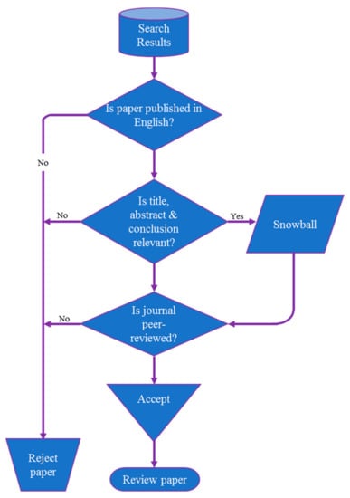
Figure 2.
Review process schematic.
The review covers peer-reviewed publications on machine learning applications in mineral resource, mineral reserve, ore reserve, and grade estimations. For review purposes, we assumed that these different estimation groups deal with the assessment of occurrence, concentration, and tonnage of a mineral in a specific geological location with varying degrees of confidence. These terms are used interchangeably in this article. This general definition affords the flexibility to consider a wide range of relevant publications relating to machine learning and mineral estimation. A conceptual framework of the review process and strategies is illustrated in Figure 2. As indicated in Figure 2, the review process starts with the analysis of search results, which is a collection of papers resulting from a keyword search in various academic databases. Based on the research area/field, the result was streamlined, discarding papers that were not related to the subject matter. Subsequently, the remaining papers were further divided into two main categories: rejected papers and accepted papers. Each paper goes through three consecutive decision questions (language, abstract, and journal type) to determine its category. Papers in the accepted category must pass all the decisions stages; else it is rejected. Snowballing is applied to papers that satisfy the language and abstract stages. Following that, the accepted papers go through a detailed content review.
2.2. Review Summary
The search results included 131 publications. Out of which, 51 were related to machine learning application in mineral resource estimation, while the remaining references cover conventional mineral resource estimation techniques and general knowledge about machine learning. The publication period is limited to 1993–2020; however, a few recent articles published in 2021 were also reviewed. Some of the notable journals where the search results were retrieved include Natural Resources Research, Mathematical Geology, Computers & Geosciences, Computational Geosciences, and Arabian Journal of Geosciences. Figure 3 shows that majority of the ML papers (51 papers) reviewed have been cited multiple times, indicating recognition of these papers by scholars in this field.
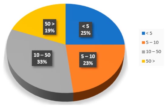
Figure 3.
Citation distribution of ML-based resource estimation papers in this review.
To assess the research trend in this field over the years, the research result (51 papers) was categorized based on the year of publication. Figure 4 shows the distributions of ML-based mineral resource estimation research from 1993 to 2020. It can be observed from Figure 4 that the number of papers per year in the field has experienced two cycles of increase and decrease since 1993, i.e., from 1993 to 2014 and 2015 to 2019. It seems 2020 is the beginning of another surge period, reflecting the increasing research interest in ML techniques in the extractive industry.
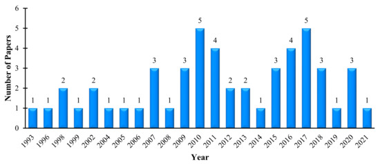
Figure 4.
Trend of publications of machine learning techniques from 1993 to 2020.
Figure 5 presents a summary of the various ML techniques applied in mineral resource estimation. It is interesting to note that artificial neural network (ANN) is the most applied technique, followed by support vector machine (SVM). The remaining techniques are ensemble super learner (Ensemble), inverse distance weighted and artificial neural network (IDW-ANN), genetic algorithms (GA), k-nearest neighbor algorithm (kNN), support vector machines (SVM), support vector regression (SVR), random forest (RF), relevance vector machines (RVM), Gaussian process (GP), and new machine learning-based algorithm (GS-Pred). This is likely due to the strong capabilities of these techniques in pattern recognition and modeling complex systems. These ML techniques allow the modeling of physical features in complex systems without requiring explicit mathematical representations or exhaustive experiments, unlike geostatistical methods. Thus, ML has the potential to provide a more accurate and efficient solution in estimating mineral grades.
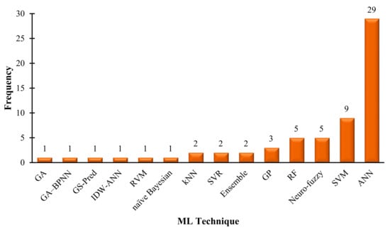
Figure 5.
Distribution of machine learning techniques for mineral resource estimation.
Table 1 details the type of data used for the reviewed ML techniques. The vast majority (more than 80%) were based on field data obtained from exploration drilling (drill cores) or trenching. The significant usage of field data shows the industrial applicability of the proposed ML techniques, suggesting that these techniques can be incorporated in resource estimation tools in the industry. Usage of historical, laboratory, and simulated data account for less than 20% of the implementation. Usually, demonstration using laboratory data involves the acquisition of rock sample images that are subsequently processed with machine vision algorithms. Figure 6 demonstrates the distribution of deposit types analyzed using ML techniques. Interestingly, iron ore and copper deposits are the most evaluated mineral deposits with ML techniques, followed by gold deposits. A summary of the various ML techniques applied to estimate different deposits is presented in Table 2.

Table 1.
Summary of implementation of machine learning techniques.
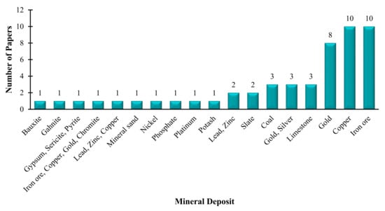
Figure 6.
Distribution of mineral deposits with the machine learning application.
Table 2.
Summary of the various machine learning techniques applied to estimate mineral resources.
3. Conventional Resource Estimation Techniques
In this paper, we referred to conventional resource estimation techniques as geometric and geostatistical methods. These are estimation techniques that are widely applied in mineral deposit evaluation. They have been in use in the mining industry for a long time, and they form the basis of most mineral deposits being exploited today.
The geometric technique includes classical polygon methods, square blocks, rectangular uniform blocks, triangular blocks, and polygonal blocks. These methods, particularly the polygonal approach, have been employed to estimate ore for a wide spectrum of mineral deposits [34,35], and they are most useful at the initial stage of exploration when collated data is relatively small [35]. The basis of this technique is that grades are allocated a definite area of influence generated by constructing the perpendicular bisectors between adjacent samples or intersections to obtain a regional estimate [36,37]. They are conceptually simple, fast, able to decluster irregular data, and adaptable to narrow orebodies, but may not be able to model thick and nontabular orebodies [36].
Geostatistics is a subdivision of statistics concerned with the prediction of random variables associated with spatial and spatiotemporal datasets [38,39]. It has a set of statistical methods that are widely applied in the mining industry, especially for ore grade prediction in mining operations. Other earth science disciplines that apply geostatistics are petroleum, hydrology, and agriculture. Among the various geostatistical techniques, inverse distance weighting (IDW) and kriging are by far the most common method applied in mineral resource estimation [40,41,42].
3.1. Inverse Distance Weighting (IDW)
The IDW methods use the attributes of a known point or sample to interpolate the attributes of an unknown point or block with a weighting factor. According to Chen et al. [43], the assumption is based on the similarity principle that two points maintain similar properties if they are closer to each other. Conversely, if they are farther apart, the weaker the similarities. IDW methods have been successfully implemented to establish ore grades for mineral deposits. Even today, some operating mines use IDW as part of their routine grade control estimation tools due to its low computational cost and easy implementation. Analysis of a survey conducted from 1997 to 1998 indicates that in the Eastern Goldfields of Western Australia, IDW was the most popular grade estimation technique [44]. Dominy and Hunt [44] reported that companies are more likely to employ conventional methods than geostatistical methods in both surface and underground mining operations because some conventional methods have “shown to be historically adequate.” Other reasons for preference of the conventional techniques have to do with company policy or lack of sufficient data to generate a variogram [44].
Yasrebi et al. [45] applied IDW based on combined variograms to generate block models in the Kahang Cu-Mo porphyry deposit in Central Iran. The result from the combined IDW and experimental variogram revealed that the enriched elemental concentrations for Cu and Mo are associated with the central, NE, and NW parts of the area. Shahbeik et al. [40] also employed IDW to establish the ore and waste boundaries for the Dardevey iron ore deposit in Iran. In certain geological settings, IDW is considered an effective alternative to kriging methods. For instance, correlation analysis of IDW and Ordinary Kriging (OK) performed by Al-Hassan and David [46] in evaluating a gold deposit indicates a strong correlation coefficient of 0.93, suggesting that IDW can be used as a good alternative. Again, when compared with OK in limestone deposits [47,48], IDW showed better results, indicating that IDW can be considered a convenient estimation method for limestone deposits.
3.2. Kriging
Kriging has gained enormous recognition in the mining industry and has proven to be a good estimator for mineral resources. Kriging is an estimator designed primarily for local estimation of block grades as a linear combination of available data in or near the block such that the estimate is unbiased with minimal error variance [11,49]. There are many variants of kriging techniques applied in the mining industry, with the most common types being: simple kriging (SK), ordinary kriging (OK), and indicator kriging (IK). Each of the variants differs in underlying assumptions regarding the local or stationary domain mean [11]. Kriging is often associated with the acronym BLUE, meaning the best linear unbiased estimator.
Many scholarly articles have reported kriging, particularly ordinary kriging, as a good estimator for ore reserve estimation [35,49,50,51]. Daya [52] applied ordinary kriging to classify an iron ore deposit. The cross-validation results of his study showed a correlation between estimated and actual data with a correlation coefficient of 0.773. Further, Daya and Bejari [50] compared the performance of two kriging techniques, simple kriging and ordinary kriging, in copper deposits and found that while simple kriging produced a smoother result, the result obtained from ordinary kriging was more accurate. Studies by Hekmatnejad et al. [53] showed that ordinary kriging also compares well with non-linear kriging techniques (e.g., disjunctive kriging). However, in some instances, disjunctive kriging may outperform ordinary kriging [53]. Other advanced kriging techniques, such as fuzzy kriging and compositional kriging, have also shown reliable results. For example, Taboada et al. [54] modeled and zoned a quartz deposit in Sierra del Pico Sacro, Spain, into four different quality grades (silicon metal, ferrosilicon, aggregate, and kaolin) using compositional kriging. The result was considered satisfactory as it matched the geological reality of the deposit.
4. Machine Learning Techniques
The increased interest in machine learning (ML) in recent years is reflected in the growing numbers of scholarly publications about its application in geoscience. ML techniques cover a broad spectrum of geoscience applications, ranging from identifying geochemical anomalies to evaluating mineral resources. ML techniques are not new in the extractive industry; however, their application has surged during the last decade due to promising results to complex problems in the industry. ML is the study and application of computer algorithms to make intelligent systems that improve automatically through the experience without being explicitly programmed [25]. It is classified as a subfield of artificial intelligence (AI), which is the science and engineering of making intelligent machines. ML applies computer algorithms to analyze and learn from data, to decide or predict outcomes in various fields depending on the structure of available data being analyzed. ML models are categorized as supervised learning, unsupervised learning, and reinforcement learning [55]. Each of these classes is further categorized, based on the nature of the problem being solved, using various corresponding learning algorithms or applications to handle such problems. In practice, there are many ML algorithms applied in engineering fields; however, only those commonly applied to mineral resources estimation problems are considered in this paper.
A generalized ML implementation process is presented in Figure 7. The first step in the ML model development cycle (problem definition) deals with understanding the problem, characterizing it, and eliciting required knowledge in acquiring the relevant data. The second step (data collection) involves the collection of all relevant data based on the features prescribed in the first step, followed by data preparation, pre-processing, and transformation. Feature selection deals with automatic or manual selection parameters or variables that contribute most to the prediction variable or output of interest. Next, the data is divided into training, validation, and testing sets based on a predefined ratio (data partition). Typically, 60% of the data is used for training, 20% for validation, and 20% for testing. Following that, an ML model is trained, validated, and tested using the partitioned datasets (train model). Model evaluation involves the usage of new sample data to re-verify the model performance. The model parameters (e.g., number of training steps, learning rate, initialization values) can be revised until a satisfactory performance is achieved, and then the model can be deployed for prediction.
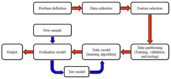
Figure 7.
Machine learning implementation stages.
Prominent among ML methods (see Figure 8) that have been employed to estimate mineral resources are artificial neural network (ANN), support vector machine (SVM), random forest (RF), gaussian processes (GP), and fuzzy theory sets. These models have been successfully applied in evaluating different mineral deposits, including limestone, gold, and copper. The proceeding subsections review application of these algorithms to mineral resource estimation problems. There is extensive documentation in the literature regarding assumptions, mathematical computation, and architecture of these techniques; thus, this paper focuses largely on their application.
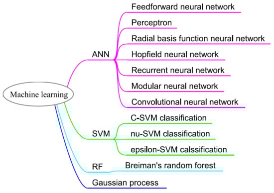
Figure 8.
Machine learning techniques and their corresponding algorithms.
4.1. Artificial Neural Network (ANN)
ANN is a computational network presenting a simplified abstraction of the human brain. Conceptually, this computational network mimics the operations of biological neural networks to recognize existing relationships in a set of data and predict output values for given input values. It consists of layers of interconnected nodes, which represent artificial neurons [56]. The layers are categorized into three divisions; input layer (receives the raw data), hidden layer (process the raw data), and output layer (processed data). The number of layers and neurons (topology) in a network determines the structure of a neural network or network architecture. Figure 9 illustrates a basic ANN architecture comprising an input layer with three variables, a hidden layer with two neurons, and an output layer with one variable. Further, the neural network layers are transformed into a computational network made up of weight, bias or offset, and transfer or activation function that are responsible for data processing.
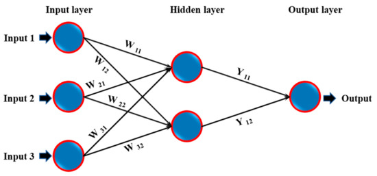
Figure 9.
Simplified ANN architecture with a single hidden layer.
Increasingly, ANN has infiltrated many engineering and statistical applications involving clustering, regression, forecasting, signal processing, and modeling problems. The wide recognition for ANNs could be attributed to their ability to learn and model complex non-linear relationships and make generalizations after learning from previous data [57]. There are several types and modifications of ANNs in practice today for different problems in geoscience, including multilayer perceptron (MLP), radial basis function (RBF) networks, general regression neural networks (GRNN), probabilistic neural networks (PNN), self-organizing Kohonen maps (SOM), Gaussian mixture models (GMM), and mixture density networks (MDN). In mineral exploration, ANNs have been widely applied for solving complex geospatial problems, such as prospectivity of mineral resources [58,59], mapping of mineral resource distribution [60,61,62], classification of mineral deposit [63,64], and mineral recovery [65]. Given their strong ability to manipulate large and complex data structure, reason over imprecise and fuzzy data, and to provide adequate and quick responses to new information [66], ANN is considered to be a robust alternative to geostatistical methods for evaluating mineral resources and reserves [67,68,69].
Generally, geological information, such as spatial location and assay results obtained from exploration programs, forms the basis of ANN models in resource estimation. The spatial location of the borehole usually presents the input layer, while the output layer accounts for the ore grade. Wu and Zhou [37] implemented a multilayer feed-forward neural network with a sigmoid activation function to capture spatial distributions of grade based on field assay of borehole locations in a copper deposit. The network architecture comprises an input layer with two variables (borehole coordinates), two hidden layers with 28 neurons each, and an out layer with one variable (ore grade). Al-Alawi and Tawo [66] demonstrated the potential of ANN to determine suitable drilling patterns and eventual reduction in exploration cost. They developed a multilayer feed-forward ANN-based model with a back-propagation algorithm to estimate point grades for a bauxite deposit. The model, which showed reasonable agreement with kriging, was applied to unsampled points to determine feasible areas for infill drilling. Further, Tahmasebi and Hezarkhani [70] employed a modular feed-forward neural network to estimate the grade of an iron ore deposit with improved performance compared to ordinary kriging and conventional multilayer perceptron neural networks. In a slate deposit, Matías et al. [71] determined the quality of slate mine using regularization networks (RN), multilayer perceptron (MLP), and radial basis function (RBF) network and compared the accuracy of the models with kriging.
Studies have also gone beyond the usage of borehole locations as input variables to incorporate other relevant geological attributes such as lithology and alteration obtained during exploration. Ore deposits with varied grade attributes (i.e., output layer with multiple nodes) are possible to model with ANN. For instance, Chatterjee et al. [72] modeled a limestone deposit using a feed-forward neural network where the input layer consists of spatial location (X, Y, and Z coordinates) and lithological information, and the output layer of four grade types (silica (SiO2), alumina (Al2O3), calcium oxide (CaO), and ferrous oxide (Fe2O3)). The ANN model showed superior performance when compared with ordinary kriging. Kaplan and Topal [73] proposed a grade estimation technique that combines multilayer feed-forward neural network (NN) and k-nearest neighbor (kNN) models to estimate the grade distribution within a mineral deposit (see Figure 10). The models were created using lithology, alteration, and sample locations (easting, northing, and elevation) obtained from the drill hole data. The proposed approach explicitly maintains pattern recognition over the geological features and the chemical composition (mineral grade) of the data. Before the estimation of grades, rock types and alterations were predicted at unsampled locations using the kNN algorithm. The result showed that inclusion of the geological information (lithology and alteration) as input parameters improved the model, which had a mean absolute error (MAE) of 0.507 and coefficient of determination (R2) is 0.528, whereas the ANN model that only uses the coordinates of sample points as an input yielded an MAE value of 0.862 and R2 = 0.112.
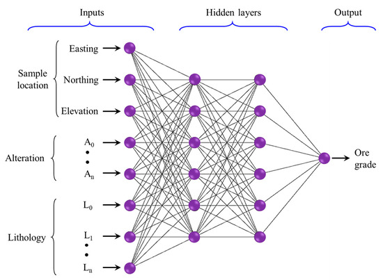
Figure 10.
Proposed NN model architecture, adapted from [73].
More recently, fuzzy uncertainties associated with geological data are being modeled with hybrid neural-fuzzy algorithms [74,75,76,77,78] to quantify uncertainties in evaluating mineral inventory parameters. Similar ANN-based mineral estimation models include Wavelet neural network (WNN) for copper deposit [79], recurrent neural network (RNN) for iron ore deposit [80], Kalman learning algorithm (modified back-propagation neural network) for lead (Pb), and zinc (Zn) deposit [81], local linear radial basis function (LLRBF) neural network for phosphate deposit [82], and radial basis function (RBF) network for offshore placer gold deposit [83,84]. Table 3 shows a summary of some ANN-based resource estimation models.
Table 3.
Sample case studies of ANN-based mineral resource estimation.
4.2. Support Vector Machines (SVM)
Another machine learning technique gaining significant attention in resource estimation is support vector machines. SVMs are supervised learning models that construct a hyperplane in high dimensional feature space to separate different classes through non-linear mapping [85]. Given a set of training examples, which belong to different categories, an SVM model constructs a separating line with a gap between the data categories. The model then maps new examples into the same space and predicts the respective side of the separating line or category. SVMs are becoming popular for solving classification, regression, and outlier detection problems. According to Chatterjee and Bandopadhyay [86] and Xiao-li et al. [87], SVMs function just like ANN, but with the added advantages of achieving global minimum and efficient handling of over-fitting problems; hence their growing prominence in mineral exploration applications is evident. Examples of SVM application in mineral exploration include: mineral prospectivity [88,89], potential mineralized zones mapping [90,91,92], fluid inclusion modeling [93], exploration drill holes location identification [94], alteration zone separation [95], and slate deposit characterization [96].
Further application of SVM in mineral exploration has to do with resource estimation. Das Goswami et al. [97] employed support vector regression (SVR) to model an iron ore deposit. They assessed the grade of the deposit and compared the model with gaussian process regression and ordinary kriging. The model output (Fe grade) was determined using spatial coordinates (X, Y, and Z) and ten lithological features as input. As demonstrated by Chatterjee and Bandopadhyay [86], SVM has also proven to be sufficient for evaluating placer deposits, which are often sparsely sampled, increasing the complexity of the estimation process. Using exploration data from a platinum deposit, the authors adopted least square support vector regression (LS-SVR) and combined neighboring borehole samples as the model input instead of the conventional spatial coordinates to estimate the ore grade. The improved estimate result of the model compared with conventional SVM and ordinary kriging was attributed to the composting of neighboring samples. Further improvement was expected with an increase in neighbor samples. Similarly, Zhang et al. [98] applied least square support vector regression to the model to estimate the ore grade of a seafloor hydrothermal sulfide deposit. The model demonstrated superior results in comparison to inverse distance weight (IDW), ordinary kriging (OK), and back-propagation (BP) neural network, and showed robust predictive and generalization ability.
During exploration drilling, there are instances where drill cores cannot be recovered, resulting in missing data and incomplete core samples. This situation complicates the estimation process and may eventually render the result inaccurate. To solve this estimation problem, Zhang et al. [99] incorporated a relevance vector machine (RVM)–a modified version of SVM based on Bayesian treatment [100]–and expected squared distance (ESD) algorithms to determine the missing values and estimate the ore grade. Li et al. [87] also proposed an integrated model of self-adaptive learning-based particle swarm optimization (SLPSO) and support vector regression (SVR) for porphyry copper ore grade estimation. Table 4 presents a summary of SVM-based resource estimation models.
Table 4.
Sample case studies of SVM-based mineral resource estimation.
4.3. Random Forest (RF)
Random forest is an ensemble learning technique consisting of collection decision trees that are trained using random training subset to output mode class in classification and mean prediction in regression problems [101,102]. Each decision tree outputs a class, and the class with the most votes is the model’s prediction. Since the final output is a combined decision, it most likely outperforms the prediction of an individual tree. The decision trees are constructed by bagging or bootstrap aggregation, meaning the samples are drawn from a subset of training data with replacement. Figure 11 illustrates a schematic framework of RF with five samples and three variables. In Figure 11, the trees are created in an ensemble by drawing a subset of training samples through replacement, meaning that the same sample can be selected several times, while others may not be selected at all (i.e., training phase). Then, each tree votes for a class membership, and the membership class with the maximum votes will be the one that is finally selected (i.e., classification phase). Studies have shown that RF has several desirable qualities, including handling large data sets efficiently; ability to detect outliers and noise; capacity to produce suitable internal estimates of generalization error; and computationally cheaper than bagging or boosting [101,103,104,105].
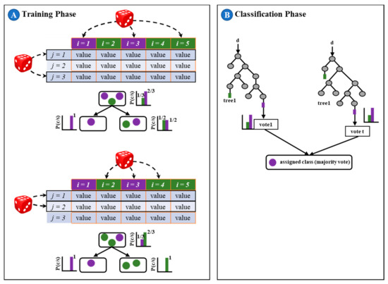
Figure 11.
Random forest classifier schematic: i = samples, j = variables, p = probability, c = class, s = data, t = number of trees, d = new data to be classified, and value = the different values that the variable j can have, adapted from [106].
In addition to its enormous application in areas, such as land cover classification [104], groundwater modeling [107,108], and mineral prospectivity [89,109], RF is gaining popularity in predicting the ore grade of mineral deposits. For example, Jafrasteh et al. [110] investigated the potential of an RF-based model for evaluating grades of porphyry copper deposit and the model’s performance with other machine learning algorithms (e.g., multilayer perceptron neural network) and geostatistical techniques (e.g., indicator kriging, and ordinary kriging). The RF-based model was made up of hyper-parameters that were adjusted by 500 decision trees sufficient to ensure convergence of the model. Sheng et al. [111] combined laser-induced breakdown spectroscopy (LIBS) and random forest (RF) to classify iron ore samples with 100% prediction accuracy. In another study, O’Brien et al. [112] classified gahnite compositions of the Broken Hill deposit to determine most prospective Pb-Zn-Ag mineralization in the Broken Hill domain, Australia. The results show that RF is a better technique for compositional discrimination in the Broken Hill domain compared with linear discriminant analysis. In an exploration study, Schnitzler et al. [113] used RF to assess sodium (Na) concentration in the Matagami mining district of Québec, Canada and illustrated that RF could be an efficient tool for estimating missing or unmeasured geochemical elements in an exploration database. Matin and Chelgan [114] also alluded to the potential of RF to model complex relationships in their study to investigate gross calorific value of coal samples from 26 US states, where it was applied with satisfactory results. Table 5 summaries RF-based resource estimation models.
Table 5.
Sample case studies of RF-based mineral resource estimation.
4.4. Emerging and Hybrid Algorithms
There are other machine learning techniques being applied to mineral resource estimation problems, though they are not widely used compared to the above-mentioned machine learning models. Gaussian processes [115,116], for instance, is popular in geoscience, especially for geochemical anomaly detection [117,118] and mineral prospectivity studies [119,120], but we observed in the literature that it had been applied once to estimate ore grade of a deposit [110]. Jafrasteh et al. [110] suggested that GP models gave the best results when spatial input and covariance functions were processed using symmetric standardization (SS) and anisotropic exponential kernel (AK), respectively. Thus, in their experimental study, they applied GP with symmetric standardization and an anisotropic exponential kernel GP to evaluate the grade of a copper deposit. And as expected, the GP-SS-AK algorithm performed well among other GP algorithms, including the exponential kernel, isotropic exponential kernel, symmetric standardization, and anisotropic exponential kernel.
Recently, researchers have been exploring the potential of incorporating machine learning techniques with other sophisticated soft computing methods (e.g., genetic algorithm, ant colony, fuzzy set theory, etc.). The aim is to synthesize the advantages of these algorithms to build a single algorithm with improved accuracy for resource estimation. Examples of these models include grade estimation of copper deposit using self-adaptive learning-based particle swarm optimization and support vector regression (SLPSO–SVR) [87]; multilayer perceptron neural network optimized by invasive weed optimization algorithm to predict grades of gold and silver in gold deposit [121]; local linear radial basis function neural network trained with a combination of simultaneous perturbation artificial bee colony algorithm and back-propagation method to estimate phosphate deposit [82]; combination of multilayer perceptron neural network and genetic algorithm for an iron deposit [122]; and extreme learning machine (ELM) variants based on hard limit, sigmoid, triangular basis, sine and radial basis activation functions to gold deposit [19]. Yu et al. [123] optimized iron ore grades using a combination of stochastic simulation, artificial neural network, and genetic algorithm. Further, given the potential of computer vision methods, studies, such as Chatterjee and Bhattacherjee [124], Patel et al. [125], Patel and Chatterjee [126], Perez et al. [127], and Zhang et al. [128] also integrated image recognition algorithms with other machine learning methods to classify and predict ore grade. Table 6 presents a summary of some of the emerging ML techniques applied in estimating mineral resources.
Table 6.
Sample case studies of emerging machine learning techniques for mineral resource estimation.
5. Discussion and Future Directions
The continued advancement in computer power has unraveled novel and sophisticated soft computing techniques capable of handling large and complex dimensional data structures that were not possible in the past. These soft computing techniques include machine learning coupled with big data technologies to create a new paradigm of powerful resource estimation models. Machine learning applications have infiltrated all fields and industries, from engineering to sociology, agriculture to astronomy. Some scholars even refer to it as the new electricity driven by data. Geoscience has also witnessed tremendous advances with the onset of ML. There is a consensus among geoscientists that ML algorithms are suitable for geospatial data that often exhibit complex and high spatial variations [129,130,131], and the algorithms can produce superior results for classification and regression problems than geostatistical techniques, especially when the relationship is non-linear [132,133,134,135,136,137]. Some of the ML algorithms are universal, adaptive, non-linear, robust, and efficient [129]. Another favorable characteristic of ML is that it allows the discovery of new information or a deeper understanding of existing geospatial data. This is evident in the assertion by Nwaila et al. [138] that the advent of ML made sedimentological data, which were initially collected for qualitative assessment of gold mineralization, more meaningful and contextually relevant. ML-based estimation algorithms can accommodate a combination of several geospatial parameters for grade prediction and ore classification. In addition to the spatial location of drill holes and composite grade, lithological, geochemical, and rock imagery features, which are often overlooked or not accommodated in geostatistical techniques, can be included in the dependent variables of the model [139], resulting in a more improved estimation model. The main appealing features of ML for resource estimation, in contrast to conventional estimation techniques, are that it (i) requires fewer data pre-processing, (ii) handles complex non-linear relationships, (iii) relatively cheaper and faster, and (iv) does not assume underlying spatial distribution and handles incomplete data.
Despite the strong potential of ML and its recent increasing application in the evaluation of mineral resources, geostatistical methods remain the benchmark estimation technique in the mining industry. ML techniques are considered more of a complementary tool for validating results obtained from geostatistical methods than sole estimation techniques for mineral projects. Glacken & Snowden [36] noted that many estimation tasks are still conducted using polygonal techniques regardless of the availability of sophisticated estimation methods. The high preference for geostatistical techniques may be because they have been applied in the industry for a long period, forming the basis for many mine designs in operation today. In addition, their underlying framework of linear correlation of samples and stationarity [97,133,140] makes them less computationally expensive compared to ML techniques. Furthermore, they can be integrated with other statistical concepts, for example, conditional simulation, which is a combination of kriging and the Monte Carlo sampling method [36]. Moreover, many resource engineers have gained comprehensive experience over the years in applications of these methods with reliable results. Thus, they would be more comfortable working with techniques that are widely accepted in the industry. Stakeholders also have confidence in these techniques.
Additionally, most geostatistical algorithms have been automated in modern mineral resource software packages (e.g., Datamine, GEMS, Leapfrog, Micromine, Surpac, Vulcan, etc.) for easy data manipulation and estimation. This allows the estimators to focus more on the data preparation and result interpretation. Another reason could be that geostatistical techniques are widely recognized by the Committee for Mineral Reserves International Reporting Standards (CRIRSCO) members and their respective mineral resources and ore reserve estimation reporting schemes, such as National Instrument 43–101 in Canada, Joint Ore Reserves Committee Code (JORC Code) in Australia, South African Code for the Reporting of Mineral Resources and Mineral Reserves (SAMREC) in South Africa, SME Guide in the USA, NAEN Code in Russia, and Pan-European Reserves and Resources Reporting Committee (PERC) in Europe and the United Kingdom.
Although geostatistical techniques are the industry’s estimation standard, they possess certain inherent limitations. As mentioned earlier, these methods are generally linear estimators; thus, grades of unknown samples are determined based on second-order statistics and the use of linear correlation or variogram, which describes mineralization of a deposit [97]. According to Das Goswami et al. [134], second-order statistics work reasonably well with statistical processes following the Gaussian process. Nonetheless, it is difficult to model complex geological structures with high variability that do not follow the Gaussian process. Tutmez [76] also pointed out that geostatistical methods perform poorly on small data sets (i.e., not enough data to achieve acceptable variogram calculation). Therefore, they are not suitable for small deposits or during the initial exploration stage, where data is limited. They also require significant data-processing [137]. In such situations, ML techniques can be adopted.
ML techniques are known to sufficiently handle spatial uncertainty associated with geological data [89,97,133,141] sbecause of their ability to determine the relationship between complex and non-linear input and output variables [97]. ML techniques can learn and map inherent relationships among the data variables. Given enough geological data (such as drill hole coordinates and assay results), ML techniques can learn the relationship between input parameters (coordinates of drilled holes) and output parameters (ore grades). The trained model can then be used to estimate grades for unknown points within the same geological area. In effect, no assumption is made about factors or relationships of ore grade spatial variations, such as linearity between drilled holes [133] as in the case of geostatistical techniques. Several case studies (see Table 3, Table 4, Table 5 and Table 6) have illustrated the potential of ML techniques as a good estimator of ore grade for different mineral deposits; some studies have done so by comparing its performance with geostatistical techniques.
Results from studies comparing the performance of both models are mixed. In some cases, geostatistical techniques showed better output and vice versa. In other words, there is no outright best method between the two, and they seem to complement each other. Generally, the ML techniques seem to have higher accuracy than the geostatistical methods. When Das Goswami et al. [97] compared two ML techniques (general regression neural network (GRNN) and multilayer perceptron neural network (MLPNN)) and one geostatistical technique (ordinary kriging (OK)) in an iron deposit, they found that GRNN exhibits better generalization potentials and also provides higher accurate prediction than MLPNN or OK models. MLPNN and OK were also observed to overestimate lower grades and underestimate the higher grades, while GRNN showed minor variation between the predicted and actual iron grade. In the Nome gold ore reserve estimation, Dutta et al. [102] demonstrated that SVM produced better estimates compared to ANN and OK. Afeni et al. [142] re-examined grade estimates for an iron ore deposit using MLPNN and OK and observed that the OK model showed superior performance than the MLPNN model. The total resource definition by OK was about 12% lower than that of the conventional method currently used in the mine. Karami and Afzal [101] also evaluated the performance of ANN and IDW on a copper deposit and reported that the IDW method showed less variance, while ANN demonstrated high overestimation and underestimation. Thus, in this instance, IDW is a better estimator than ANN. In Kaplan and Topal’s [73] study, the NN and kNN model underestimated any grades between the 15 ppm and 20 ppm range. Upon close examination of sample points, they observed that the network could not ignore the effect of discontinuity of lithology in areas where mineralization is structurally controlled and a test point located near a fault; thus, the model is more suitable for mineralization controlled by lithology than structure.
It is worth mentioning that ML techniques are not a panacea to all resource estimation problems, as they also have limitations. Jafrasteh et al. [115] indicated that ML techniques are effective only if the training and test datasets have similar distributions. The models tend to perform poorly when the samples are far apart with increasing spatial variation. Thus, the training data and test dataset must be carefully partitioned to ensure that they have the same or similar geological characteristics. This problem can be resolved by assigning a higher weight to training samples closer to the test samples [141]. Kapageridis [143] observed that the dimension of input data influenced the performance of ML techniques, particularly ANN applied to ore grade estimation. After examining 2D and 3D spaces with varying input configurations, ranging from two to sixteen input dimensions on different deposit types (potash, marl, phosphate, and copper), the author concluded that for ANN, “there is no globally applicable configuration for all deposit and sampling scheme types, and each deposit and sampling scheme must be considered separately to find the best configuration applicable.” The adopted input dimension can either hurt performance when available data is small or improve when available data is large enough. Thus, it can be inferred that there is no one-fit-all ML technique for all resource estimation problems, but the choice of technique is contingent on available data and deposit characteristics. Further, we observed that many ML-based grade estimation models are limited only to geological parameters (e.g., using only spatial coordinates). Erdogan Erten et al. [144] corroborate this observation, stating that “ML models provide useful tools to generate spatial estimations of geological features, but they do not consider the spatial dependence among the observations and they primarily use coordinates as predictors. Thus, many ML models produce visible artifacts in the resulting estimates along the coordinate directions.” The authors proposed using ensemble super learner (ESL) to address this weakness.
Again, ML algorithms that focus on finding the best solution for a model tend to overfit or underfit because the optimum model for training and testing the dataset may not necessarily have the best generalization ability [145]. This problem can be addressed using ensemble methods, where multiple learning algorithms are applied with different parameters, and the resulting solutions are averaged to obtain better performance than any of the constituent learning algorithms [146,147,148]. Examples of this learning method are Bayes optimal classifier, bootstrap aggregating (bagging), boosting, Bayesian model averaging, bucket of models, and stacking. Chatterjee et al. [148] investigated the performance of genetic algorithms and k-means clustering based on an ensemble neural network for a lead-zinc deposit. The result showed no significant difference in the model performance. They attributed the marginal performance to the high coefficient of variations and skewness of the data sample. But Tahmasebi et al. [78] pointed out that, perhaps, optimizing ANN’s parameters and topology could have improved the result. An earlier study conducted by Tahmasebi and Hezarkhani [149] showed better results when the ANN’s parameters and topology were optimized with genetic algorithms.
Another critical factor observed to influence the accuracy of ML-based estimation models is data partitioning [110,150]. Most studies assume random partitioning to divide the sample data into training (e.g., 60%), validation (e.g., 20%), and testing (e.g., 20%). However, due to variation in drillhole samples (in both 2D and 3D) and erratic distribution of geochemical anomalies, such an approach may bias model performance as closer holes tend to exhibit similar features than farther holes. Thus, it is important to consider lithological features and other inherent characteristics particular to the formation when deciding which data partition regime to adopt. Additionally, instead of using composite values, individual drillholes can be modeled along the z-axis based on core sample intervals. The result obtained from each local drillhole model can be synthesized as input-output parameters for the global model. This would mimic spatial distribution along the drillholes, allow the inclusion of more features, produce more realistic models, and improve performance and accuracy.
ML is data-driven, requiring a large dataset for training, testing, and validation. The enormous volume of data needed to implement and derive meaningful results from ML successfully may not be readily available at the beginning of exploration programs or in greenfield projects. Acquisition of extra data is time-consuming and expensive. Therefore, ML may be more appropriate for brownfields projects, operating mines, or reassessing decommissioned projects. However, this is not to say that ML cannot be applied to small mineral estimation problems, as certain soft computing techniques such as fuzzy set theory [74] are well suited for such problems. Other notable shortcomings of ML models include overfitting [97,132,143] higher computational running time [134], and smoothing effect [132].
Considering the long usage of conventional estimation techniques, knowing that they have been tried, tested, and modified over the years to achieve the reliable estimates, it would be challenging for resource estimators to abandon these techniques for ML methods. Such a switch may result in chaos in the industry; stakeholders would doubt reserve estimates, and financial institutions would be reluctant to fund mineral projects because they may not trust the project value. In terms of resource estimation, ML techniques are not matured yet, and most of the applications are in academic settings. It would take time for it to get industry-wide recognition and acceptance. Studies should focus on integrating traditional/conventional and ML techniques and form hybrid algorithms to fasten the adoption process. It is worth noting that most ANN-based models in practice assume a deterministic approach to model non-linear systems [151,152]. However, natural phenomena such as the occurrence of mineral resources do not follow deterministic processes, as they are characterized by stochastic properties with high uncertainty. Consequently, Kaplan and Topal [73] asserted that no matter how much network is trained to improve the prediction, independent stochastic events cannot be predicted by any neural network models. However, we believe that a more advanced ML algorithm such as stochastic neural networks [152], which account for random processes in a system, and deep learning could address the heterogeneity of geological formations in resource estimation to some extent. These novel algorithms should utilize the merits of both conventional grade estimation methods and ML techniques and should also be able to estimate multiple ores since there are deposits with multiple mineralization, as many of the current ML-based mineral estimation models focus on only one commodity. Further, the ML and hybrid algorithms should be incorporated in mining software to make ML more accessible to resource engineers. Some scholars [153,154] are already building ML-based estimation software where the user would only provide sample assay data (e.g., borehole coordinates and ore grade), and the software will analyze and predict grade for unsampled areas.
The inherent heterogeneous nature of mineral deposits, which is evident in exploration datasets with varying mineralogy, mineral content, natural fracture, lithology, and other properties, can be likened to concept drift in machine learning. Concept drift refers to the unexpected changes in underlying data distribution over time [155,156,157]. The concept suggests that as data evolve over time, the distribution underlying the data is likely to change, resulting in the poor and degrading performance of predictive models. Thus, the model must be updated regularly in real-time, as new data is obtained. The erratic distribution of ore grades means that resource estimates are subject to change as more data is gathered during the exploration or production phase. Therefore, ML-based resource estimation models should be able to analyze emerging data in real-time to reflect current grade distribution of a deposit. The idea is that the ML model should train, test, and validate each incoming dataset and use the result to update previous estimates. Studies have examined the problem of concept drift and proposed different approaches for detecting and handling it in several fields, including weather forecast, smart grid analysis, spam filtering, and predictive maintenance [157,158,159,160]. Žliobaitė et al. [155] emphasized the application of Big Data Management and automation tools and the need to account for the evolving nature of data collected over time. Further, they recommended moving from the adaptive algorithms towards adaptive systems that would automate the full knowledge discovery process and scaling solutions to meet the computational challenges of Big Data applications. With Big Data applications, mineral exploration data can be organized in the form of data streams rather than static databases to enable online and real-time prediction. Zhukov et al. [157] also proposed an approach using decision tree ensemble classification method based on the random forest (RF) algorithm for addressing concept drift in smart grid analysis. The proposed model compared well with concept drift approaches like Online Random Forest and Accuracy Weighted Ensemble (AWE). ML techniques such as lazy learning algorithm, incremental learning, support vector machines, classification trees C4.5, genetic algorithms, and neural networks have also been employed to address concept drift.
Such concepts can be extended to cover other downstream activities of mineral exploration and exploitation. For instance, after ore reserve estimation, ML techniques should be able to: develop block models based on the grade estimate, determine the cut-off grade, propose pit shells (geotechnical features of the formation included), perform project valuation [161,162], design mining sequence, and schedules for optimal extraction. All these processes can be automated as an integrated computer program, like automation of truck haulage, requiring less human interference and error. Full implementation of ML in resource estimation coupled with deep learning and other AI technologies like internet-of-things, drones, robotics, and blockchain would transform mining into the mine of the future being proposed by major stakeholders in the industry.
With the deployment of Big Data Management and Automation systems in the mining industry, we foresee the successful implementation of advanced ML techniques such as deep learning that requires enormous data to produce reasonable results. The availability of such datasets would help researchers apply ML techniques efficiently. ML applications in mineral resource estimation are currently focused on evaluating resources during the exploration stage, with little application post-exploration. We envisage that future studies would examine its applications during the operational stage of a mine, for example, grade control evaluation and reconciliation in surface and underground mining. In addition, given the recent proliferation of ML techniques, future research needs to determine which algorithms are most robust and appropriate for resource estimation. An industry-accepted ML application standard (ML Rubric) can be developed whereby all algorithms are subjected to a set of selection criteria, and every algorithm must obtain a pre-defined passing score before implementation. Some factors that can be considered in the ML Rubric are project goal, nature of data, ground condition, alteration levels, geological settings, model interpretability, minimum sample size, minimum features, acceptable error margin, performance metric, and computing resources. Figure 12 illustrates a schematic of the ML Rubric factors, consisting of three main selection categories (algorithm attribute, project characteristics, and implementation process). Ultimately, such a standard would help harmonize ML-based models, eliminate discrepancies, and promote acceptance of ML applications not only in mineral resource estimation but other sectors of the mining industry as well.
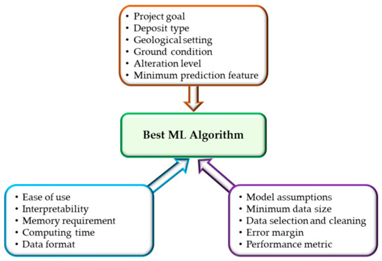
Figure 12.
Schematic of ML Rubric factors for mineral resource estimation.
It is important to indicate that a major drawback of ML applications is data limitation. The literature shows that most ML-based mineral resource estimation models were developed using composite values obtained from a few boreholes. Though these models produced satisfactory results, their performance can be improved with access to more data. The performance and accuracy of ML techniques, including deep learning, are highly dependent on a large and quality dataset that is partitioned appropriately into training, validation, and testing sets to ensure each set is a representative of the population [31]. It is well known that the functional capabilities of artificial intelligence and ML rest upon a sufficient dataset. However, what constitutes an adequate dataset size is not well defined, as the amount of data required can vary from one project to another. In this regard, studies such as Ganguli et al. [163] have provided recommendations to address ML application challenges peculiar to the mining industry. They recommended a comprehensive understanding of the modeling process before implementation and advised caution when using soft computing tools and software products [31]. Their recommendation also included the random data partition in three subsets (i.e., training, testing, and validation). Further, they suggested that the training subset should contain the highest and lowest values, and samples should be assigned to the training subset first, followed by validation and testing, during data grouping/segmentation. Additionally, the best data collection and processing protocols should be observed during model development to minimize error and ensure the dataset is good enough for its intended use.
6. Conclusions
Mineral resource estimation is a challenging task with enormous uncertainties, and considering the erratic nature of geological formations, results from such estimates are critical to all mining operations. Whether a mineral resource is classified as a reserve, ore, waste, and eventually a mine depends on the estimation outcome. Thus, the choice of the estimation method is key in the mineral resource estimation process. The selection of an unsuitable estimation method could defeat the purpose of an exploration program and may cause loss to capital expenditure. The common estimation methods in practice are in the geostatistical categories. These methods have been used to establish some of the most successful mining operations in the world, despite their weaknesses.
Recent developments in computer technologies allowed researchers to implement ML algorithms in mineral resource estimation. Results from such studies showed that ML algorithms are powerful tools for solving both linear and non-linear complex geological problems. These algorithms can model complex geological data, identify relationships, classify geological features, and detect geochemical anomalies with little human intervention. The most widely applied ML algorithms in this field are ANN, SVM, and RF. Given borehole data, the model can estimate ore grade values. However, despite their enormous potential in resource estimation, ML-based models also possess some inherent weaknesses such as overfitting, longer computational time, and smoothing effect.
These limitations can be addressed by combining them with other ML models and deep learning algorithms. The ML models could also be employed to augment existing estimation methods or perhaps integrated with traditional methods to form hybrid estimation methods. Furthermore, the mathematical complication associated with some of the ML algorithms, which could be a reason for their low implementation in the mining industry, can be rectified by incorporating them in existing resource estimation software as pre-trained models. Thus, the pre-trained models would make the implementation process much faster, easier, and user-friendly. Additionally, the resource engineer would not have to develop and train the algorithm from scratch but focus on retraining the pre-trained model with a new dataset. Future research can examine the application of ML techniques for grade estimation during a post-exploration stage (e.g., grade control and reconciliation), and they can also consider utilizing advanced ML methods, such as stochastic neural network and deep learning. Also, industry standards regarding ML applications can be developed to guide algorithm selection, build confidence in ML-based resource estimates, and promote industry-wide acceptance of ML techniques.
Author Contributions
Conceptualization, N.K.D.-D. and S.A.; writing—original draft preparation, N.K.D.-D.; writing—review and editing, S.A. All authors have read and agreed to the published version of the manuscript.
Funding
This research received no external funding.
Conflicts of Interest
The authors declare no conflict of interest.
References
- Coates, D.R. Mineral resources. In Geology and Society; Coates, D.R., Ed.; Springer: Boston, MA, USA, 1985; pp. 19–46. [Google Scholar]
- Dubiński, J. Sustainable Development of Mining Mineral Resources. J. Sustain. Min. 2013, 12, 1–6. [Google Scholar] [CrossRef]
- McMahon, G.; Moreira, S. The Contribution of the Mining Sector to Socioeconomic and Human Development. 2014. Available online: http://hdl.handle.net/10986/18660 (accessed on 20 May 2020).
- Löf, O.; Ericsson, M. Mining’s contribution to national economies. Eng. Min. J. 2018, 219, 48–56. [Google Scholar]
- Van Gosen, B.S.; Verplanck, P.L.; Long, K.R.; Gambogi, J.; Seal, R.R., II. The Rare-Earth Elements: Vital to Modern Technologies and Lifestyles; US Geological Survey: Reston, VA, USA, 2014. [Google Scholar]
- Henckens, M.L.C.M.; Biermann, F.H.B.; Driessen, P.P.J. Mineral resources governance: A call for the establishment of an International Competence Center on Mineral Resources Management. Resour. Conserv. Recycl. 2019, 141, 255–263. [Google Scholar] [CrossRef]
- Crowson, P.C.F. Mineral reserves and future minerals availability. Miner. Econ. 2011, 24, 1–6. [Google Scholar] [CrossRef]
- Zerzour, O.; Gadri, L.; Hadji, R.; Mebrouk, F.; Hamed, Y. Geostatistics-Based Method for Irregular Mineral Resource Estimation, in Ouenza Iron Mine, Northeastern Algeria. Geotech. Geol. Eng. 2021, 39, 3337–3346. [Google Scholar] [CrossRef]
- Tokoglu, M. Comparative Analysis of 3D Domain Modelling Alternatives: Implications for Mineral Resource Estimates; Colorado School of Mines: Golden, CO, USA, 2018. [Google Scholar]
- Abzalov, M.Z.; Bower, J. Geology of bauxite deposits and their resource estimation practices. Appl. Earth Sci. 2014, 123, 118–134. [Google Scholar] [CrossRef]
- Rossi, M.E.; Deutsch, C.V. Mineral Resource Estimation; Springer Science & Business Media: Berlin, Germany, 2014. [Google Scholar]
- Hartman, H.L.; Mutmansky, J.M. Introductory Mining Engineering, 2nd ed.; John Wiley & Sons: Hoboken, NJ, USA, 2002. [Google Scholar]
- Yunsel, T.Y. A practical application of geostatistical methods to quality and mineral reserve modelling of cement raw materials. J. S. Afr. Inst. Min. Metall. 2012, 112, 239–249. [Google Scholar]
- Shurygin, D.N.; Vlasenko, S.V.; Shutkova, V.V. Estimation of the Error in the Calculation of Mineral Reserves Taking into Account the Heterogeneity of the Geological Space; IOP Publishing: Bristol, UK, 2019; Volume 272, p. 22139. [Google Scholar]
- Wellmer, F.-W.; Dalheimer, M.; Wagner, M. Economic Evaluations in Exploration; Springer Science & Business Media: Berlin, Germany, 2007; ISBN 3540735593. [Google Scholar]
- Jones, O.; Lilford, E.; Chan, F. The Business of Mining: Mineral Project Valuation; CRC Press: Boca Raton, FL, USA, 2018; ISBN 0429622686. [Google Scholar]
- JORC. Australasian Code for Reporting of Exploration Results, Mineral Resources and Ore Reserves (The JORC Code). 2012. Available online: http://www.jorc.org/docs/JORC_code_2012.pdf (accessed on 20 May 2020).
- Dominy, S.C.; Noppé, M.A.; Annels, A.E. Errors and uncertainty in mineral resource and ore reserve estimation: The importance of getting it right. Explor. Min. Geol. 2002, 11, 77–98. [Google Scholar] [CrossRef]
- Abuntori, C.A.; Al-Hassan, S.; Mireku-Gyimah, D.; Ziggah, Y.Y. Evaluating the performance of Extreme Learning Machine technique for ore grade estimation. J. Sustain. Min. 2021, 20, 56–71. [Google Scholar] [CrossRef]
- Shirmard, H.; Farahbakhsh, E.; Muller, D.; Chandra, R. A review of machine learning in processing remote sensing data for mineral exploration. arXiv 2021, arXiv:2103.07678. [Google Scholar]
- Samson, M. Mineral Resource Estimates with Machine Learning and Geostatistics. Master’s Thesis, University of Alberta, Edmonton, AB, Canada, 2020. [Google Scholar]
- Cevik, S.I.; Ortiz, J.M. Machine Learning in the Mineral Resource Sector: An Overview. 2020. Available online: http://hdl.handle.net/1974/28545 (accessed on 20 January 2020).
- Jalloh, A.B.; Kyuro, S.; Jalloh, Y.; Barrie, A.K. Integrating artificial neural networks and geostatistics for optimum 3D geological block modeling in mineral reserve estimation: A case study. Int. J. Min. Sci. Technol. 2016, 26, 581–585. [Google Scholar] [CrossRef]
- Yasrebi, A.B.; Hezarkhani, A.; Afzal, P.; Karami, R.; Tehrani, M.E.; Borumandnia, A. Application of an ordinary kriging–artificial neural network for elemental distribution in Kahang porphyry deposit, Central Iran. Arab. J. Geosci. 2020, 13, 1–14. [Google Scholar] [CrossRef]
- Liakos, K.G.; Busato, P.; Moshou, D.; Pearson, S.; Bochtis, D. Machine learning in agriculture: A review. Sensors 2018, 18, 2674. [Google Scholar] [CrossRef]
- Ali, D.; Frimpong, S. Artificial intelligence, machine learning and process automation: Existing knowledge frontier and way forward for mining sector. Artif. Intell. Rev. 2020, 53, 6025–6042. [Google Scholar] [CrossRef]
- Hyder, Z.; Siau, K.; Nah, F. Artificial intelligence, machine learning, and autonomous technologies in mining industry. J. Database Manag. 2019, 30, 67–79. [Google Scholar] [CrossRef]
- Zhang, S.E.; Nwaila, G.T.; Tolmay, L.; Frimmel, H.E.; Bourdeau, J.E. Integration of machine learning algorithms with Gompertz Curves and Kriging to estimate resources in gold deposits. Nat. Resour. Res. 2021, 30, 39–56. [Google Scholar] [CrossRef]
- Jung, D.; Choi, Y. Systematic Review of machine learning applications in mining: Exploration, exploitation, and reclamation. Minerals 2021, 11, 148. [Google Scholar] [CrossRef]
- McCoy, J.T.; Auret, L. Machine learning applications in minerals processing: A review. Miner. Eng. 2019, 132, 95–109. [Google Scholar] [CrossRef]
- Dumakor-Dupey, N.K.; Arya, S.; Jha, A. Advances in blast-induced impact prediction—A review of machine learning applications. Minerals 2021, 11, 601. [Google Scholar] [CrossRef]
- Wee, B.V.; Banister, D. How to Write a Literature Review Paper? Transp. Rev. 2016, 36, 278–288. [Google Scholar] [CrossRef]
- Jalali, S.; Wohlin, C. Systematic literature studies: Database searches vs. backward snowballing. In Proceedings of the 2012 ACM-IEEE International Symposium on Empirical Software Engineering and Measurement, Lund, Sweden, 19–20 September 2012. [Google Scholar]
- Haldar, S.K. Mineral resource and ore reserve estimation. In Mineral Exploration; Elsevier: Amsterdam, The Netherlands, 2018; pp. 145–165. [Google Scholar]
- Afeni, T.B.; Akeju, V.O.; Aladejare, A.E. A comparative study of geometric and geostatistical methods for qualitative reserve estimation of limestone deposit. Geosci. Front. 2020, 12, 243–253. [Google Scholar] [CrossRef]
- Glacken, I.M.; Snowden, D.V. Mineral resource estimation. In Mineral Resource and Ore Reserve Estimation—The AusIMM Guide to Good Practice; Edwards, A.C., Ed.; The Australasian Institute of Mining and Metallurgy: Melbourne, Australia, 2001; pp. 189–198. [Google Scholar]
- Wu, X.; Zhou, Y. Reserve estimation using neural network techniques. Comput. Geosci. 1993, 19, 567–575. [Google Scholar] [CrossRef]
- Varouchakis, E.A. Geostatistics. In Spatiotemporal Analysis of Extreme Hydrological Events; Elsevier: Amsterdam, The Netherlands, 2018; ISBN 9780128116890. [Google Scholar]
- Gandhi, S.M.; Sarkar, B.C. Geostatistical resource/reserve estimation. In Essentials of Mineral Exploration and Evaluation; Elsevier: Amsterdam, The Netherlands, 2016; pp. 289–308. [Google Scholar]
- Shahbeik, S.; Afzal, P.; Moarefvand, P.; Qumarsy, M. Comparison between ordinary kriging (OK) and inverse distance weighted (IDW) based on estimation error case study: Dardevey iron ore deposit, NE Iran. Arab. J. Geosci. 2014, 7, 3693–3704. [Google Scholar] [CrossRef]
- Zarco-Perello, S.; Simões, N. Ordinary kriging vs inverse distance weighting: Spatial interpolation of the sessile community of Madagascar reef, Gulf of Mexico. PeerJ 2017, 5, e4078. [Google Scholar] [CrossRef]
- Osterholt, V.; Dimitrakopoulos, R. Simulation of orebody geology with multiple-point geostatistics-application at Yandi channel Iron ore deposit, WA, and implications for resource uncertainty. In Advances in Applied Strategic Mine Planning; Springer Science & Business Media: Berlin, Germany, 2018; pp. 335–352. [Google Scholar]
- Chen, Y.; Jiang, X.; Wang, Y.; Zhuang, D. Spatial characteristics of heavy metal pollution and the potential ecological risk of a typical mining area: A case study in China. Process Saf. Environ. Prot. 2018, 113, 204–219. [Google Scholar] [CrossRef]
- Dominy, S.C.; Hunt, S.P. Evaluation of gold deposits-Part 2: Results of a survey of estimation methodologies applied in the Eastern Goldfields of Western Australia. Trans. Inst. Min. Metall. Sect. B Appl. Earth Sci. 2001, 10, 167–175. [Google Scholar] [CrossRef]
- Yasrebi, A.B.; Afzal, P.; Wetherelt, A.; Foster, P.; Madani, N.; Javadi, A. Application of an inverse distance weighted anisotropic method (IDWAM) to estimate elemental distribution in Eastern Kahang Cu-Mo porphyry deposit, Central Iran. Int. J. Min. Miner. Eng. 2016, 7, 340. [Google Scholar] [CrossRef]
- Al-hassan, S.; David, A. Competitiveness of Inverse Distance Weighting Method for the Evaluation of Gold Resources in Fluvial Sedimentary Deposits: A Case Study. J. Geosci. Geomat. 2015, 3, 122–127. [Google Scholar] [CrossRef]
- Trong, V.D.; Bao, T.D.; Fomin, S.I. Ordinary kriging comparison and inverse distance weighting for quality assessment of Vietnam cement limestone deposits. In Proceedings of the International Multidisciplinary Scientific GeoConference Surveying Geology and Mining Ecology Management, Albena, Bulgaria, 29 June–5 July 2017. [Google Scholar] [CrossRef]
- Mallick, M.K.; Choudhary, B.S.; Budi, G. Geological reserve estimation of limestone deposit: A comparative study between ISDW and OK. Model. Meas. Control C 2020, 81, 72–77. [Google Scholar] [CrossRef]
- Ali Akbar, D. Reserve estimation of central part of Choghart north anomaly iron ore deposit through ordinary kriging method. Int. J. Min. Sci. Technol. 2012, 22, 573–577. [Google Scholar] [CrossRef]
- Daya, A.A.; Bejari, H. A comparative study between simple kriging and ordinary kriging for estimating and modeling the Cu concentration in Chehlkureh deposit, SE Iran. Arab. J. Geosci. 2015, 8, 6003–6020. [Google Scholar] [CrossRef]
- Yasrebi, J.; Saffari, M.; Fathi, H.; Karimian, N.; Moazallahi, M.; Gazni, R. Evaluation and comparison of ordinary kriging and inverse distance weighting methods for prediction of spatial variability of some chemical parameters. Res. J. Biol. Sci. 2009, 4, 93–102. [Google Scholar]
- Daya, A. Ordinary kriging for the estimation of vein type copper deposit: A case study of the Chelkureh, Iran. J. Min. Metall. A Min. 2015, 51, 1–14. [Google Scholar] [CrossRef]
- Hekmatnejad, A.; Emery, X.; Alipour-Shahsavari, M. Comparing linear and non-linear kriging for grade prediction and ore/waste classification in mineral deposits. Int. J. Min. Reclam. Environ. 2019, 33, 247–264. [Google Scholar] [CrossRef]
- Taboada, J.; Saavedra, Á.; Iglesias, C.; Giráldez, E. Estimating quartz reserves using compositional kriging. Abstr. Appl. Anal. 2013, 2013, 1–6. [Google Scholar] [CrossRef]
- Zuo, R. Machine Learning of mineralization-related geochemical anomalies: A Review of potential methods. Nat. Resour. Res. 2017, 26, 457–464. [Google Scholar] [CrossRef]
- Shanmuganathan, S. Artificial neural network modelling: An introduction. In Studies in Computational Intelligence; Springer Science & Business Media: Berlin, Germany, 2016; pp. 1–14. [Google Scholar]
- Prieto, A.; Prieto, B.; Ortigosa, E.M.; Ros, E.; Pelayo, F.; Ortega, J.; Rojas, I. Neural networks: An overview of early research, current frameworks and new challenges. Neurocomputing 2016, 214, 242–268. [Google Scholar] [CrossRef]
- Fung, C.C.; Iyer, V.; Brown, W.; Wong, K.W. Comparing the performance of different neural networks architectures for the prediction of mineral prospectivity. In Proceedings of the 2005 International Conference on Machine Learning and Cybernetics, Guangzhou, China, 18–21 August 2005; Volume 1, pp. 394–398. [Google Scholar]
- Leite, E.P.; de Souza Filho, C.R. Artificial neural networks applied to mineral potential mapping for copper-gold mineralizations in the Carajás Mineral Province, Brazil. Geophys. Prospect. 2009, 57, 1049–1065. [Google Scholar] [CrossRef]
- Rigol-Sanchez, J.P.; Chica-Olmo, M.; Abarca-Hernandez, F. Artificial neural networks as a tool for mineral potential mapping with GIS. Int. J. Remote Sens. 2003, 24, 1151–1156. [Google Scholar] [CrossRef]
- Lee, S.; Oh, H.-J. Application of artificial neural network for mineral potential mapping. In Artificial Neural Networks-Application; BoD–Books on Demand: Norderstedt, Germany, 2011. [Google Scholar]
- Oh, H.J.; Lee, S. Application of artificial neural network for gold-silver deposits potential mapping: A case study of Korea. Nat. Resour. Res. 2010, 19, 103–124. [Google Scholar] [CrossRef]
- Singer, D.A.; Kouda, R. Application of a feedforward neural network in the search for kuroko deposits in the hokuroku district, Japan. Math. Geol. 1996, 28, 1017–1023. [Google Scholar] [CrossRef]
- Harris, D.V.; Pan, G. Mineral favorability mapping: A comparison of artificial neural networks, logistic regression, and discriminant analysis. Nat. Resour. Res. 1999, 8, 93–109. [Google Scholar] [CrossRef]
- Nie, W.; Fang, J.; Wen, S.; Feng, Q.; He, Y.; Yang, X. Estimation and improvement of recovery of low grade copper oxide using sulfide activation flotation method based on GA–BPNN. Processes 2021, 9, 583. [Google Scholar] [CrossRef]
- Al-Alawi, S.M.; Tawo, E.E. Application of Artificial Neural Networks in Mineral Resource Evaluation. J. King Saud Univ. Eng. Sci. 1998, 10, 127–138. [Google Scholar] [CrossRef]
- Yama, B.R.; Lineberry, G.T. Artificial neural network application for a predictive task in mining. Min. Eng. 1999, 51, 59–64. [Google Scholar]
- Koike, K.; Matsuda, S.; Suzuki, T.; Ohmi, M. Neural network-based estimation of principal metal contents in the Hokuroku District, Northern Japan, for exploring Kuroko-type deposits. Nat. Resour. Res. 2002, 11, 135–156. [Google Scholar] [CrossRef]
- Tahmasebi, P.; Hezarkhani, A. Application of adaptive neuro-fuzzy inference system for grade estimation; case study, sarcheshmeh porphyry copper deposit, Kerman, Iran. Aust. J. Basic Appl. Sci. 2010, 4, 408–420. [Google Scholar]
- Tahmasebi, P.; Hezarkhani, A. Application of a Modular Feedforward Neural Network for Grade Estimation. Nat. Resour. Res. 2011, 20, 25–32. [Google Scholar] [CrossRef]
- Matías, J.M.; Vaamonde, A.; Taboada, J.; González-Manteiga, W. Comparison of kriging and neural networks with application to the exploitation of a slate mine. Math. Geol. 2004, 36, 463–486. [Google Scholar] [CrossRef]
- Chatterjee, S.; Bhattacherjee, A.; Samanta, B.; Pal, S.K. Ore grade estimation of a limestone deposit in India using an artificial neural network. Appl. GIS 2006, 2, 3.1–3.20. [Google Scholar] [CrossRef]
- Kaplan, U.E.; Topal, E. A new ore grade estimation using combine machine learning algorithms. Minerals 2020, 10, 847. [Google Scholar] [CrossRef]
- Tutmez, B. An uncertainty oriented fuzzy methodology for grade estimation. Comput. Geosci. 2007, 33, 280–288. [Google Scholar] [CrossRef]
- Tutmez, B.; Tercan, A.E.; Kaymak, U. Fuzzy modeling for reserve estimation based on spatial variability. Math. Geol. 2007, 39, 87–111. [Google Scholar] [CrossRef]
- Tutmez, B. Use of hybrid intelligent computing in mineral resources evaluation. Appl. Soft Comput. J. 2009, 9, 1023–1028. [Google Scholar] [CrossRef]
- Tahmasebi, P.; Hezarkhani, A.; Mortazavi, M. Application of discriminant analysis for alteration separation; Sungun copper deposit, East Azerbaijan, Iran. Aust. J. Basic Appl. Sci. 2010, 6, 565. [Google Scholar]
- Tahmasebi, P.; Hezarkhani, A. A hybrid neural networks-fuzzy logic-genetic algorithm for grade estimation. Comput. Geosci. 2012, 42, 18–27. [Google Scholar] [CrossRef]
- Li, X.-L.; Xie, Y.-L.; Guo, Q.-J.; Li, L.-H. Adaptive ore grade estimation method for the mineral deposit evaluation. Math. Comput. Model. 2010, 52, 1947–1956. [Google Scholar] [CrossRef]
- Singh, R.K.; Ray, D.; Sarkar, B.C. Recurrent neural network approach to mineral deposit modelling. In Proceedings of the Proceedings of the 4th IEEE International Conference on Recent Advances in Information Technology, Dhanbad, India, 15–17 March 2018. [Google Scholar]
- Huang, Y.; Wänstedt, S. Application of Kalman learning algorithm multilayer neural network to estimates of ore grades. Int. J. Surf. Min. Reclam. Environ. 1998, 12, 19–27. [Google Scholar] [CrossRef]
- Jafrasteh, B.; Fathianpour, N. A hybrid simultaneous perturbation artificial bee colony and back-propagation algorithm for training a local linear radial basis neural network on ore grade estimation. Neurocomputing 2017, 235, 217–227. [Google Scholar] [CrossRef]
- Samanta, B. Radial basis function network for ore grade estimation. Nat. Resour. Res. 2010, 19, 91–102. [Google Scholar] [CrossRef]
- Samanta, B.; Bandopadhyay, S. Construction of a radial basis function network using an evolutionary algorithm for grade estimation in a placer gold deposit. Comput. Geosci. 2009, 35, 1592–1602. [Google Scholar] [CrossRef]
- Vapnik, V.N. The Nature of Statistical Learning Theory; Springer Science & Business Media: Berlin, Germany, 2013. [Google Scholar]
- Chatterjee, S.; Bandopadhyay, S. Goodnews Bay Platinum resource estimation using least squares support vector regression with selection of input space dimension and hyperparameters. Nat. Resour. Res. 2011, 20, 117–129. [Google Scholar] [CrossRef]
- Li, X.; Li, L.; Zhang, B.; Guo, Q. Hybrid self-adaptive learning based particle swarm optimization and support vector regression model for grade estimation. Neurocomputing 2013, 118, 179–190. [Google Scholar] [CrossRef]
- Zuo, R.; Carranza, E.J.M. Support vector machine: A tool for mapping mineral prospectivity. Comput. Geosci. 2011, 37, 1967–1975. [Google Scholar] [CrossRef]
- Rodriguez-Galiano, V.; Sanchez-Castillo, M.; Chica-Olmo, M.; Chica-Rivas, M. Machine learning predictive models for mineral prospectivity: An evaluation of neural networks, random forest, regression trees and support vector machines. Ore Geol. Rev. 2015, 71, 804–818. [Google Scholar] [CrossRef]
- Geranian, H.; Tabatabaei, S.H.; Asadi, H.H.; Carranza, E.J.M. Application of discriminant analysis and support vector machine in mapping gold potential areas for further drilling in the Sari-Gunay gold deposit, NW Iran. Nat. Resour. Res. 2016, 25, 145–159. [Google Scholar] [CrossRef]
- Mahvash Mohammadi, N.; Hezarkhani, A. Application of support vector machine for the separation of mineralised zones in the Takht-e-Gonbad porphyry deposit, SE Iran. J. Afr. Earth Sci. 2018, 143, 301–308. [Google Scholar] [CrossRef]
- Ghezelbash, R.; Maghsoudi, A.; Carranza, E.J.M. Performance evaluation of RBF- and SVM-based machine learning algorithms for predictive mineral prospectivity modeling: Integration of S-A multifractal model and mineralization controls. Earth Sci. Inform. 2019, 12, 277–293. [Google Scholar] [CrossRef]
- Abbaszadeh, M.; Hezarkhani, A.; Soltani-Mohammadi, S. Proposing drilling locations based on the 3D modeling results of fluid inclusion data using the support vector regression method. J. Geochem. Explor. 2016, 165, 23–34. [Google Scholar] [CrossRef]
- Abbaszadeh, M.; Hezarkhani, A.; Soltani-Mohammadi, S. Classification of alteration zones based on whole-rock geochemical data using support vector machine. J. Geol. Soc. India 2015, 85, 500–508. [Google Scholar] [CrossRef]
- Abbaszadeh, M.; Hezarkhani, A.; Soltani-Mohammadi, S. An SVM-based machine learning method for the separation of alteration zones in Sungun porphyry copper deposit. Geochemistry 2013, 73, 545–554. [Google Scholar] [CrossRef]
- Taboada, J.; Matías, J.M.; Ordóñez, C.; García, P.J. Creating a quality map of a slate deposit using support vector machines. J. Comput. Appl. Math. 2007, 204, 84–94. [Google Scholar] [CrossRef]
- Das Goswami, A.; Mishra, M.K.; Patra, D. Adapting pattern recognition approach for uncertainty assessment in the geologic resource estimation for Indian iron ore mines. In Proceedings of the International Conference on Signal Processing, Communication, Power and Embedded System, Sankt Goar, Germany, 23–25 May 2016. [Google Scholar]
- Zhang, X.; Song, S.; Li, J.; Cheng, W. Robust LS-SVM regression for ore grade estimation in a seafloor hydrothermal sulphide deposit. Acta Oceanol. Sin. 2013, 32, 16–25. [Google Scholar] [CrossRef]
- Zhang, Y.; Song, S.; You, K.; Zhang, X.; Wu, C. Relevance vector machines using weighted expected squared distance for ore grade estimation with incomplete data. Int. J. Mach. Learn. Cybern. 2017, 8, 1655–1666. [Google Scholar] [CrossRef]
- Tipping, M.E. The relevance vector machine. In Advances in Neural Information Processing Systems; MIT Press: Cambridge, MA, USA, 2001. [Google Scholar]
- Breiman, L. Random Forests. Mach. Learn. 2001, 45, 5–32. [Google Scholar] [CrossRef]
- Zhang, L.; Suganthan, P.N. Random Forests with ensemble of feature spaces. Pattern Recognit. 2014, 47, 3429–3437. [Google Scholar] [CrossRef]
- Pal, M. Random forest classifier for remote sensing classification. Int. J. Remote Sens. 2005, 26, 217–222. [Google Scholar] [CrossRef]
- Rodriguez-Galiano, V.F.; Ghimire, B.; Rogan, J.; Chica-Olmo, M.; Rigol-Sanchez, J.P. An assessment of the effectiveness of a random forest classifier for land-cover classification. ISPRS J. Photogramm. Remote Sens. 2012, 67, 93–104. [Google Scholar] [CrossRef]
- Ao, Y.; Li, H.; Zhu, L.; Ali, S.; Yang, Z. The linear random forest algorithm and its advantages in machine learning assisted logging regression modeling. J. Pet. Sci. Eng. 2019, 174, 776–789. [Google Scholar] [CrossRef]
- Belgiu, M.; Drăgu, L. Random forest in remote sensing: A review of applications and future directions. ISPRS J. Photogramm. Remote Sens. 2016, 114, 24–31. [Google Scholar] [CrossRef]
- Naghibi, S.A.; Pourghasemi, H.R.; Dixon, B. GIS-based groundwater potential mapping using boosted regression tree, classification and regression tree, and random forest machine learning models in Iran. Environ. Monit. Assess. 2016, 188, 1–27. [Google Scholar] [CrossRef]
- Baudron, P.; Alonso-Sarría, F.; García-Aróstegui, J.L.; Cánovas-García, F.; Martínez-Vicente, D.; Moreno-Brotóns, J. Identifying the origin of groundwater samples in a multi-layer aquifer system with Random Forest classification. J. Hydrol. 2013, 499, 303–315. [Google Scholar] [CrossRef]
- McKay, G.; Harris, J.R. Comparison of the data-driven random forests model and a knowledge-driven method for mineral prospectivity mapping: A case study for gold deposits around the Huritz Group and Nueltin Suite, Nunavut, Canada. Nat. Resour. Res. 2016, 25, 125–143. [Google Scholar] [CrossRef]
- Jafrasteh, B.; Fathianpour, N.; Suárez, A. Comparison of machine learning methods for copper ore grade estimation. Comput. Geosci. 2018, 22, 1371–1388. [Google Scholar] [CrossRef]
- Sheng, L.; Zhang, T.; Niu, G.; Wang, K.; Tang, H.; Duan, Y.; Li, H. Classification of iron ores by laser-induced breakdown spectroscopy (LIBS) combined with random forest (RF). J. Anal. At. Spectrom. 2015, 30, 453–458. [Google Scholar] [CrossRef]
- O’Brien, J.J.; Spry, P.G.; Nettleton, D.; Xu, R.; Teale, G.S. Using random forests to distinguish gahnite compositions as an exploration guide to broken hill-type Pb-Zn-Ag deposits in the broken hill domain, Australia. J. Geochem. Explor. 2014, 149, 74–86. [Google Scholar] [CrossRef]
- Schnitzler, N.; Ross, P.S.; Gloaguen, E. Using machine learning to estimate a key missing geochemical variable in mining exploration: Application of the Random Forest algorithm to multi-sensor core logging data. J. Geochem. Explor. 2019, 205, 106344. [Google Scholar] [CrossRef]
- Matin, S.S.; Chelgani, S.C. Estimation of coal gross calorific value based on various analyses by random forest method. Fuel 2016, 177, 274–278. [Google Scholar] [CrossRef]
- Seeger, M. Gaussian processes for machine learning. Int. J. Neural Syst. 2004, 14, 69–106. [Google Scholar] [CrossRef] [PubMed]
- Rasmussen, C.E.; Williams, C.K.I. Gaussian Processes for Machine Learning. 2006. Available online: http://www.gaussianprocess.org/gpml/chapters/RW.pdf (accessed on 20 May 2020).
- Chen, F.; Chen, S.; Peng, G. Using Sequential Gaussian Simulation to Assess Geochemical Anomaly Areas of Lead Element; Springer: Berlin, Germany, 2013. [Google Scholar]
- Wang, J.; Zuo, R. Identification of geochemical anomalies through combined sequential Gaussian simulation and grid-based local singularity analysis. Comput. Geosci. 2018, 118, 52–64. [Google Scholar] [CrossRef]
- Soltani, F.; Afzal, P.; Asghari, O. Delineation of alteration zones based on Sequential Gaussian Simulation and concentration-volume fractal modeling in the hypogene zone of Sungun copper deposit, NW Iran. J. Geochem. Explor. 2014, 140, 64–76. [Google Scholar] [CrossRef]
- Afzal, P.; Madani, N.; Shahbeik, S.; Yasrebi, A.B. Multi-Gaussian kriging: A practice to enhance delineation of mineralized zones by Concentration-Volume fractal model in Dardevey iron ore deposit, SE Iran. J. Geochem. Explor. 2015, 158, 10–21. [Google Scholar] [CrossRef]
- Bazdar, H.; Fattahi, H.; Ghadimi, F. Hybrid ANN with invasive weed optimization algorithm, a new technique for prediction of gold and silver in Zarshuran gold deposit, Iran. Q. J. Tethys 2015, 3, 273–285. [Google Scholar]
- Mahmoudabadi, H.; Izadi, M.; Menhaj, M.B. A hybrid method for grade estimation using genetic algorithm and neural networks. Comput. Geosci. 2009, 13, 91–101. [Google Scholar] [CrossRef]
- Yu, S.; Zhu, K.; He, Y. A hybrid intelligent optimization method for multiple metal grades optimization. Neural Comput. Appl. 2012, 21, 1391–1402. [Google Scholar] [CrossRef]
- Chatterjee, S.; Bhattacherjee, A. Genetic algorithms for feature selection of image analysis-based quality monitoring model: An application to an iron mine. Eng. Appl. Artif. Intell. 2011, 24, 786–795. [Google Scholar] [CrossRef]
- Patel, A.K.; Chatterjee, S.; Gorai, A.K. Development of a machine vision system using the support vector machine regression (SVR) algorithm for the online prediction of iron ore grades. Earth Sci. Inform. 2019, 12, 197–210. [Google Scholar] [CrossRef]
- Patel, A.K.; Chatterjee, S. Computer vision-based limestone rock-type classification using probabilistic neural network. Geosci. Front. 2016, 7, 53–60. [Google Scholar] [CrossRef]
- Perez, C.A.; Estévez, P.A.; Vera, P.A.; Castillo, L.E.; Aravena, C.M.; Schulz, D.A.; Medina, L.E. Ore grade estimation by feature selection and voting using boundary detection in digital image analysis. Int. J. Miner. Process. 2011, 101, 28–36. [Google Scholar] [CrossRef]
- Zhang, Z.; Yang, J.; Wang, Y.; Dou, D.; Xia, W. Ash content prediction of coarse coal by image analysis and GA-SVM. Powder Technol. 2014, 268, 429–435. [Google Scholar] [CrossRef]
- Kanevski, M. Machine Learning for Spatial Environmental Data: Theory, Applications, and Software; EPFL Press: Lausanne, Switzerland, 2009. [Google Scholar]
- Li, J.; Heap, A.D.; Potter, A.; Daniell, J.J. Application of machine learning methods to spatial interpolation of environmental variables. Environ. Model. Softw. 2011, 26, 1647–1659. [Google Scholar] [CrossRef]
- Lary, D.J.; Alavi, A.H.; Gandomi, A.H.; Walker, A.L. Machine learning in geosciences and remote sensing. Geosci. Front. 2016, 7, 3–10. [Google Scholar] [CrossRef]
- Karami, R.; Afzal, P. Estimation of elemental distributions by combining artificial neural network and Inverse Distance Weighted (IDW) based on lithogeochemical data in Kahang porphry deposit, Central Iran. Univers. J. Geosci. 2015, 3, 59–65. [Google Scholar] [CrossRef]
- Dutta, S.; Bandopadhyay, S.; Ganguli, R.; Misra, D. Machine learning algorithms and their application to ore reserve estimation of sparse and imprecise data. J. Intell. Learn. Syst. Appl. 2010, 2, 86. [Google Scholar] [CrossRef]
- Das Goswami, A.; Mishra, M.K.; Patra, D. Investigation of general regression neural network architecture for grade estimation of an Indian iron ore deposit. Arab. J. Geosci. 2017, 10. [Google Scholar] [CrossRef]
- Lishchuk, V.; Lund, C.; Ghorbani, Y. Evaluation and comparison of different machine-learning methods to integrate sparse process data into a spatial model in geometallurgy. Miner. Eng. 2019, 134, 156–165. [Google Scholar] [CrossRef]
- Ishikawa, S.T.; Gulick, V.C. An automated mineral classifier using Raman spectra. Comput. Geosci. 2013, 54, 259–268. [Google Scholar] [CrossRef]
- Fouedjio, F.; Klump, J. Exploring prediction uncertainty of spatial data in geostatistical and machine learning approaches. Environ. Earth Sci. 2019, 78, 38. [Google Scholar] [CrossRef]
- Nwaila, G.T.; Zhang, S.E.; Frimmel, H.E.; Manzi, M.S.D.; Dohm, C.; Durrheim, R.J.; Burnett, M.; Tolmay, L. Local and target exploration of conglomerate-hosted gold deposits using machine learning algorithms: A case study of the Witwatersrand gold ores, South Africa. Nat. Resour. Res. 2020, 29, 135–159. [Google Scholar] [CrossRef]
- Caté, A.; Perozzi, L.; Gloaguen, E.; Blouin, M. Machine learning as a tool for geologists. Lead. Edge 2017, 36, 215–219. [Google Scholar] [CrossRef]
- Chen, L.; Ren, C.; Li, L.; Wang, Y.; Zhang, B.; Wang, Z.; Li, L. A comparative assessment of geostatistical, machine learning, and hybrid approaches for mapping topsoil organic carbon content. ISPRS Int. J. Geo-Inf. 2019, 8, 174. [Google Scholar] [CrossRef]
- Jafrasteh, B.; Fathianpour, N.; Suárez, A. Advanced Machine Learning Methods for Copper Ore Grade Estimation; European Association of Geoscientists & Engineers: Houten, The Netherlands, 2016. [Google Scholar]
- Afeni, T.B.; Lawal, A.I.; Adeyemi, R.A. Re-examination of Itakpe iron ore deposit for reserve estimation using geostatistics and artificial neural network techniques. Arab. J. Geosci. 2020, 13, 657. [Google Scholar] [CrossRef]
- Kapageridis, I.K. Input space configuration effects in neural network-based grade estimation. Comput. Geosci. 2005, 31, 704–717. [Google Scholar] [CrossRef]
- Erdogan Erten, G.; Yavuz, M.; Deutsch, C.V. Grade estimation by a machine learning model using coordinate rotations. Appl. Earth Sci. 2021, 130, 57–66. [Google Scholar] [CrossRef]
- Chatterjee, S.; Bandopadhyay, S.; Machuca, D. Ore grade prediction using a genetic algorithm and clustering Based ensemble neural network model. Math. Geosci. 2010, 42, 309–326. [Google Scholar] [CrossRef]
- Zhou, Z.H. Ensemble Methods: Foundations and Algorithms; CRC Press: Boca Raton, FL, USA, 2012; ISBN 9781439830055. [Google Scholar]
- Li, Y.; Gao, J.; Li, Q.; Fan, W. Ensemble learning. In Data Classification: Algorithms and Applications; CRC Press: Boca Raton, FL, USA, 2014; ISBN 9781466586758. [Google Scholar]
- Chatterjee, S.; Bandopadhyay, S.; Rai, P. Genetic algorithm-based neural network learning parameter selection for ore grade evaluation of limestone deposit. Min. Technol. 2008, 117, 178–190. [Google Scholar] [CrossRef]
- Tahmasebi, P.; Hezarkhani, A. Application of Optimized Neural Network by Genetic Algorithm, IAMG09; Stanford University: Stanford, CA, USA, 2009. [Google Scholar]
- Samanta, B.; Bandopadhyay, S.; Ganguli, R. Data segmentation and genetic algorithms for sparse data division in Nome placer gold grade estimation using neural network and geostatistics. Explor. Min. Geol. 2002, 11, 69–76. [Google Scholar] [CrossRef]
- Tang, Y.; Salakhutdinov, R. Learning stochastic feedforward neural networks. In Proceedings of the Advances in Neural Information Processing Systems, Lake Tahoe, NV, USA, 5–8 December 2013. [Google Scholar]
- Ling, H.; Samarasinghe, S.; Kulasiri, D. Stochastic neural networks for modelling random processes from observed data. In Artificial Neural Network Modelling; Springer: Berlin, Germany, 2016. [Google Scholar]
- Kapageridis, I.K.; Denby, B.; Hunter, G. Integration of a neural ore grade estimation tool in a 3D resource modeling package. In Proceedings of the International Joint Conference on Neural Networks, Washington, DC, USA, 10–16 July 1999. [Google Scholar]
- Kapageridis, I.K. Application of Artificial Neural Network Systems to Grade Estimation from Exploration Data. Ph.D. Thesis, University of Nottingham, Nottingham, UK, 1999. [Google Scholar]
- Žliobaitė, I.; Pechenizkiy, M.; Gama, J. An overview of concept drift applications. Big Data Anal. New Algorithms New Soc. 2016, 16, 91–114. [Google Scholar]
- Žliobaitė, I. Learning under concept drift: An overview. arXiv 2010, arXiv:1010.4784. [Google Scholar]
- Zhukov, A.V.; Sidorov, D.N.; Foley, A.M. Random Forest Based Approach for Concept Drift Handling; Springer: Berlin, Germany, 2016; pp. 69–77. [Google Scholar]
- Zenisek, J.; Holzinger, F.; Affenzeller, M. Machine learning based concept drift detection for predictive maintenance. Comput. Ind. Eng. 2019, 137, 106031. [Google Scholar] [CrossRef]
- Namitha, K. Concept drift detection in data stream clustering and its application on weather data. Int. J. Agric. Environ. Inf. Syst. 2020, 11, 67–85. [Google Scholar] [CrossRef]
- Fdez-Riverola, F.; Iglesias, E.L.; Díaz, F.; Méndez, J.R.; Corchado, J.M. Applying lazy learning algorithms to tackle concept drift in spam filtering. Expert Syst. Appl. 2007, 33, 36–48. [Google Scholar] [CrossRef]
- Sayadi, A.R.; Tavassoli, S.M.M.; Monjezi, M.; Rezaei, M. Application of neural networks to predict net present value in mining projects. Arab. J. Geosci. 2014, 7, 1067–1072. [Google Scholar] [CrossRef]
- Zhang, H.; Nguyen, H.; Bui, X.N.; Nguyen-Thoi, T.; Bui, T.T.; Nguyen, N.; Vu, D.A.; Mahesh, V.; Moayedi, H. Developing a novel artificial intelligence model to estimate the capital cost of mining projects using deep neural network-based ant colony optimization algorithm. Resour. Policy 2020, 66, 101604. [Google Scholar] [CrossRef]
- Ganguli, R.; Dagdelen, K.; Grygiel, E. System engineering. In SME Mining Engineering Handbook; Darling, P., Ed.; SME: Englewood, CO, USA, 2011; pp. 839–853. [Google Scholar]
Publisher’s Note: MDPI stays neutral with regard to jurisdictional claims in published maps and institutional affiliations. |
© 2021 by the authors. Licensee MDPI, Basel, Switzerland. This article is an open access article distributed under the terms and conditions of the Creative Commons Attribution (CC BY) license (https://creativecommons.org/licenses/by/4.0/).