Article

A Compressed Sensing Recovery Algorithm Based on Support Set Selection

1
School of Electrical and Information Engineering, Tianjin University, Tianjin 300072, China
2
College of Physics, Guizhou University, Guiyang 550025, China
*
Author to whom correspondence should be addressed.
Electronics 2021, 10(13), 1544; https://doi.org/10.3390/electronics10131544
Submission received: 16 May 2021 / Revised: 10 June 2021 / Accepted: 21 June 2021 / Published: 25 June 2021
(This article belongs to the Section Industrial Electronics)

Abstract

:
The theory of compressed sensing (CS) has shown tremendous potential in many fields, especially in the signal processing area, due to its utility in recovering unknown signals with far lower sampling rates than the Nyquist frequency. In this paper, we present a novel, optimized recovery algorithm named supp-BPDN. The proposed algorithm executes a step of selecting and recording the support set of original signals before using the traditional recovery algorithm mostly used in signal processing called basis pursuit denoising (BPDN). We proved mathematically that even in a noise-affected CS system, the probability of selecting the support set of signals still approaches 1, which means supp-BPDN can maintain good performance in systems in which noise exists. Recovery results are demonstrated to verify the effectiveness and superiority of supp-BPDN. Besides, we set up a photonic-enabled CS system realizing the reconstruction of a two-tone signal with a peak frequency of 350 MHz through a 200 MHz analog-to-digital converter (ADC) and a signal with a peak frequency of 1 GHz by a 500 MHz ADC. Similarly, supp-BPDN showed better reconstruction results than BPDN.

1. Introduction

Compressed sensing (CS) is a theory that describes an unknown high-dimensional signal with few non-zero components that can be recovered from extremely incomplete information, which could reduce data redundancy to a considerable extent. Since CS theory was conceived [1,2], it attracted great attention all over the world for its applicability to many fields, such as signal processing, radar systems [3], imaging [4,5], optical microscopy [6], direction of arrival (DOA) [7], and cognitive radio (CR) [8]. In the signal processing area in particular, the rapid development of communication technologies, the utilization of high-speed computers, and high-frequency or ultrawide band signals have caused explosive growth of data, along with serious challenges to digital devices such as the analog-to-digital converter (ADC) using the Nyquist sampling theory [9,10], which limits the sampling rate to twice or above the highest frequency of signals. Nevertheless, CS systems can greatly overcome above difficulties.
CS systems are composed of two parts: measurement and reconstruction. In the former part, signals are compressively and randomly measured by the measurement matrix (MM), which usually consists of groups of pseudo random bit sequence (PRBS) in communication systems, by mixing the signal with PRBS with mixers or modulators. In other words, high-dimensional signals are projected randomly and linearly to a much lower-dimensional space, making it possible to reduce the requirement of sampling rate. Many works have been done in this area during the past decades and have made great progress. In the very beginning, an CS system was implemented in electronic systems called the random demodulator (RD) [11,12]. In the RD, a microwave signal is directly mixed with PRBS via a mixer and accumulated by an accumulator or a low-pass filter (LPF); this is done in awareness of the sampling rate being exponentially lower than the Nyquist rate, which was pioneering at that time. Recent years, researchers turned their eyes to photonics-enabled CS systems due to the advantages of low loss, large bandwidth, and high speed offered by photonics [13,14,15,16,17,18,19,20,21,22,23,24]. In [13], a CS system in a photonic link was demonstrated for the first time, which successfully recovered a 1 GHz harmonic signal with 500 MS/s sampling rate. Afterwards the researcher introduced the time stretch technique to broaden the pulse width in order to lower the sampling rate even further, and realized the integration process by compressing the optical pulses before photodiode (PD) [17,21,22]. Under this scheme, signals spanning from 900 MHz to 14.76 GHz can be recovered by a 500 MHz ADC. In contrast to the above systems using optical pulses generated by lasers, a CS system can be accomplished by using a broadband light source instead [23]. Moreover, [24] mixed a signal with PRBS using spatial light modulator (SLM), rather than Mach–Zehnder modulator (MZM), as in the above schemes. In the signal reconstruction part, until now recovery algorithms have mostly been divided into three categories, which are convex optimization methods [25,26], greedy algorithms [27,28,29,30,31,32], and Bayesian compressive sensing (BCS) approaches [33,34,35]. Convex optimization methods are basically composed of basis pursuit (BP), BPDN, and extended algorithms, and explicit details are discussed in the following sections. The main form of greedy algorithms is iteration and residual updating. As a fundamental method in greedy algorithms, the matching pursuit (MP) method chooses an optimal value, and only columns related to the chosen value in MM will be updated in the measurements during each iteration, whereas in the orthogonal matching pursuit (OMP) method, residuals are updated and iterated in the global range. Additionally, optimized algorithms have been formulated that choose more than one value each time [29], have dynamic selecting numbers [30], have different application situations [31,32] and so on. Moreover, based on the Bayesian formalism, BCS algorithm came about and is a promising research direction as well. Differently from convex optimization methods and greedy algorithms, which are non-adaptive, BCS provides a framework for sequential adaptive sensing, i.e., automatically adjusting the recovery process. Besides, under BCS, other observations such as posterior density function, confidence, and uncertainty estimation are obtained. Among these algorithms, the greedy algorithm is fastest and easiest; the convex optimization algorithm is the most accurate and is suitable for large signals. Additionally, although BCS acquires the smallest reconstruction errors, its complexity is a barrier. Thus, in practical CS communication systems, convex optimization algorithms such as BPDN are more popular choices.
In this paper, based on support set selection, we present a novel algorithm which has better reconstruction performance than that of the BPDN algorithm. In our optimized algorithm, finding where the non-zero components are is the first thing to do, and it is named the supp-BPDN algorithm. We proved that not only in ideal CS systems, but also in the more common situation with noise influence, the support set of the original signal can be found from the maximum value of an inner product of measurements and a column vector of MM at high probability.
We combined the support set selection and BPDN innovatively. Additionally, supp-BPDN recovers signals by relying on BPDN rather than the least squares method; thus, a more accurate reconstruction can be obtained. Furthermore, differently from the support set selection of MP and relative algorithms, it is unnecessary to update measurements and get residuals during each iteration during the mathematical analysis. Overall, supp-BPDN has a better performance in recovering signals.
The organization of the paper is as follows. Section 1 is the the background and introduction of CS theory. Section 2 outlines the principle of CS theory and briefly analyzes the convex optimization algorithm. In Section 3, supp-BPDN is put forward and the principle of it is analyzed in detail. Section 4 demonstrates a series of numerical simulations to support our mathematical proof and show the superiority of supp-BPDN. In the following section, a CS system is proposed and simulated results are presented, verifying the effectiveness of supp-BPDN. Conclusions are drawn in the final section.

2. Principles

2.1. CS Theory

Consider an unknown vector x R N of N-length, x only containing k non-zero elements, and k N , the index set of these non-zero elements is defined as the support set supp x , which is
supp x = i N ,   x i 0 ,
where N = 1 ,   2 ,   ,   N is the index set of all elements in x . In other words, N is all the subscripts of elements in x . Equation (1) means the other N k components are totally equal to zero. It is the strict definition of “sparsity”, which is the precondition of CS theory. However, there are few signals totally meeting the requirement that other components are all zero. To expand the application range of CS, luckily, the condition can be relaxed. At this time x is called “compressible.” The N k components in compressible signal are really small values, not strictly equal to zero. The sparsity or compressibility of a signal is the premise of CS.
Under such conditions, CS states that
y = Φ x ,
in which y R M is the measurement vector, composed of measurements. Besides, Φ R M × N is the MM, and they hold the relation that k < M N . MM must obey the restricted isometry property (RIP) [36], which defines the restricted isometry constant (RIC) to be the smallest value δ k that makes
1 δ k x 2 2 Φ x 2 2 1 + δ k x 2 2
hold for all k-sparse signals. RIP guarantees that the mapping relationship from x to y is unique and determined; i.e., different k-sparse signals cannot be mapped to the same y through Φ which obeys RIP.
The process of signal reconstruction is actually solving Equation (2), and the original unknown signal can be recovered by reconstruction algorithms. Besides, it is worth noticing that as long as the signal is sparse in any domain, such as the frequency domain or wavelet domain, the signal can be regarded as sparse and recovered as well. In a mathematical expression, it is
s i = j = 1 N ψ i j x j ( i , j = 1 , 2 , , N ) ,
or in a matrix expression, s = Ψ x , among which Ψ R N is the orthogonal transformation basis. x is still the sparse vector. It is known that when M is not very small, Θ = Φ Ψ also abides by the RIP at high probability according to the universality of CS [37,38], making the application range of CS much wider as well. Therefore, although s is not sparse, it can be recovered in CS system. It is more suitable for communication systems when Ψ stands for the Fourier transform matrix.

2.2. Problem Statement

We mean to outline signal reconstruction in communication systems under CS theory. The original unknown signal, denoted as s , is the sum of different cosine signals, and obviously it is sparse in frequency domain. In consideration of noise in actual systems, such as shot noise and thermal noise in PD, and quantization noise in ADC, from Equation (2) and Equation (4), the model of CS-enabled communication system is
y noise = Θ x + n = Φ s + n ,
where n is additive noise, and n R M . In this specific situation, MM is usually used as the matrix composed of M groups of PRBS consisting of 0 and 1, denoted as r 1 until r M . Hence, the detailed expression of MM is
Φ = r 1 r 2 r M = r 11   r 12     r 1 N . . . r M 1   r M 2     r M N = φ 1   φ 2     φ N ,
in which φ i = r 1 i   r 2 i     r M i T is the i th column vector of Φ .

2.3. Convex Optimization Recovery Algorithm

Under the condition that y noise and Φ are known, one can intuitively derive Equation (2) to an optimization problem, which is
min x   x 0 s . t .   Φ x = y noise .
However, the model established by 0 -norm is not differentiable. In order to solve Equation (7), enumerating all the possibilities of x is necessary—up to C N k kinds. Therefore, it is unrealistic to directly solve such a non-deterministic polynomial hard (NPH) problem [39]. Fortunately, because of the sparse signal, Equation (7) can be approximated to
min x   x 1 s . t .   Φ x = y noise ,
which is a convex problem; therefore, Equation (8) can be resolved directly by the BP algorithm.
More practically, the BP algorithm should be adapted to a noise-affected case, as mentioned in Equation (5). Then Equation (8) is evolved to a BPDN algorithm which demands
min x 1 2 y noise Φ x 2 2 + λ x 1 ,
where λ is a selected parameter to make results optimal or near-optimal, and
λ = σ 2 log N ,
and σ > 0 is the noise level [25,40].

3. Recovery Algorithm Based on Support Set Selection

3.1. Analysis of Ideal System

BPDN is an overly pessimistic algorithm, and recovery errors are often caused by clutter frequencies. In this paper we figure this problem out by finding the support set of sparse signal x , supp x , and only recovering the information which corresponds to supp x .
To obtain the exact supp x , we start with analyzing the ideal CS system. Normally each row vector of Φ is a different and random PRBS denoted as r whose length is the same as that of the measured signal, and each column of Φ is denoted as φ as Equation (6) shows. Therefore, from expression
y = r 11 x 1 + r 12 x 2 + + r 1 N x N r 21 x 1 + r 22 x 2 + + r 2 N x N r M 1 x 1 + r M 2 x 2 + + r M N x N = i = 1 N r 1 i x i i = 1 N r 2 i x i i = 1 N r M i x i ,
one could realize that y just relates to x i and φ i , in which i supp x . It means only column vectors of Φ which corresponding to supp x make contributions to y . Therefore, by means of solving
argmax | y , φ i | ,
supp x could be inferred. In this case, · means inner product, denoted as p in the following parts.
Suppose that x is a 1-sparse signal and supp x = 1 ; i.e., x 1 is the element which carries effective information, and the remaining elements x j = 0   j 1 or x j can be regarded as zero. Under this circumstance, measurement vector y is
y = r 11 x 1 ,   r 21 x 1 ,   ,   r M 1 x 1 T .
By substituting Equation (13), φ 1 and φ j ( j 1 ), respectively, into Equation (12), one can get the inner products
p 1 = | y , φ 1 | = | i = 1 M r i 1 2 x 1 |
and
p j = | y , φ j | = | i = 1 M r i 1 r i j x 1 | .
As Φ is composed of 0 and 1 due to PRBS, and x 1 is a positive number, actually we have
| y , φ 1 | = y , φ 1 = i = 1 M r i 1 2 x 1
and
| y , φ j | = y , φ j = i = 1 M r i 1 r i j x 1 .
Besides, on account of PRBS characteristics, r i 1 and r i j each holds the probability of 1 2 being 1 or 0, which is
P r i 1 = 0 = P r i 1 = 1 = P r i j = 0 = P r i j = 1 = 1 2 ,
where P · means probability. Therefore, there is
P r i 1 = 0 ,   r i j = 0 = P r i 1 = 0 ,   r i j = 1 = P r i 1 = 1 ,   r i j = 0 = P r i 1 = 1 ,   r i j = 1 = 1 4 ,
Substituting Equation (19) into Equations (16) and (17), for one single term in inner products, gives the following probabilities:
P r i 1 2 x 1 = r i 1 r i j x 1 = 3 4 ,
and
P r i 1 2 x 1 r i 1 r i j x 1 = 1 4 .
It can be known from above formulae that the relationship
r i 1 2 x 1 r i 1 r i j x 1
of each term of Equations (16) and (17) always holds. Therefore, the summations of Equation (22), which are
y , φ 1 y , φ j ,
hold as well. It means that in this example, p 1 is the maximum of all the inner products, and the subscript of p 1 is at least one of the elements in supp x . Therefore, finding the support set can be equivalently transformed to obtaining the position of maximum of all the inner products.
Furthermore, for the sum of all M terms in inner products, there is
P p 1 = p j = P i = 1 M r i 1 2 x 1 = i = 1 M r i 1 r i j x 1 = 3 4 M .
Generally in CS system, M is a number that makes 3 4 M small enough. Meanwhile, if p 1 p j , and because x 1 0 , leading to the fact that even there is only one term being r i 1 2 x 1 r i 1 r i j x 1 , p 1 p j holds. Additionally, the probability of p 1 p j is
P p 1 p j = P | i = 1 M r i 1 2 x 1 | | i = 1 M r i 1 r i j x 1 | = 1 3 4 M .
Equation (25) is very useful for the analysis of the following noise-affected CS system.

3.2. Analysis of a Noise-Affected System

Similarly, we analyze the noise-affected CS system. The noise model is n = n 1 ,   n 2 ,   ,   n M T , considered as absolute random. Likewise, with regard to the sparse vector x , we suppose that x 1 carries information while other elements are equal to zero. Therefore, under this circumstance, Equation (11) is
y noise = i = 1 N r 1 i x i + n 1 , ߓ i = 1 N r 2 i x i + n 2 , , i = 1 N r M i x i + n M T .
Additionally, the inner products are
| y noise , φ 1 | = | i = 1 M r i 1 2 x 1 + r i 1 n i |
and
| y noise , φ j | = | i = 1 M r i 1 r i j x 1 + r i j n i | .
Due to the influence of noise, finding the support set of signal is not a certain event. The subscript of the maximum inner product is no longer precisely equivalent to supp x . Therefore, we analyze the probability of equivalent transformation holds.
From Cauchy inequality | α , β | | α | | β | , there are
p 1 = | y noise , φ 1 | | y noise | | φ 1 |
and
p j = | y noise , φ j | | y noise | | φ j | .
According to the random characteristic of PRBS, in the case of an extremely large sample size, | φ 1 | should be equal to | φ j | because φ 1 and φ j have the same number of 1 s and 0 s. Therefore,
| φ 1 | = | φ j | = M 2 , M   is   an   even   number | φ 1 | = | φ j | = M + 1 2 , M   is   an   odd   number .
Substitute Equation (31) to Equations (29) and (30); then one can know that p 1 and p j have the same upper bound, which is
M 2 | y noise | or M + 1 2 | y noise | .
From the triangle inequality | a + b | | a | + | b | , there are
p 1 = | i = 1 M r i 1 2 x 1 + r i 1 n i | = | i = 1 M r i 1 2 x 1 + i = 1 M r i 1 n i | | i = 1 M r i 1 2 x 1 | + | i = 1 M r i 1 n i |
and
p j = | i = 1 M r i 1 r i j x 1 + r i j n i | = | i = 1 M r i 1 r i j x 1 + i = 1 M r i j n i | | i = 1 M r i 1 r i j x 1 | + | i = 1 M r i j n i | .
In the preceding part of the text, the large probability of the following was proven:
| i = 1 M r i 1 2 x 1 | | i = 1 M r i 1 r i j x 1 | .
Meanwhile, in a extremely large sample size, | i = 1 M r i 1 n i | should be equal to | i = 1 M r i j n i | . Therefore,
| i = 1 M r i 1 2 x 1 | + | i = 1 M r i 1 n i | | i = 1 M r i 1 r i j x 1 | + | i = 1 M r i j n i | .
On the basis of the magnitude of the noise power being less than that of the original signal power, and the fact that r i j = 1   or   0 ,
| i = 1 M r i 1 2 x 1 | = | i = 1 M r i 1 x 1 | | y noise | < M 2 · | y noise | .
By joining Equations (32), (36), and (37), one can figure out a more accurate interval of p 1 and p j , which is
0 p 1 | i = 1 M r i 1 2 x 1 | + | i = 1 M r i 1 n i | = a max 0 p j | i = 1 M r i 1 r i j x 1 | + | i = 1 M r i j n i | = b max .
According to the central-limit theorem, p 1 and p j are both approximate Gaussian distributions in their intervals. For convenience, we denote the upper bounds as a max and b max , respectively. On account of | i = 1 M r i 1 2 x 1 | | i = 1 M r i 1 r i j x 1 | , one can regard the relationship of a max and b max as
a max b max
as well.
On the basis of determining the intervals and distributions, one can analyze the probability of p 1 p j . P p 1 p j is actually the probability of satisfying p 1 p j in a universal set Ω , which is
P p 1 p j = P p 1 p j ,   Ω = i = 1 max P p 1 p j ,   p j = b i .
In accordance with the contingent probability formula P A B = P A | B P B , each term is
P p 1 p j ,   p j = b i = P p 1 b i P p j = b i .
Therefore, the probability that p 1 p j is
P p 1 p j = i = 1 max P p 1 b i P p j = b i ,
where p 1 and p j are both approximately subject to Gaussian distribution; i.e.,
p 1 N a max 2 ,   1 , p j N b max 2 ,   1 .
Accordingly, for p 1 and p j , the probability density functions are denoted as g a and f b ; the distribution functions are written as G a and F b , respectively.
From the total probability formula in the continuous interval, Equation (42) can be derived as
P p 1 p j = 0 b max P p 1 b i P p j = b i d b i = 0 b max G a max G b i f b i d b i .
When a max b max , among the interval 0 ,   b max , G a max G b i can be approximate to 1, leading Equation (44) to
P p 1 p j 0 b max f b i d b i = 1 .
Through the above analyses, for a 1-sparse signal, the support set of it is the maximum element in p . Similarly, for a k-sparse signal, the support set contains top k maximum values.
In conclusion, even in a CS system affected by noise, acquiring supp x via the maximum values of inner products is a high-probability event. Furthermore, the accuracy can be improved by increasing iteration times properly.

3.3. Algorithm Procedure

Procedures of the proposed algorithm are detailed in Algorithm 1. Before the process starts, input variables containing Φ , y noise and iteration times t are required, among which Φ = φ 1 ,   φ 2 ,   ,   φ N . Besides, an initial zero vector denoted as ξ is demanded. ξ is an “assistant vector” used in supp-BPDN algorithm, which connects the estimated support set with the recovered signal information, and ξ = O R N × 1 , where O is the zero vector. Specific procedures are as follows: To begin with, calculate the inner products of y noise and all initial φ , finding the column vector φ z t corresponding to the maximum inner product, where z is the subscript and position of the column vector, and t means values in the t th iteration. By means of this step one can get that z t belongs to the support set of x . After that set φ z t = O , and put it back in Φ . Then repeat the above steps t times to get t values, forming the estimated support set written as supp ^ x . Therefore, with a probability close to 1, supp x supp ^ x holds. Next, set the elements corresponding to supp ^ x in ξ as 1, and the rests are still 0. In the following step, solve the convex optimization problem to obtain x * . Lastly, calculate x ^ = x * ξ to reconstruct the original sparse signal x ^ in frequency domain, where ⊙ is the Hadamard product. If time domain of original signal is demanded, calculate s ^ = F 1 x ^ .
Algorithm 1. The supp-BPDN algorithm procedure
Inputs:
Measurement matrix Φ , measurements y noise , circulation times t
Initialization:
Assistant vector ξ = O ( O denotes the zero vector), estimated support set supp ^ x =
Procedure:
1. φ z t = argmax | φ i ,   y noise | i = 1 ,   2 ,   ,   N .
2. supp ^ x = supp ^ x z t .
3. φ z t = O .
4. Cycle step 1 to step 3 for t times.
5. ξ supp ^ x = 1 , the rest elements of ξ are still 0.
6. Solving
   min 1 2 y noise Φ x 2 2 + λ x 1 s . t .   Φ x = y noise
  to obtain x * .
7. x ^ = x * ξ (⊙ is the Hadamard product).
Output:
Estimation values x ^
For further detail, number of iterations t is a parameter which should be paid attention to. For every circulation of step 1 to step 3 in Algorithm 1, one element in supp ^ x will be generated. Thus the fundamental relationship that k t should be satisfied; otherwise, there will be a loss of effective information of x . However, when we consider a CS system infected by noise, from Equations (25) and (45), the probability of selecting the support set exactly approaches 1 and is related to M. Therefore, t is usually an empirical parameter and there is a trade-off between accuracy and reconstruction performance. When t is a large number, redundant information will remain, leading to an increase in reconstruction error. However, if t is too small, perhaps the support set cannot be found completely. Generally we choose t = 3 k to make sure all the elements in the support set are selected.
In order not to be confused with greedy algorithms which aim to find the support set of sparse vectors as well, supp-BPDN algorithm will be analyzed further. The main distinction between supp-BPDN and greedy algorithms is the updating of measurements y , which leads to the different construction of support set. In procedures of MP, by means of matrix multiplications involving Φ T , residuals are calculated during evaluation, and this update focuses on the chosen column of Φ , making MP possibly choose the same column repeatedly [37]. In procedures of OMP, by solving the least squares method, residuals are updated to be orthogonal to all selected elements [28]. In supp-BPDN, through the mathematical analysis, it is not necessary to update and calculate values every iteration. Besides, 1 recovery algorithms have the advantage of high accuracy, especially when handling large signals. Additionally, supp-BPDN inherits this merit.

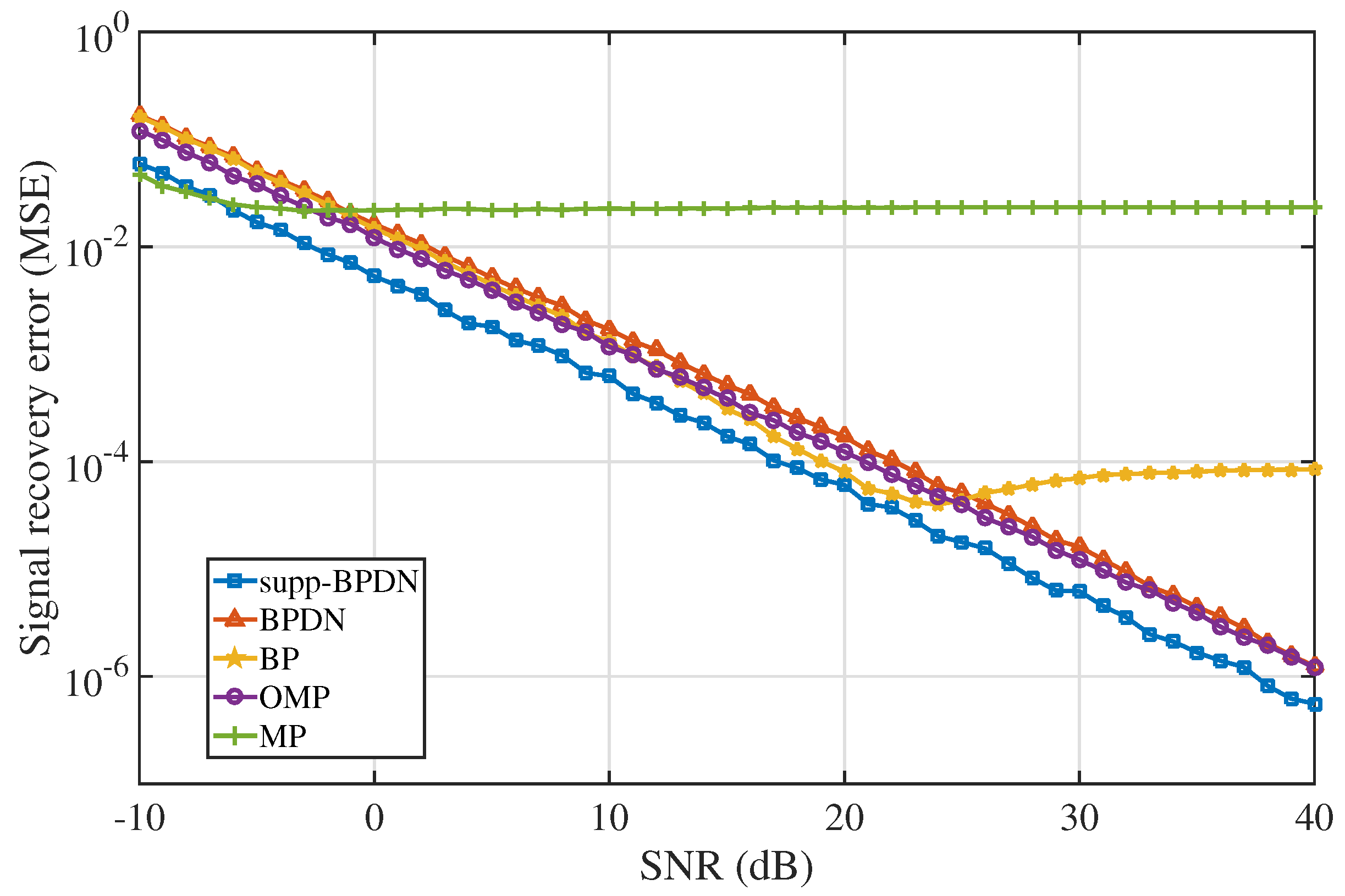
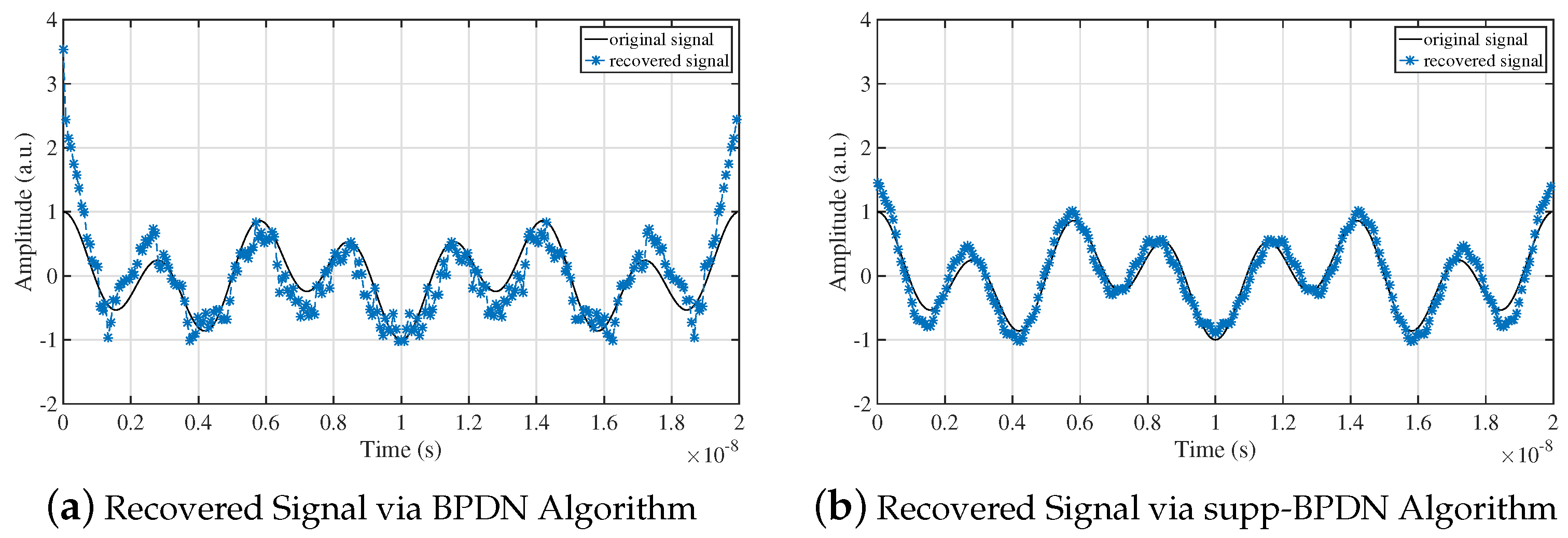
4. Numerical Simulations

In this section, a series of numerical simulations performed via CVX toolbox in Matlab are reported. In the simulations, N = 256 , (number of measurements) M = 64 , (original signal) s was the sum of three cosines of different frequencies, and the mathematical expression was
s t = a cos 2 π f 1 t + b cos 2 π f 2 t + c cos 2 π f 3 t ,
where f 1 = 50 MHz; f 2 = 150 MHz; f 3 = 350 MHz; and a, b, and c are constants, leading to sparsity k = 6 in frequency domain. Meanwhile, as the original signals are measured by PRBS in communication systems, we adopted a matrix in which 0 s and 1 s are randomly generated, and multiplied it with Fourier transform matrix Ψ as MM.
The first simulation compared the single recovery results of BPDN and supp-BPDN algorithms, as shown in the Figure 1. Noise was present in this situation, and we set signal-to-noise ratio (SNR) of CS system to 5 dB; the parameters used in reconstruction algorithm were λ = 0.05 2 log N , t = 3 k , and other parameters were the same as above settings. It can be seen that in Figure 1a, although frequencies of the original signal were recovered accurately, there was some wrong information recovered as well, which resulted in recovery errors. However, in Figure 1b, it is obvious that the recovered result is more “clear” outside the range of supp x than with the supp-BPDN algorithm.
The second simulation exhibits the signal recovery performances of BP, BPDN, MP, OMP, and supp-BPDN algorithms when the system signal-to-noise ratio (SNR) changed. Quality of reconstruction result was measured by mean square error (MSE):
MSE = 1 N i = 1 N s i s ^ i 2 ,
where s ^ is the reconstructed signal and s is the original signal.
In the simulation, SNR of the system increased from −10 to 40 dB and the step size was 1 dB. Under each variation, the algorithms were executed 100 times; we obtained recovery errors and averaged them. Results are shown in Figure 2; the performance of supp-BPDN was better than those of BPDN and BP algorithms in the entire SNR range. Curves of supp-BPDN and BPDN exhibit the same tendency in general; in the range of −5 to 25 dB, recovery errors of BP are less than those of BPDN, caused by the overly pessimistic characteristic of BPDN upon encountering noise mentioned in Section 2.
In the next simulation, reconstruction performances among supp-BPDN, BPDN, BP, and OMP algorithms were obtained for numbers of measurements M ranging from 50 to 150. Likewise, we set N = 256 , λ = 0.05 2 log N , iterations to 100, and SNR to 15 dB. The results are demonstrated in Figure 3. Similarly, supp-BPDN performed the best in the whole range. The curve of supp-BPDN shows a little decrease as M increases; there are small fluctuations during the variation. Additionally, a stable period with a little rise is shown in the curve of BPDN.
The last simulation aimed to exhibit signal recovery performances among supp-BPDN, BPDN, and OMP algorithms. Distinctively, in this simulation, we used a different noise model:
y noise = y + σ w ,
where w was the normalized Gaussian white noise. In this model, λ was no longer a constant, but a variable corresponding to the noise level σ , and the mapping relation was
λ σ = σ 2 log N .
Similarly, we set M = 64 , N = 256 , and circulation times to 3000. For every noise level, we repeated these algorithms 100 times. Recovery results are shown in Figure 4. When the noise level is from 0.01 to 0.1, curves of BPDN and OMP possess a steeper slope; recovery error is more steady in supp-BPDN.

5. CS System for Microwave Photonics

In this section, we present the design of a photonic-assisted CS system to verify the feasibility and superiority of the supp-BPDN algorithm in pratical situations.

5.1. System Setup

The layout of the proposed scheme is shown in Figure 5. Firstly, a continuous wave (CW) laser is used to generate continuous wave regarded as an optical carrier propagating in single mode fiber (SMF). Additionally, the light is modulated by the sparse-frequency radio frequency (RF) signal s t during the first MZM. After that, the optical signal carrying information enters the second MZM to be modulated another time. During this step, known PRBS patterns are encoded on the optical wave, yielding a multiplied signal whose RF signal is mixed with PRBS patterns to propagate into PD, transforming it into an electrical signal. Both MZMs are worked at the quadrature bias point. After PD and the amplifier, the signal is integrated during each period by the integrator. Finally, an ADC with a much lower sampling rate than the Nyquist frequency is applied to digitalize the measurements y , and recovery algorithms are used to reconstruct signals.
According to the mathematical model of CS theory, we can realize that there are two steps to establish a CS system, which are mixing and integrating. In the scheme shown in Figure 5, the original signal is mixed with MM via MZMs in the photonic link, and integration process is realized in an electrical circuit. It is noteworthy that if MM is an M × N matrix, it means M measurement times are needed using M groups of PRBS. It should be noted that the length of the signal during each measurement period must be the same as that of PRBS; otherwise, aliasing and measuring confusion will occur, which brings errors to the reconstruction results. There is no need to use the system every single measurement; we can get M number of measurements during one execution.

5.2. Results and Discussion

We set up a CS system shown in Figure 5 by OptiSystem and recovered a two-tone signal of 350 and 150 MHz by a 200-MHz ADC, and a two-tone signal of 1 GHz and 600 MHz with a 500-MHz ADC.
In the system, the output optical power of the first MZM is
P out 1 = 1 2 1 + s t ,
where s t is the normalized original signal, voltages of which range from −1 to 1 V. Additionally, after different PRBS modulate the optical wave, the output power of the second MZM is
P out 2 = 1 2 r t 1 + s t ,
in which r t is the PRBS. Meanwhile, modulated waveforms of MZMs are shown in Figure 6, demonstrating a single period of signals in time domain. Figure 6a shows the original signal, and Figure 6b exhibits the original signal encoded by PRBS being measured.
From Equation (50), after PD and the integrator, PRBS is integrated by a period as well. Therefore, data sampled by ADC are actually two integral values, which is
y ^ m = α T 1 2 r m t 1 + s t d t = α 2 T r m t s t d t + 1 2 T r m t d t ,
where y ^ m is the m th measurement in practical systems, and r m t is the m th group of PRBS. α is a constant coefficient of the CS system, which is different when parameters change.
Figure 7 shows signals recovered by BPDN and supp-BPDN algorithms. The time interval of a period was 20 ns, the length of a group of PRBS was 256, measurement times M = 64 , the system SNR was 15 dB, and the sampling rate of ADC was 200 MHz. We can figure out that signals recovered by supp-BPDN were the most coincident with the original signal.
In the next simulation, we changed the frequencies of signal to 1 GHz and 600 MHz, and the sampling rate of ADC was 500 MHz; recovery results are shown in Figure 8. Similarly, supp-BPDN demonstrated better performance at recovering signals.

6. Conclusions

A novel signal recovery algorithm named supp-BPDN is put forward in this paper based on the theoretical analysis of the signal support set. This algorithm executes the step of selecting the signal support set before the traditional recovery algorithm BPDN; in other words, it selects the position indexes corresponding to the top t values of the inner products and only retains the recovery information in said position indexes, which can effectively avoid errors from wrong information. In the proposed algorithm, it is not necessary to remove the contributions of local optimal values in measurements y during each iteration, which simplifies the procedure. By means of numerical simulations, we compared supp-BPDN and traditional algorithms, and supp-BPDN had the best performances. Moreover, based on the advantages of microwave photonic technologies, a photonic-enabled CS system was designed to verify the proposed algorithm. Additionally, a signal with a maximum frequency of 350 MHz can be recovered when digitalized at 200 MHz. Moreover, a signal with a peak of 1 GHz could be reconstructed when digitalized at 500 MHz, achieving a breakthrough in the Nyquist sampling rate. Similarly, signals recovered by supp-BPDN fit the original signals more closely.

Author Contributions

Conceptualization, W.L. and Z.W.; software, W.L.; validation, W.L., Z.W., G.L. and Y.J.; writing—original draft preparation, W.L.; writing—review and editing, Z.W.; supervision, Z.W. and Y.J. All authors have read and agreed to the published version of the manuscript.

Funding

This work was supported by the National Natural Science Foundation of China under grant 61835003.

Conflicts of Interest

The authors declare no conflict of interest.

Abbreviations

The following abbreviations are used in this manuscript:
CSCompressive sensing
DOADirection of arrival
CRCognitive radio
MMMeasurement matrix
PRBSPseudo random bit sequence
ADCAnalog-to-digital converter
RIPRestricted isometry property
PDPhotodiode
NPHNon-deterministic polynomial hard
BPBasis pursuit
BPDNBasis pursuit denoising
SNRSignal-to-noise ratio
MSEMean square error
RDRandom demodulator
SLMSpatial light modulator
MZMMach–Zehnder modulator
MPMatching pursuit
LPFLow-pass filter
RICRestricted isometry constant
CWContinuous wave
SMFSingle mode fiber
RFRadio frequency
BCSBayesian compressive sensing
OMPorthogonal matching pursuit

References

  1. Emmanuel, J.C.; Romberg, J.; Tao, T. Robust Uncertainty Principles: Exact Signal Reconstruction From Highly Incomplete Frequency Information. IEEE Trans. Inf. Theory 2006, 52, 489–509. [Google Scholar]
  2. David, L.D. Compressed Sensing. IEEE Trans. Inf. Theory 2006, 52, 1289–1306. [Google Scholar]
  3. Cohen, D.; Eldar, Y.C. Sub-Nyquist Radar Systems. IEEE Signal Process. Mag. 2018, 11, 35–58. [Google Scholar] [CrossRef] [Green Version]
  4. Marco, F. Duarte; Mark A. Davenport; Dharmpal Takhar. Single-Pixel Imaging via Compressive Sampling. IEEE Signal Process. Mag. 2008, 3, 83–91. [Google Scholar]
  5. Lustig, M.; Donoho, D.; Pauly, J.M. Sparse MRI: The Application of Compressed Sensing for Rapid MR Imaging. Magn. Reson. Med. 2007, 58, 1182–1195. [Google Scholar] [CrossRef] [PubMed]
  6. Lei, C.; Wu, Y.; Sankaranarayanan, A.C. GHz Optical Time-Stretch Microscopy by Compressive Sensing. IEEE Photon. J. 2017, 9. [Google Scholar] [CrossRef]
  7. Shen, Q.; Liu, W.; Cui, W.; Wu, S. Underdetermined DOA Estimation Under the Compressive Sensing Framework: A Review. IEEE Access 2017, 4, 8865–8878. [Google Scholar] [CrossRef]
  8. Bazerque, J.A.; Giannakis, G.B. Distributed Spectrum Sensing for Cognitive Radio Networks by Exploiting Sparsity. IEEE Trans. Signal Process. 2010, 58, 1847–1862. [Google Scholar] [CrossRef]
  9. Nyquist, H. Gertain Factors Affecting Telegraph Speed. Bell Syst. Tech. J. 1928, 124–130. [Google Scholar]
  10. Shannon, C.E. A Mathematical Theory of Communication. Bell Syst. Tech. J. 1948, 27, 379–423. [Google Scholar] [CrossRef] [Green Version]
  11. Tropp, J.A.; Laska, J.N.; Laska, J.N. Beyond Nyquist: Efcient Sampling of Sparse Bandlimited Signals. IEEE Trans. Inf. Theory 2009, 56, 520–544. [Google Scholar] [CrossRef] [Green Version]
  12. Mishali, M.; Eldar, Y.C. From Theory to Practice: Sub-Nyquist Sampling of Sparse Wideband Analog Signals. IEEE J.-STSP 2010, 4, 375–391. [Google Scholar] [CrossRef] [Green Version]
  13. Nichols, J.M.; Bucholtz, F. Beating Nyquist with light: A compressively sampled photonic link. Opt. Express 2011, 19, 7339–7348. [Google Scholar] [CrossRef]
  14. Chi, H.; Mei, Y.; Chen, Y. Microwave spectral analysis based on photonic compressive sampling with random demodulation. Opt. Lett. 2012, 37, 4636–4638. [Google Scholar] [CrossRef]
  15. Chen, Y.; Chi, H.; Jin, T. Sub-Nyquist Sampled Analog-to-Digital Conversion Based on Photonic Time Stretch and Compressive Sensing With Optical Random Mixing. J. Light. Technol. 2013, 31, 3395–3401. [Google Scholar] [CrossRef]
  16. Liang, Y.; Chen, M.; Chen, H. Photonic-assisted multi-channel compressive sampling based on effective time delay pattern. Opt. Express 2013, 21, 25700–25707. [Google Scholar] [CrossRef] [PubMed]
  17. Bosworth, B.T.; Foster, M.A. High-speed ultrawideband photonically enabled compressed sensing of sparse radio frequency signals. Opt. Lett. 2013, 38, 4892–4895. [Google Scholar] [CrossRef] [PubMed]
  18. Chi, H.; Chen, Y.; Mei, Y. Microwave spectrum sensing based on photonic time stretch and compressive sampling. Opt. Lett. 2013, 38, 136–138. [Google Scholar] [CrossRef] [PubMed]
  19. Chen, Y.; Yu, X.; Chi, H. Compressive sensing in a photonic link with optical integration. Opt. Lett. 2014, 39, 2222–2224. [Google Scholar] [CrossRef] [Green Version]
  20. Guo, Q.; Liang, Y.; Chen, M. Compressive spectrum sensing of radar pulses based on photonic techniques. Opt. Express 2015, 23, 4517–4522. [Google Scholar] [CrossRef]
  21. Bosworth, B.T.; Stroud, J.R.; Tran, D.N. Ultrawideband compressed sensing of arbitrary multi-tone sparse radio frequencies using spectrally encoded ultrafast laser pulses. Opt. Lett. 2015, 40, 3045–3048. [Google Scholar] [CrossRef]
  22. Chi, H.; Zhu, Z. Analytical Model for Photonic Compressive Sensing With Pulse Stretch and Compression. IEEE Photon. J. 2019, 11, 5500410. [Google Scholar] [CrossRef]
  23. Zhu, Z.; Chi, H.; Jin, T. Photonics-enabled compressive sensing with spectral encoding using an incoherent broadband source. Opt. Lett. 2018, 43, 330–333. [Google Scholar] [CrossRef] [PubMed]
  24. Valley, G.C.; Sefler, G.A.; Shaw, T.J. Compressive sensing of sparse radio frequency signals using optical mixing. Opt. Lett. 2012, 37, 4675–4677. [Google Scholar] [CrossRef] [PubMed]
  25. Chen, S.S.; Donoho, D.L.; Saunders, M.A. Atomic Decomposition by Basis Pursuit. SIAM Rev. 2001, 43, 129–159. [Google Scholar] [CrossRef] [Green Version]
  26. Hale, E.T.; Yin, W.; Zhang, Y. Fixed-Point Continuation for 1-Minimization: Methodology and Convergence. Siam J. Optim. 2008, 19, 1107–1130. [Google Scholar] [CrossRef]
  27. Mallat, S.G.; Zhang, Z. Matching pursuits with time-frequency dictionaries. IEEE Trans. Signal Process. 1993, 41, 3397–3415. [Google Scholar] [CrossRef] [Green Version]
  28. Tropp, J.A.; Gilbert, A.C. Signal Recovery From Random Measurements Via Orthogonal Matching Pursuit. IEEE Trans. Inf. Theory 2007, 53, 4655–4666. [Google Scholar] [CrossRef] [Green Version]
  29. Needell, D.; Tropp, J.A. CoSaMP: Iterative signal recovery from incomplete and inaccurate samples. Appl. Comput. Harmon. Anal. 2008, 26, 301–321. [Google Scholar] [CrossRef] [Green Version]
  30. Lu, D.; Sun, G.; Li, Z.; Wang, S. Improved CoSaMP Reconstruction Algorithm Based on Residual Update. J. Comput. Commun. 2019, 7, 6–14. [Google Scholar] [CrossRef] [Green Version]
  31. Dai, L.; Wang, Z.; Yang, Z. Compressive Sensing Based Time Domain Synchronous OFDM Transmission for Vehicular Communications. IEEE J. Sel. Areas Commun. 2013, 31, 460–469. [Google Scholar]
  32. Zhang, W.; Li, H.; Kong, W.; Fan, Y.; Cheng, W. Structured Compressive Sensing Based Block-Sparse Channel Estimation for MIMO-OFDM Systems. Wireless Pers. Commun. 2019, 108, 2279–2309. [Google Scholar] [CrossRef]
  33. Ji, S.; Xue, Y.; Carin, L. Bayesian Compressive Sensing. IEEE Trans. Signal Process. 2008, 56, 2346–2356. [Google Scholar] [CrossRef]
  34. Wipf, D.P.; Rao, B.D. An Empirical Bayesian Strategy for Solving the Simultaneous Sparse Approximation Problem. IEEE Trans. Signal Process. 2007, 55, 3704–3716. [Google Scholar] [CrossRef]
  35. Oikonomou, V.P.; Nikolopoulos, S.; Kompatsiaris, I. A Novel Compressive Sensing Scheme under the Variational Bayesian Framework. In Proceedings of the European Signal Processing Conference, 27th European Signal Processing Conference (EUSIPCO), A Coruna, Spain, 2–6 September 2019. [Google Scholar]
  36. Candès, E.J. The restricted isometry property and its implications for compressed sensing. CR Math. 2008, 346, 589–592. [Google Scholar] [CrossRef]
  37. Eldar, Y.C.; Kutyniok, G. Compressed Sensing: Theory and Applications, 3rd ed.; Cambridge University Press: Cambridge, UK, 2013; pp. 25–26, 349–351. [Google Scholar]
  38. Baraniuk, R.; Davenport, M.; DeVore, R.; Wakin, M. A Simple Proof of the Restricted Isometry Property for Random Matrices. Constr. Approx 2008, 28, 253–263. [Google Scholar] [CrossRef] [Green Version]
  39. Cormen, T.H.; Leiserson, C.E.; Rivest, R.L.; Stein, C. Introduction to Algorithms, 3rd ed.; MIT Press: Cambridge, MA, USA, 2009; pp. 616–623. [Google Scholar]
  40. Donoho, D.L. De-noising by soft-thresholding. IEEE Trans. Inf. Theory 1995, 41, 613–627. [Google Scholar] [CrossRef] [Green Version]
Figure 1. Spectra of original and reconstructed signals recovered by supp-BPDN and BPDN. (a) Reconstruction result of frequencies by BPDN. (b) Reconstruction result of frequencies by the proposed algorithm.
Electronics 10 01544 g001
Figure 2. Signal reconstruction errors with respect to SNR among supp-BPDN, BPDN, BP, OMP, and MP algorithms using the logarithmic (base 10) scale for the y-axis.
Electronics 10 01544 g002
Figure 3. Signal reconstruction error with respect to different numbers of measurements M among supp-BPDN, BPDN, BP, and OMP algorithms.
Electronics 10 01544 g003
Figure 4. Signal recovery errors with respect to noise level among supp-BPDN, BPDN, and OMP algorithms.
Electronics 10 01544 g004
Figure 5. Scheme of the proposed CS system. CW laser: continuous wave laser; MZM: Mach–Zehnder modulator; PD: photodiode; RFA: amplifier; ∫: integrator; ADC: analog-to-digital converter; dashed line: optical link (single mode fiber); solid line: electrical circuit.
Electronics 10 01544 g005
Figure 6. Waveforms of modulated signals. (a) One period of original signal. (b) One period of mixed signal.
Electronics 10 01544 g006
Figure 7. Comparison of original and reconstructed signals under BPDN and supp-BPDN algorithms. Frequencies of signal were 350 MHz and 150 MHz; sampling rate was 200 MHz. (a) Signal recovered by BPDN. (b) Signal recovered by supp-BPDN.
Electronics 10 01544 g007
Figure 8. Comparison of original and reconstructed signals using BPDN and supp-BPDN algorithms. Frequencies of signal were 1 GHz and 600 MHz; sampling rate was 500 MHz. (a) Signal recovered by BPDN. (b) Signal recovered by supp-BPDN.
Electronics 10 01544 g008
Publisher’s Note: MDPI stays neutral with regard to jurisdictional claims in published maps and institutional affiliations.

