
Models of Air Pollution Propagation in the Selected Region of Katowice


Abstract
1. Introduction
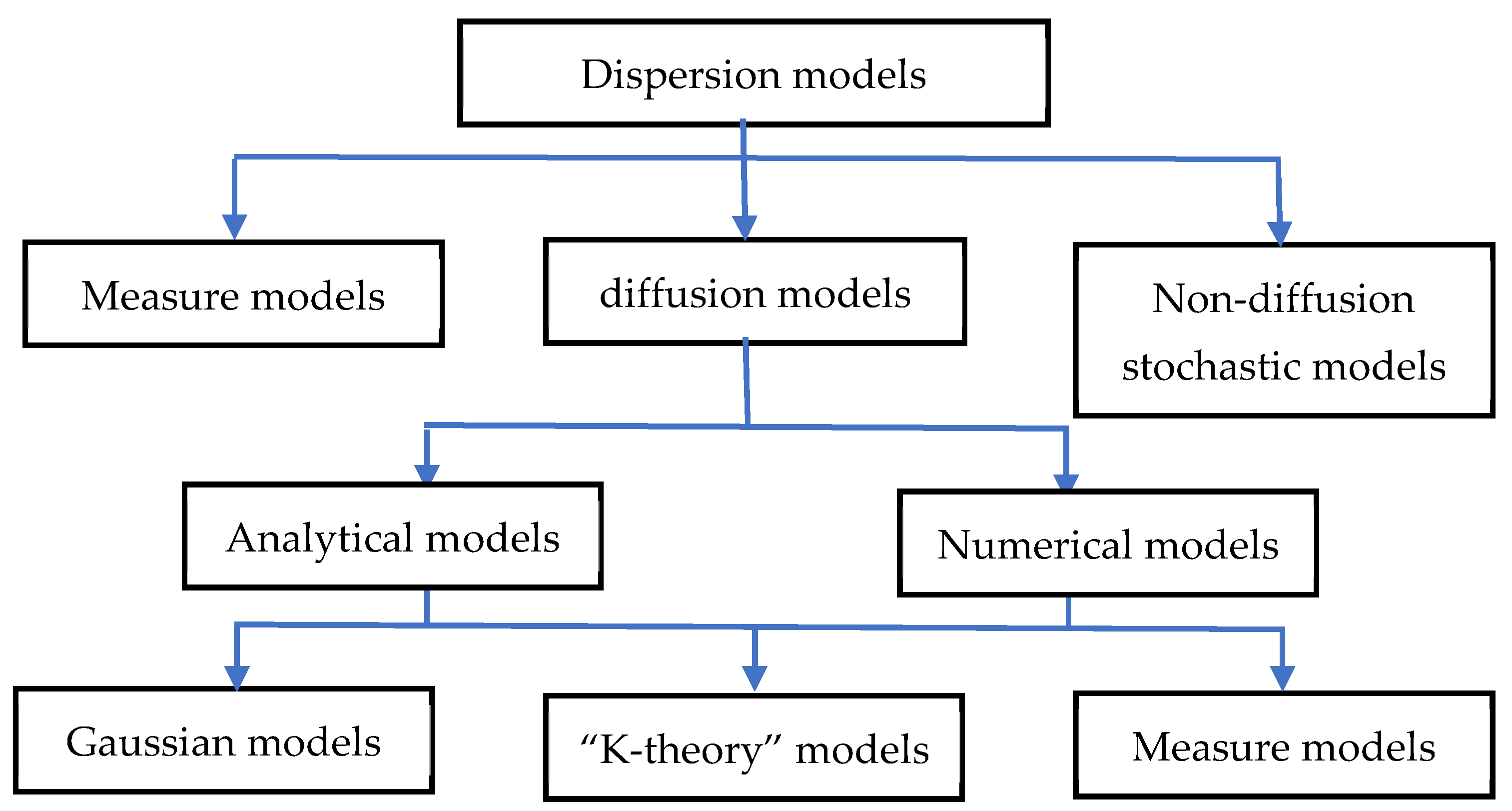
2. Models of Air Pollution Propagation
3. Correlation Analysis and Data Analysis
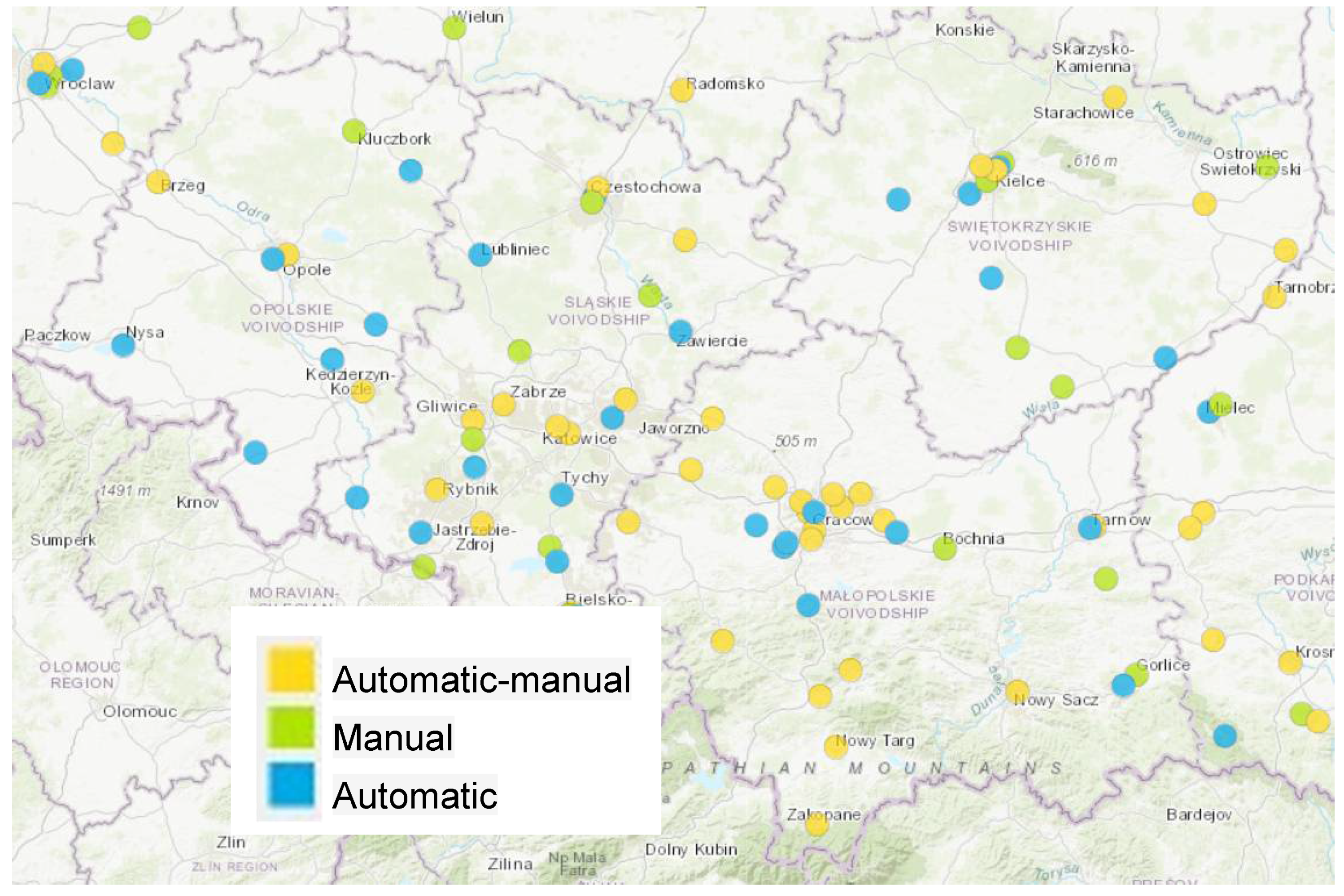
3.1. Information about Data
3.2. Correlation
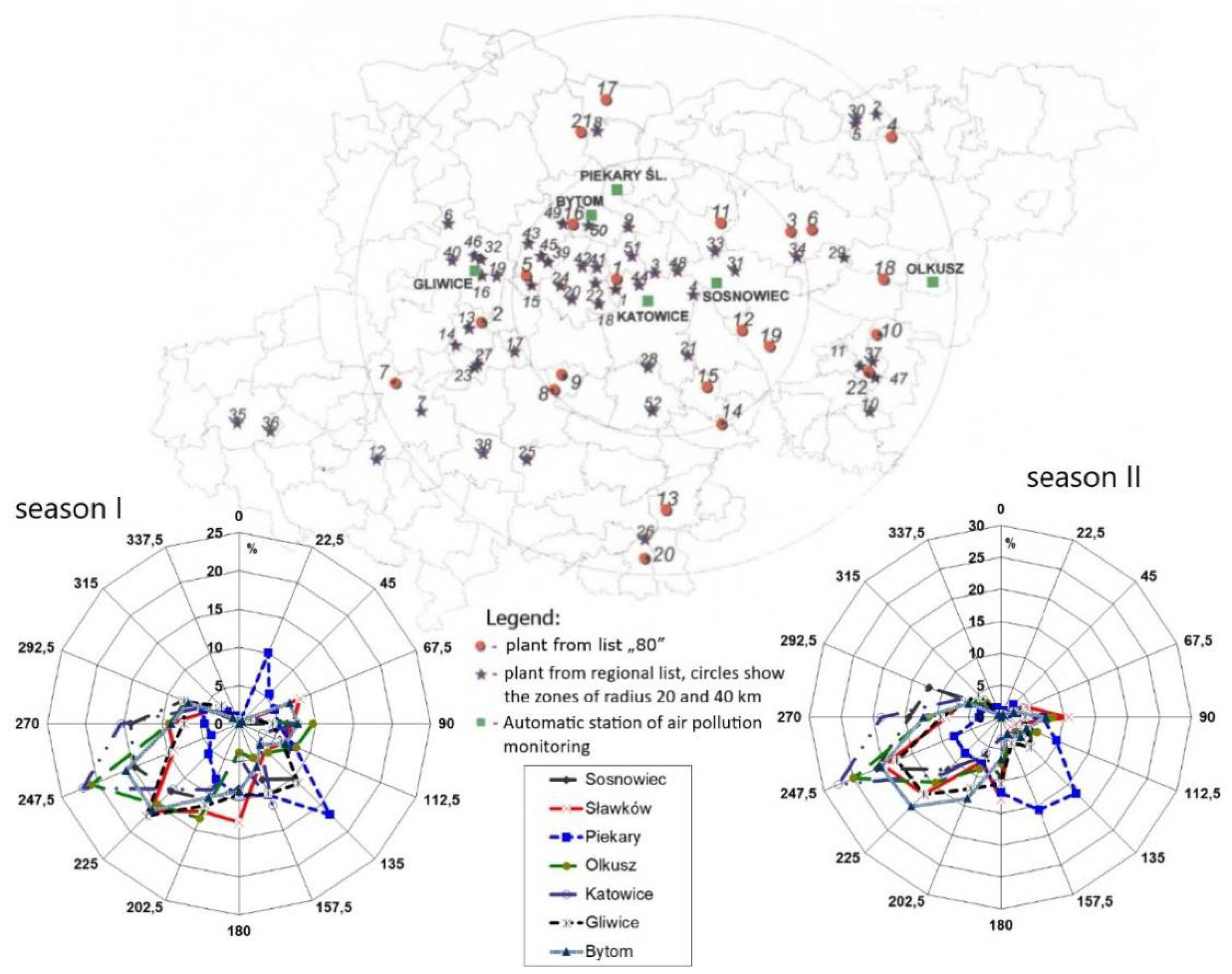
3.3. Wind Roses
- days in which air inflow at all stations came from quadrant (180°, 270°);
- days in which air inflow at certain station came from quadrant (180°, 270°);
- remaining days separately for heating seasons 1996–1997 and 1997–1998.
3.4. Summary Statistics
4. Modelling Results and Discussion
- Regression model for SO2 concentrations in the heating season 2013–2014, Katowice, Kossuth Street.
- Regression model for SO2 concentrations in the heating season 2014–2015, Katowice, Kossuth street.
- Regression model for SO2 concentrations in the heating season 2015–2016, Katowice, Kossuth street.
- Regression model for SO2 concentrations in three heating seasons 2013–2016 total, Katowice, Kossuth Street.
- Regression model for PM10 concentration for heating season 2013–2014, Katowice, Kossuth Street.
- Regression model for PM10 concentration for heating season 2014–2015, Katowice, Kossuth Street.
- Regression model for PM10 concentration for heating season 2015–2016, Katowice, Kossuth Street.
- Regression model for PM10 concentrations for all three heating seasons 2013–2016, Katowice, Kossuth Street.
5. Conclusions
- -
- There is a high correlation between SO2 and dust concentrations at moment t and previous concentrations. The correlation coefficients between individual pollutants measured at the same time are at a satisfactory level.
- -
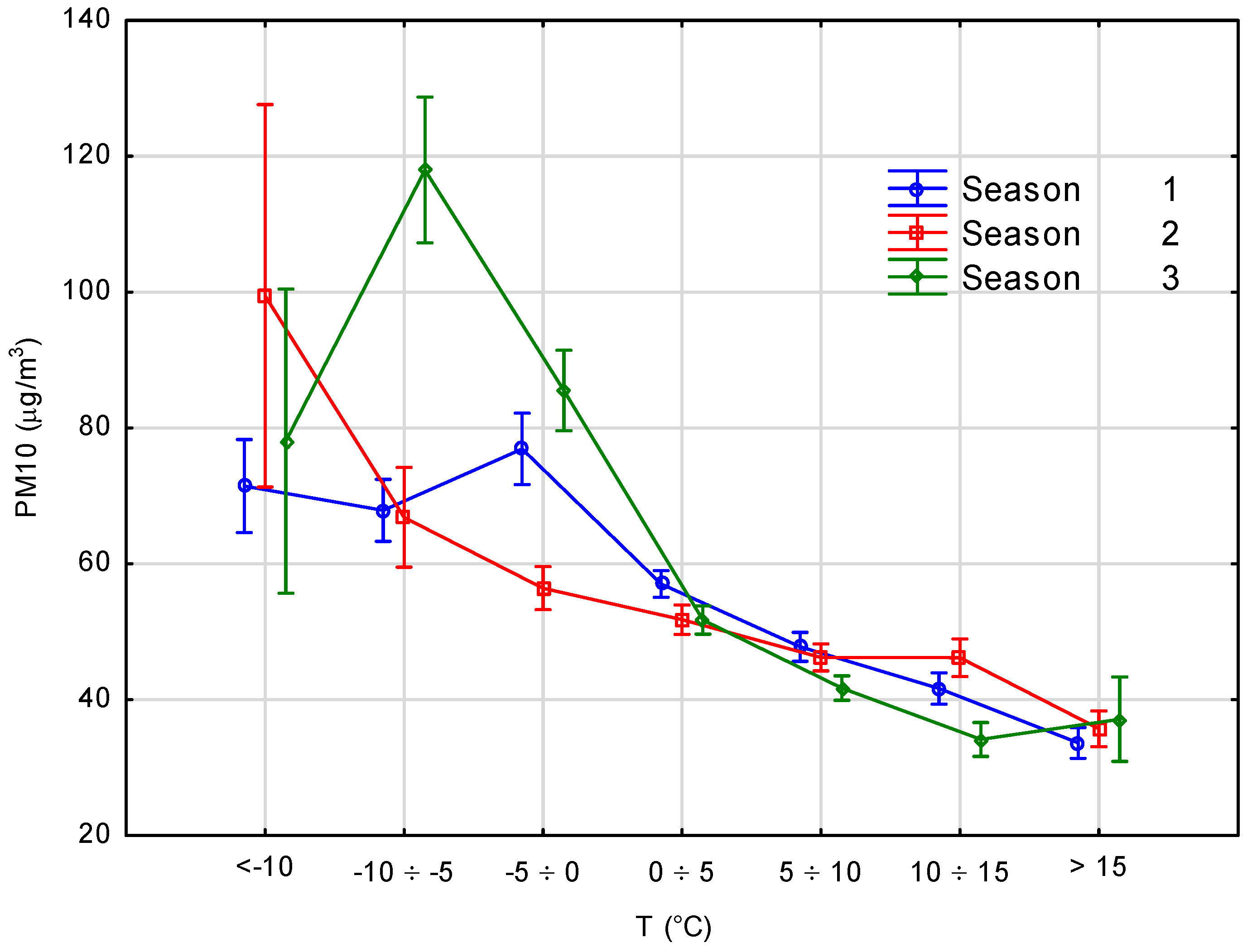
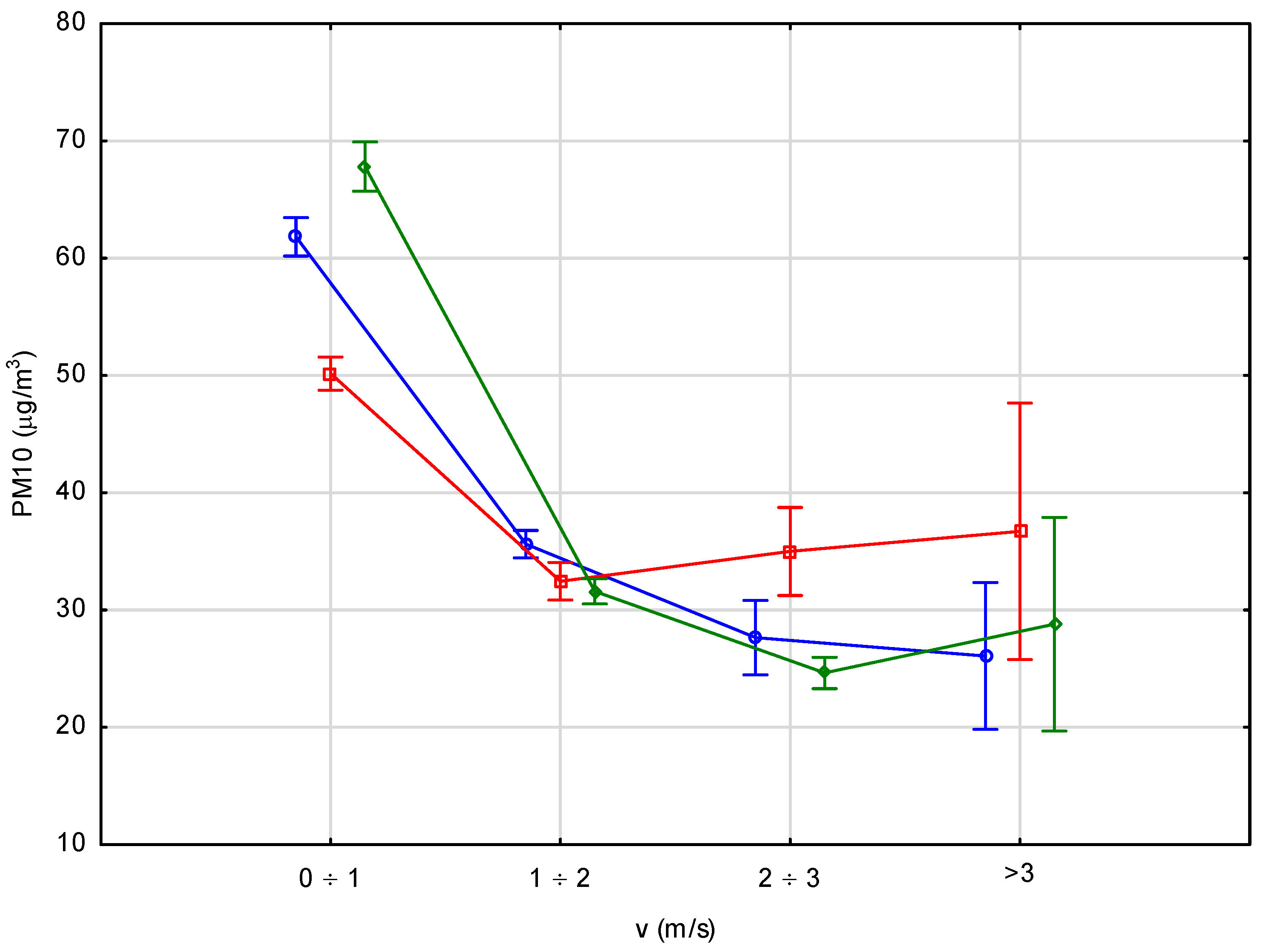
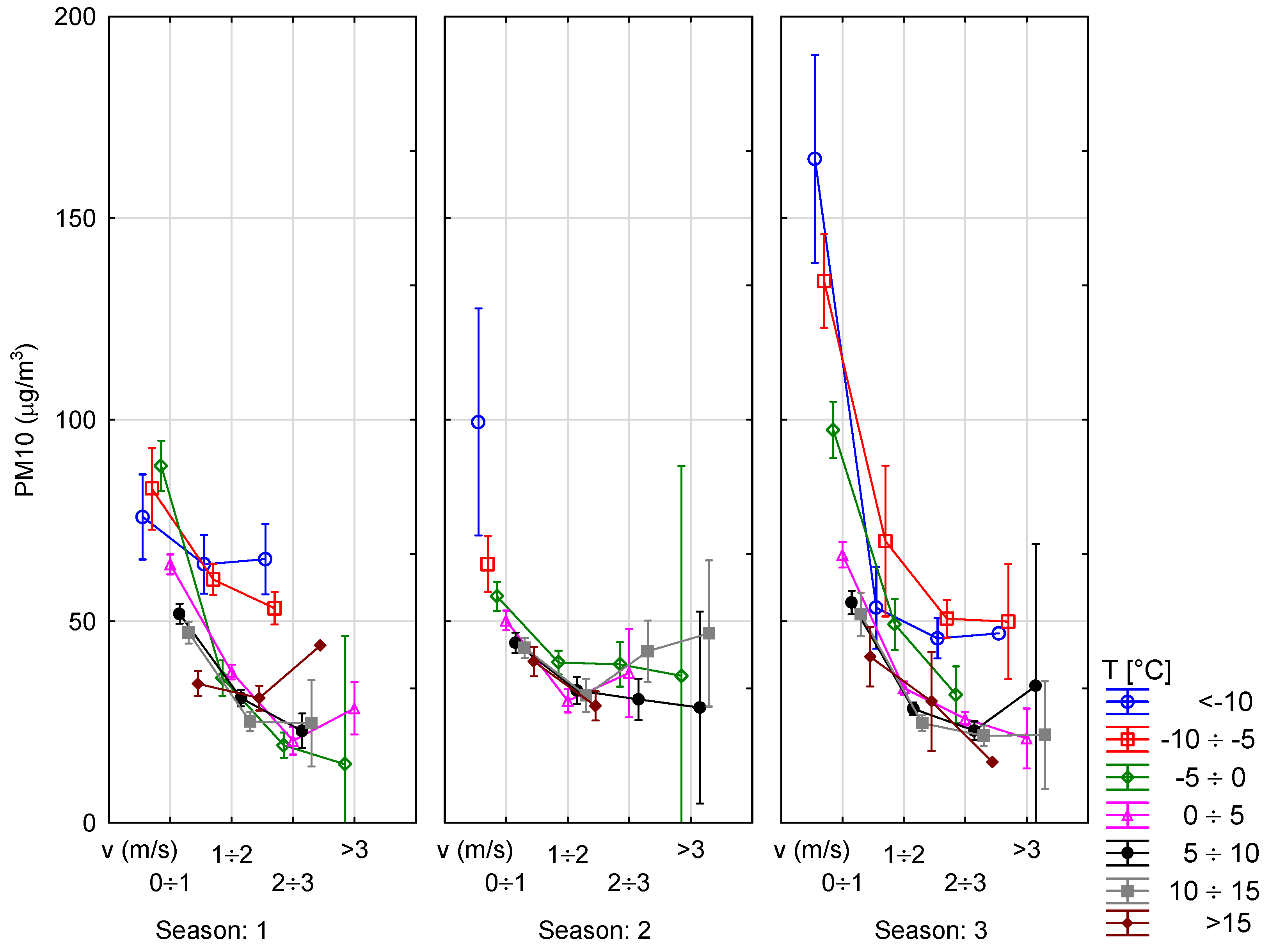
- The proposed form of the model can generate good starting material when attempting to create a stochastic model that, depending on the direction of research, might provide better results for predicting concentrations of the studied type of air pollution. The analyses confirmed the parabolic character of the relationship between SO2 and PM10 concentrations and the meteorological parameters of wind speed and temperature. This was especially visible for low temperature values. Forr SO2, the mean concentration for low temperatures was around 30–40 µg/m3 and for higher values around 15. In case of PM10 the same relations were 70–120 µg/m3 and for positive values, 30–50 µg/m3.
- -
- The results obtained from individual heating seasons were similar to the results obtained from analyzing the years 2013–2016, as a whole.
- -
- The application of the above-mentioned statistical methods describing the measurement data obtained from the station allows for the analysis of their quantitative and qualitative dependencies, which is not always possible when using only numerical models or estimation methods (e.g., neural networks). The obtained errors were quite comparable for all seasons. In case of SO2 it was equal to about 5 µg/m3 and in case of PM10 around 15 µg/m3.
- -
- The proposed model can be treated as a unified form. Even if the model from a previous year is used for a new one, the fit is quite good. The very important parameter in the model is the accumulation of s pollutant from a previous time. That means that the model coefficients are quite stable for s certain area. They may change if area’s urbanization or location of industrial plants changes.
- -
- The observation of the model coefficient values and variations, as well as the influence of meteorological conditions (wind speed and temperature) allows an eventual evaluation of the effects of activities to change heating systems in buildings as described at the beginning of the paper.
Author Contributions
Funding
Institutional Review Board Statement
Informed Consent Statement
Data Availability Statement
Acknowledgments
Conflicts of Interest
References
- Kleczkowski, P. Smog w Polsce; Wydawnictwo Naukowe PWN: Warszawa, Poland, 2019. [Google Scholar]
- Moussiopoulos, N. (Ed.) Air Quality in Cities; SATURN—EUROTRAC 2 Subproject Report; Springer: Berlin/Heidelberg, Germany, 2003. [Google Scholar]
- Polski Alarm Smogowy. Available online: polskialarmsmogowy.pl (accessed on 30 November 2020).
- Kobus, D.; Merenda, B.; Sówka, I.; Chlebowska-Styś, A.; Wroniszewska, A. Ambient air quality as a condition of effective healthcare therapy on the example of selected Polish health resorts. Atmosphere 2020, 11, 882. [Google Scholar] [CrossRef]
- Wielgosiński, G.; Czerwińska, J. Smog Episodes in Poland. Atmosphere 2020, 11, 277. [Google Scholar] [CrossRef]
- Foszcz, D.; Niedoba, T.; Saramak, D.; Gawenda, T. The Methodology of the SO2 Concentration Forecasting in the Cities for the Preventive Purposes in the Example of the City of Kraków. In Proceedings of the 3rd International Conference of PhD Students, Engineering Sciences, Miskolc, Hungary, 13–19 August 2001; Volume 2, pp. 569–576. [Google Scholar]
- Foszcz, D.; Niedoba, T.; Siewior, J. The Methods of Forecasting of SO2 and Suspended Dust Concentrations for Warning Purposes in the Example of Selected Polluted Regions in Poland. In Ecosystems and Sustainable Development; Tiezzi, E., Brebbia, C.A., Jorgensen, S., Almorza Gomar, D., Eds.; WIT Press: Southampton/Boston, UK, 2005; pp. 477–491. [Google Scholar]
- Kunysz, J.; Foszcz, D.; Gawenda, T.; Tumidajski, T. Modele adaptacyjne jako metoda prognozowania średniodobowych stężeń SO2. Ochr. Powietrza Probl. Odpadów 2001, 35, 138–143. [Google Scholar]
- Siewior, J.; Tumidajski, T.; Foszcz, D.; Niedoba, T. Prognozowanie stężeń zanieczyszczeń powietrza w GOP-ie modelami statystycznymi. Rocz. Ochr. Sr. 2011, 13, 1261–1274. [Google Scholar]
- Tumidajski, T.; Siewior, J.; Foszcz, D.; Niedoba, T. Ocena wpływu stężeń zanieczyszczeń powietrza w GOP-ie na jakość powietrza w rejonie Opola i Kędzierzyna-Koźla. Rocz. Ochr. Sr. 2014, 16, 519–533. [Google Scholar]
- Bringfelt, B. Important factors for the sulphur dioxide concentration in central Stockholm. Atmos. Environ. 1971, 5, 949–972. [Google Scholar] [CrossRef]
- Bolzern, P.; Fronza, G.; Runze, E.; Uberhuber, C. Statistical analysis of winter sulphur dioxide concentration data in Vienna. Atmos. Environ. 1982, 16, 1899–1906. [Google Scholar] [CrossRef]
- Hysenaj, M. Dispersion model prospective of air pollution in Tirana. Geogr. Tech. 2019, 14, 10–19. [Google Scholar] [CrossRef]
- Markiewicz, M.T. Methods of determining meteorological data used in air pollution dispersion models. Environ. Prot. Eng. 2007, 33, 75–86. [Google Scholar]
- Markiewicz, M.T. Podstawy Modelowania Rozprzestrzeniania Się Zanieczyszczeń w Powietrzu Atmosferycznym; Oficyna Wydawnicza Politechniki Warszawskiej: Warsaw, Poland, 2004. [Google Scholar]
- Markiewicz, M.T. Methods of the wet deposition description in air pollution dispersion models. Environ. Prot. Eng. 2007, 33, 113–120. [Google Scholar]
- Carmichael, C.R.; Peters, L.K.; Saylor, R.D. The STEM II regional scale acid deposition model: Physical concept and formulation. Part I. Atmos. Environ. 1991, 25, 2077–2090. [Google Scholar] [CrossRef]
- Chang, J.S.; Brost, R.A.; Isaksen, P.S.A.; Madronich, S.; Middleton, P.; Stockwell, W.R.; Walcek, C.J. A three-dimensional Eulerian acid desposition model. Physical concepts and formulation. J. Geophys. Res. 1987, 92, 14681–14700. [Google Scholar] [CrossRef]
- Venkatram, A.; Karamandani, P.K. Testing a comprehensive acid deposition model. Atmos. Environ. 1989, 22, 737–747. [Google Scholar] [CrossRef]
- Hamer, P.D.; Walker, S.-E.; Sousa-Santos, C.; Vogt, M.; Vo-Thanh, D.; Lopez-Aparicio, S.; Schneider, P.; Ramacher, M.O.P.; Karl, M. The urban dispersion model EPISODE v. 10.0—Part I: An Eulerian and sub-grid scale air quality model and its application in Nordic winter conditions. Geosci. Model. Dev. 2020, 13, 4323–4353. [Google Scholar] [CrossRef]
- Cirtina, D.; Pecingina, J.; Cirtina, L. Study on Mathematical Modeling of the Dispersion Sulfur Dioxide by Burning Fossil Fuels. In Proceedings of the International Multidisciplinary Scientific GeoConference and EXPO SGEM, Albena, Bulgaria, 17–26 June 2014; pp. 523–531. [Google Scholar]
- Morawska-Horawska, M. Stochastyczne modele prognozy średniego dobowego stężenia SO2 dla Krakowa. Wiadomości IMGW 1988, 9, 3. [Google Scholar]
- Ilić, I.; Vuković, M.; Štrbac, N.; Urošević, S. Applying GIS to control transportation air pollutants. Pol. J. Environ. Stud. 2014, 23, 1849–1860. [Google Scholar]
- Vlaknenski, T.; Stoychev, P.; Chuturkova, R. Dispersion modeling of atmospheric emissions of particulate matter (PM10) and evaluation of the contribution of different sources of air pollution in the town of Svishtov, Bulgaria. J. Sci. Appl. Res. 2014, 5, 202–212. [Google Scholar]
- Zahron, E.M.M. A novel approach to improve the air quality predictions of air pollution dispersion modelling systems. Int. J. Environ. Res. 2013, 7, 205–218. [Google Scholar]
- El-Harbawi, M. Air quality model ling, simulation and computational methods: A review. Environ. Rev. 2013, 21, 149–179. [Google Scholar] [CrossRef]
- Juda-Rezler, K. Oddziaływanie Zanieczyszczeń Powietrza na Środowisko; Wyd. OWPW: Warsaw, Poland, 2006. [Google Scholar]
- Holnicki-Szulc, P. Modele Propagacji Zanieczyszczeń Atmosferycznych w Zastosowaniu do Kontroli i Sterowania Jakością Środowiska; Akademicka Oficyna Wydawnicza EXIT: Warsaw, Poland, 2006. [Google Scholar]
- Khoo, H.H.; Spedding, T.A.; Houston, D.; Taplin, D. Application of modeling and simulation tools in costs and pollution monitoring. Environmentalist 2001, 21, 161–168. [Google Scholar] [CrossRef]
- Gorai, A.K.; Upadhyay, A.K.; Goyal, P. Design of fuzzy synthetic evaluation model for air quality assessment. Environ. Syst. Decis. 2014, 34, 456–469. [Google Scholar] [CrossRef]
- Billiaiev, M.M.; Slavinska, O.S.; Kyrychenko, R.V. Numerical simulation of pollution dispersion in urban street. Ekol. Transporti 2017, 70, 23–28. [Google Scholar] [CrossRef]
- Jury, M.R.; Wilczak, J.M. Mesoscale numerical models: Cost-effective input to dispersion prediction schemes. Clean Air 1992, 8, 12–14. [Google Scholar] [CrossRef]
- Preto, W.H.; Cremasco, M.A. Application of probability density functions in modelling annual data of atmospheric NOx temporal concentration. Chem. Eng. Trans. 2017, 57, 487–492. [Google Scholar]
- Hammond, J.K.; Chen, R.; Mallet, V. Meta-modeling of a simulation chain for urban air quality. Adv. Mod. Simul. Eng. Sci. 2020, 7, 1–22. [Google Scholar]
- Kim, Y.; Wu, Y.; Seigneur, C.; Roustan, Y. Multi-scale modeling of urban air pollution: Development and application of a Street-in-Grid model (v1.0) by coupling MUNICH (v1.0) and Polair3D (v1.8.1). Geosci. Model Dev. 2018, 11, 611–629. [Google Scholar] [CrossRef]
- Chen, H.; Xue, B. Research on the factors affecting regional smog in China—Based on spatial panel model. Mod. Econ. 2019, 10, 1292–1309. [Google Scholar] [CrossRef][Green Version]
- Deng, L.; Yu, M.; Zhang, Z. Statistical learning of the worst regional smog extremes with dynamic conditional modeling. Atmosphere 2020, 11, 665. [Google Scholar] [CrossRef]
- Hu, D.; Jiang, J. A study of smog issues and PM2.5 pollutant control strategies in China. J. Environ. Prot. 2013, 4, 746–752. [Google Scholar] [CrossRef][Green Version]
- Yu, X.; Shen, M.; Shen, W.; Zhang, X. Effects of land urbanization on smog pollution in China: Estimation of spatial autoregressive panel data models. Land 2020, 9, 337. [Google Scholar] [CrossRef]
- Zwoździak, J. Prognozy i Analizy Stężeń Zanieczyszczeń w Powietrzu w Regionie Czarnego Trójkąta; Oficyna Wydawnicza Politechniki Wrocławskiej: Wrocław, Poland, 1998. [Google Scholar]
- Finzi, G.; Tebaldi, G. A mathematical model for air pollution forecast and alarm in an urban area. Atmos. Environ. 1982, 16, 2055–2090. [Google Scholar] [CrossRef]
- Rani, N.L.A.; Azid, A.; Khalit, S.I.; Juahi, H.; Samsudin, M.S. Air pollution index trend analysis in Malaysia, 2010–2015. Pol. J. Environ. Stud. 2018, 27, 801–807. [Google Scholar] [CrossRef]
- Hamid, A.; Atique, S.A.; Huma, Z.; Uddin, S.G.M.; Asghar, S. Ambient air quality & noise level monitoring of different areas of Lahore (Pakistan) and its health impacts. Pol. J. Environ. Stud. 2019, 28, 623–629. [Google Scholar]
- Huete-Morales, M.D.; Quesada-Rubio, J.-M.; Navarette Álvarez, E.; Rosales-Moreno, M.J.; Del-Moral-Ávila, M.J. Air quality analysis in the European union. Pol. J. Environ. Stud. 2017, 26, 1113–1119. [Google Scholar] [CrossRef]
- Saramak, A. Comparative analysis of indoor and outdoor concentration of PM10 particulate matter on example of Cracow City center. Int. J. Environ. Sci. Techol. 2019, 16, 6609–6616. [Google Scholar] [CrossRef]
- Spychała, M.; Domagajska, J.; Ćwieląg-Drabek, M.; Marchwińska-Wyrwał, E. Correlation between length of life and exposure to air pollution. Pol. J. Environ. Stud. 2020, 29, 1361–1368. [Google Scholar] [CrossRef]
- Baklanov, A.; Zhang, Y. Advances in air quality modeling and forecasting. Glob. Transit. 2020, 2, 261–270. [Google Scholar] [CrossRef]
- Nichol, J.E.; Bilal, M.; Qiu, Z. Air pollution scenario over China during COVID-19. Remote Sens. 2020, 12, 2100. [Google Scholar] [CrossRef]
- Dziennik Ustaw. J. Laws 2019, pos. 1355, as amended.
- Inspekcja Ochrony Środowiska. Available online: http://powietrze.gios.gov.pl/pjp/maps/measuringstation (accessed on 20 January 2021).
- Jarzębski, L. Raport o Stanie Środowiska w Województwie Katowickim w Latach 1995–1996; Biblioteka Monitoringu Środowiska: Katowice, Poland, 1997. [Google Scholar]
- Tumidajski, T.; Foszcz, D.; Gawenda, T. Wybrane aspekty zmian zanieczyszczeń powietrza miast Górnośląskiego Okręgu Przemysłowego. Zesz. Nauk. Wydziału Budownictwa Ŝynierii Sr. 2001, 20, 573–580. [Google Scholar]


| Model Group (Basic Classes) | Air Pollution Dispersion Models |
|---|---|
| Eulerian models | Box models |
| Analytical models | |
| Numerical, first-order closure models | |
| Numerical, higher-order closure models | |
| Large-scale eddy simulation models | |
| Lagrangian models | Box models |
| Particle models | |
| Gaussian models | Traditional plume models |
| New generation models | |
| Segmented plume or puff models |
| Meteorological Methods | Air Pollution Dispersion Models |
|---|---|
| Traditional methods | Traditional Gaussian plume models |
| Segmented Gaussian plume of Gaussian puff | |
| Eulerian box models | |
| Eulerian analytical models | |
| Meteorological pre-processors | New-generation Gaussian plume models |
| Eulerian numerical models with the 1st order closure | |
| Eulerian box models | |
| Lagrangian box models | |
| Segmented Gaussian plume or puff models | |
| Meteorological prognostic models | Eulerian numerical models with the 1st and higher order closure |
| Eulerian large-scale eddy simulation models | |
| Lagrangian particle models |
| Variable | Average | Standard Deviation | P (hPa) | Wind Direction (Degree) | V (m/s) | T (°C) | Humidity (%) | SO2 | PM10 | PM2.5 | SO2-1 | PM10-1 | PM2.5-1 | (v-v0)2 | (T-T0)2 |
|---|---|---|---|---|---|---|---|---|---|---|---|---|---|---|---|
| P (hPa) | 983.22 | 9.40 | 1.00 | −0.03 | −0.03 | −0.08 | −0.02 | 0.01 | 0.12 | 0.12 | 0.00 | 0.12 | 0.11 | 0.02 | 0.08 |
| Wind_direction (degree) | 178.35 | 90.19 | −0.03 | 1.00 | 0.13 | 0.17 | −0.01 | −0.17 | −0.23 | −0.23 | −0.16 | −0.22 | −0.22 | −0.14 | −0.20 |
| v (m/s) | 0.88 | 0.65 | −0.03 | 0.13 | 1.00 | 0.15 | −0.22 | −0.16 | −0.35 | −0.36 | −0.15 | −0.32 | −0.33 | −0.99 | −0.15 |
| T (°C) | 4.60 | 5.46 | −0.08 | 0.17 | 0.15 | 1.00 | −0.34 | −0.33 | −0.27 | −0.34 | −0.31 | −0.26 | −0.33 | −0.16 | −0.97 |
| Humidity (%) | 78.73 | 14.84 | −0.02 | −0.01 | −0.22 | −0.34 | 1.00 | −0.02 | 0.10 | 0.17 | −0.05 | 0.10 | 0.16 | 0.21 | 0.28 |
| SO2 | 15.85 | 11.44 | 0.01 | −0.17 | −0.16 | −0.33 | −0.02 | 1.00 | 0.59 | 0.61 | 0.89 | 0.58 | 0.61 | 0.16 | 0.35 |
| PM10 | 50.44 | 41.10 | 0.12 | −0.23 | −0.35 | −0.27 | 0.10 | 0.59 | 1.00 | 0.98 | 0.54 | 0.94 | 0.92 | 0.36 | 0.27 |
| PM2.5 | 40.56 | 35.51 | 0.12 | −0.23 | −0.36 | −0.34 | 0.17 | 0.61 | 0.98 | 1.00 | 0.57 | 0.93 | 0.94 | 0.37 | 0.34 |
| SO2-1 | 15.86 | 11.45 | 0.00 | −0.16 | −0.15 | −0.31 | −0.05 | 0.89 | 0.54 | 0.57 | 1.00 | 0.59 | 0.61 | 0.14 | 0.33 |
| PM10-1 | 50.47 | 41.14 | 0.12 | −0.22 | −0.32 | −0.26 | 0.10 | 0.58 | 0.94 | 0.93 | 0.59 | 1.00 | 0.98 | 0.33 | 0.27 |
| PM2.5-1 | 40.58 | 35.56 | 0.11 | −0.22 | −0.33 | −0.33 | 0.16 | 0.61 | 0.92 | 0.94 | 0.61 | 0.98 | 1.00 | 0.34 | 0.33 |
| (v-v0)2 | 12.79 | 4.21 | 0.02 | −0.14 | −0.99 | −0.16 | 0.21 | 0.16 | 0.36 | 0.37 | 0.14 | 0.33 | 0.34 | 1.00 | 0.16 |
| (T-T0)2 | 353.78 | 203.71 | 0.08 | −0.20 | −0.15 | −0.97 | 0.28 | 0.35 | 0.27 | 0.34 | 0.33 | 0.27 | 0.33 | 0.16 | 1.00 |
| Heating Season | Variable | Summary Statistics (Katowice, Kossuth Street) | ||||
|---|---|---|---|---|---|---|
| Number of Observations | Mean | Minimum | Maximum | Standard Deviation | ||
| 2013–2014 | P (hPa) | 4339 | 981.66 | 961.00 | 1002.00 | 8.41 |
| V (m/s) | 4240 | 0.86 | 0.00 | 4.40 | 0.55 | |
| T (st. C) | 4342 | 4.63 | −14.70 | 21.30 | 5.63 | |
| Humidity (%) | 4342 | 76.34 | 11.00 | 99.00 | 15.82 | |
| SO2 (μg/m3) | 4140 | 13.90 | 1.00 | 115.00 | 9.85 | |
| PM10 (μg/m3) | 4154 | 54.90 | 4.00 | 355.00 | 41.72 | |
| PM2.5 (μg/m3) | 4226 | 43.63 | 1.00 | 319.00 | 34.95 | |
| 2014–2015 | P (hPa) | 4142 | 983.05 | 941.00 | 1005.90 | 9.23 |
| V (m/s) | 3506 | 0.63 | 0.00 | 3.50 | 0.62 | |
| T (st. C) | 4148 | 4.31 | −11.70 | 22.60 | 5.73 | |
| Humidity (%) | 4146 | 79.07 | 27.00 | 99.30 | 14.53 | |
| SO2 (μg/m3) | 4015 | 16.45 | 1.00 | 93.00 | 11.75 | |
| PM10 (μg/m3) | 4313 | 51.07 | 2.97 | 356.96 | 39.14 | |
| PM2.5 (μg/m3) | 4320 | 41.58 | 2.14 | 399.00 | 34.65 | |
| 2015–2016 | P (hPa) | 4355 | 984.75 | 957.00 | 1007.10 | 9.63 |
| V (m/s) | 4355 | 1.08 | 0.00 | 4.30 | 0.68 | |
| T (st. C) | 4355 | 5.12 | −13.50 | 22.40 | 5.00 | |
| Humidity (%) | 4355 | 81.32 | 26.50 | 100.00 | 13.80 | |
| SO2 (μg/m3) | 4341 | 16.92 | 1.95 | 107.44 | 12.11 | |
| PM10 (μg/m3) | 4266 | 50.93 | 2.61 | 370.80 | 45.03 | |
| PM2.5 (μg/m3) | 4293 | 40.98 | 1.80 | 320.20 | 39.38 | |
Publisher’s Note: MDPI stays neutral with regard to jurisdictional claims in published maps and institutional affiliations. |
© 2021 by the authors. Licensee MDPI, Basel, Switzerland. This article is an open access article distributed under the terms and conditions of the Creative Commons Attribution (CC BY) license (https://creativecommons.org/licenses/by/4.0/).
Share and Cite
Foszcz, D.; Niedoba, T.; Siewior, J. Models of Air Pollution Propagation in the Selected Region of Katowice. Atmosphere 2021, 12, 695. https://doi.org/10.3390/atmos12060695
Foszcz D, Niedoba T, Siewior J. Models of Air Pollution Propagation in the Selected Region of Katowice. Atmosphere. 2021; 12(6):695. https://doi.org/10.3390/atmos12060695
Chicago/Turabian StyleFoszcz, Dariusz, Tomasz Niedoba, and Jarosław Siewior. 2021. "Models of Air Pollution Propagation in the Selected Region of Katowice" Atmosphere 12, no. 6: 695. https://doi.org/10.3390/atmos12060695
APA StyleFoszcz, D., Niedoba, T., & Siewior, J. (2021). Models of Air Pollution Propagation in the Selected Region of Katowice. Atmosphere, 12(6), 695. https://doi.org/10.3390/atmos12060695