2 Economic Systems in Equilibrium
In the neo classic economic model, competition between demand and supply forces determines the price dynamics in a finacial market. When there is no excess demand in the market the price becomes stationary in the time. This situation is nominated as equilibrium by the economists [
11]. Analysis of time series of prices is a way to test equilibrium condition in the market empirically. Last two decade incredible amounts of data have been gathered from the financial markets and to date we have no evidence for stable equilibrium in any markets in the sense of the economists viewpoint (Walrasian equilibrium) [
12,
13]. In the following we describe a new way to interpret the equilibrium in the economic systems then we use it to obtain the wealth distribution in the market. The similar way was previously adopted by D. Foley in his maximum entropy exchange equilibrium theory [
14,
15,
16,
17,
18]. Although we have not found any convincing interpretation yet for the entropy, its relation to the price and its dependence on the quantity of assets in the real market, but we hope find them by mining the financial data.
The conservative exchange market can be considered as a large number of economic agents which are interacting with each other through buying and selling. In this market productive activities don’t exist therefore in each trading only money is exchanged. We consider the behavior of one of the agents for example an insurance company; all other agents may be regarded as its environment. The exchange assumption for the market means, the environment absorbs the money that the agent loses and will supply the agent’s incomes.
The quantities
wa,
we and
Wm are the wealth (income) of agent, its environment and total money in the market respectively.
In a given duration, the agent has many ways to acquire amounts of money as a result of random loses and incomes in its trading. The quantity Γ
a(
wa) represents number of these ways. The environment has also Γ
e(
we) ways to possess amounts of money as its wealth. The number of trading ways for agent/environment is correlated positively with his wealth. The state of the market is given by two quantities
wa and
we, the market has Γ
m(
wa,
we) ways of reaching this specified state. Clearly,
Our common sense tells us, at any time the market chooses any one of these ways with equal probability because no reason exists for preferring some of them. The physical entropy up to a constant factor may be defined as logarithm of available ways for the market in a given state;
By definition, in equilibrium state the market entropy reach to its maximum value [
19]. This means, the agent and its environment have maximum options for buying or selling in equilibrium state.
The agent’s wealth in the equilibrium state,
Wa, is obtained by solving the above equation. Combination of the eqs. 4 and 2 lead us to the following equality.
We use
![Entropy 07 00097 i003]()
in the derivation of above equality.
The value of parameter
![Entropy 07 00097 i004]()
is denoted by the symbol
β, whence the condition for equilibrium becomes,
The above condition is similar to the zero law of thermodynamics which states two systems in thermal contact will have the same temperature when they reach to the equilibrium. It is easily understood the parameter
β is analogous to inverse temperature in thermal systems.
The equality in eq. 6 is useless unless the parameter βa(βe) can be expressed in terms of measurable quantities of the agent (environment). For an insurance company we express this parameter in terms of the initial wealth of company, the mean claim size and the ultimate ruin probability.
The above approach is different from general economic equilibrium theory. We use the statistical (physical) interpretation for the equilibrium in the economic systems instead of its Walrasian (mechanical) picture. The latter description is inadequate to explain some real features of the market [
20,
13] but the former one may elucidate some of them [
21,
14,
15,
16].
3 The Canonical Ensemble Theory in Economics
What is the probability that an agent possesses the specified amount
![Entropy 07 00097 i006]()
when it is in equilibrium with its environment? From basic probability theory we know it should be directly proportional to the number of possible ways corresponding with the market state.
The environment is supposed to have much money in comparison to the agent wealth,
It is clear that
![Entropy 07 00097 i009]()
is also much larger than
![Entropy 07 00097 i010]()
hence the eq. 7 up to a constant coefficient; can be approximated as,
We can expand the logarithm of above equation around the value.
The first term in right hand side of the eq.10 is a constant number and the second term is product of the parameter β and the agent wealth. The eq. 8 insures that other terms in the above expansion are small with respect to these leading terms. By a simple algebraic manipulation we obtain the desired result.
The accessible equilibrium states of the market make an ensemble of possible values for the agent wealth. The index r indicates members of this ensemble. This is what the physicists called the canonical ensemble.
Eq. 12 was proposed theoretically in ref. [
22] and confi by simulation [
22,
23] and by empirical data [
24,
25,
26].
4 The Insurance Pricing
The insurance is a contract between insurer and policy holder. Any happening loss incurred on the insured party over a specified period of time,
T , is covered by the insurer, in return for an amount of money received as premium. The wealth of insurer at the end of this period is,
Where
U is the insurer initial wealth and
S(
T) shows his total surplus when the policy duration is over.
The insurance policy may include different types of the loss events; like as fi car, natural hazards and so on. Each loss category has its own premium. The holder should pay premiums for those risk categories that are covered by his insurance policy and the insurer company also compensates the loss for holder upon his claim. The diff rence between the received premium and the payment for the claims makes the category surplus. The total surplus is resulting from summation of all categories surplus.
The summation goes over diffrent categories.
Iα(
T) is number of the issued policies in the
α category. It is also equal to the number of policy holders in this category. These people should pay premium,
pα, to the insurer. They have legal right to claim an appropriate relief,
![Entropy 07 00097 i016]()
, in accordance with their policies. The number of these claims is symbolized by
Nα(
T). The quantities,
Iα(
T),
Nα(
T) and
![Entropy 07 00097 i017]()
are random variables.
The probability for acquiring the surplus
S(
T) by the insurer can be derived regarding to eq. 12.
The summation goes over all possible values for surplus. The parameter
β is positive to ensure that extreme values for surplus have small probability. Unlike the traditional premium principles, the number of issued policies in eq. 13 is a random variable and indicates the competition in the market. It may be decreased due to an increment in the premium and will be increased when the insurer reduces his prices. In the case of constant number of policy holders we obtain the result similar to what the Bhlmann [
9,
10] arrived at in his economic model for insurance pricing.
The
Z(
T) is called the aggregate loss and for a specified period is defined as,
The insurer naturally aims at maximizing its profi hence its surplus, when the insurance con- tract is over, should be positive or zero at least. This condition may be expressed mathematically only as an average form.
For practical purpose it is better to consider the constrained form of the above equation, In this respect we assume the surplus vanishes for all categories.
When there is no correlation between the number of issued policies, number and size of the claims in different categories, the eq. is reduced to [
9],
In the above equation sum over all possible values for surplus in the equilibrium state is understood.
The set of equations like as the eq. 4 may be solved numerically to compute the premiums for all categories. We need fi to determine the value of the
β parameter for such calculation. We will come back to this matter subsequently. In special case when the number of policy holders is constant, the above equation changes to the Esscher principle for premium calculation [
27].
The Esscher principle(transform) has tremendous success not only in the insurance context but also in the asset pricing [
28].
If the parameter
β vanishes, premium will be equal to the mean value of the loss events per number of the policy holders, in such case it is nominated as the net premium [
27].
In the following we restrict ourselves to a specified category of insurance policies for simplicity. We assume this category is uncorrelated to others. Henceforth the unnecessary subscripts will be dropped.
The net premium is a limiting value. If an insurer supplies his insurance with a price less than the net premium it will be certainly come to ruin after a fi time. The ruin is probable for other prices. The ultimate ruin probability,
ε, shows the probability of the ruin for an insurer in an infi time interval. It depends on the ratio of the premium to the net premium, the initial wealth of the insurer and also on statistics of the claims (their number and size) [
27,
29].
If the number of claims during the insurance contract has Poisson distribution and the claims size distributed exponentially then the ultimate ruin probability is [
29],
The value of parameter β is necessary for premium calculation. By a simple dimensional analysis one can establish that it must be proportional to the inverse of the contracts duration T and the initial wealth of insurer. Through eqs. 4 (or 21) and 23 we can also relate it to the ruin probability. Regarding to this fact we can determined the β parameter in terms of the initial wealth, U , the mean claim size, µ and the ultimate ruin probability, ε.
In the following we present the simulation results for a special case of car insurance. The distribution of the random variables ,
Xj ,
N (
T),
I(
T) are extracted from the reports of Iran Central Insurance Company for the year 2000 [
30]. The claims size, is exponentially distributed. The distribution of the time interval between the claims has also exponential form. This shows the number of claims during the insurance contract,
N (
T), has Poisson distribution [
29]. We have a poor statistics about the number of issued policies but analysis of data from recent years shows it is distributed uniformly.
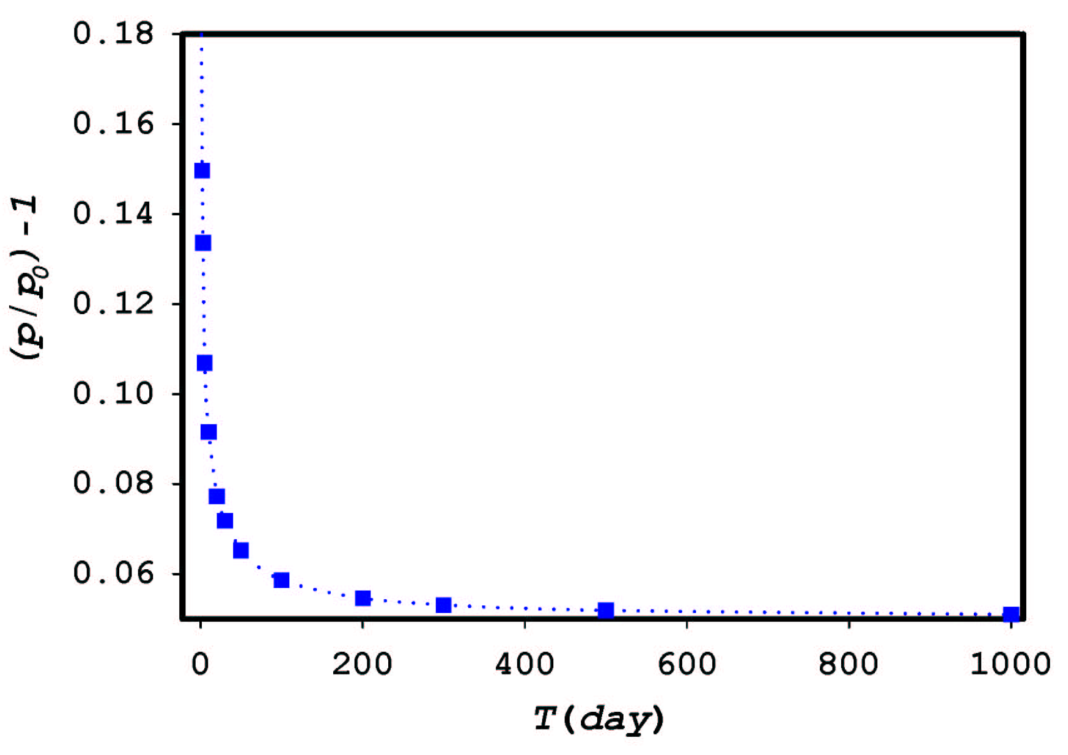
The relation between the loading parameter, (
p/p0) − 1, and the contract duration,
T , is plotted in
Figure 1. The loading parameter is used instead of premium to eliminate dependence of the premium on the monetary unit. It displays what we expected in real cases. Our usual trading experience tell us that a long term contract is more advantageous than some short term ones for a given period of time.
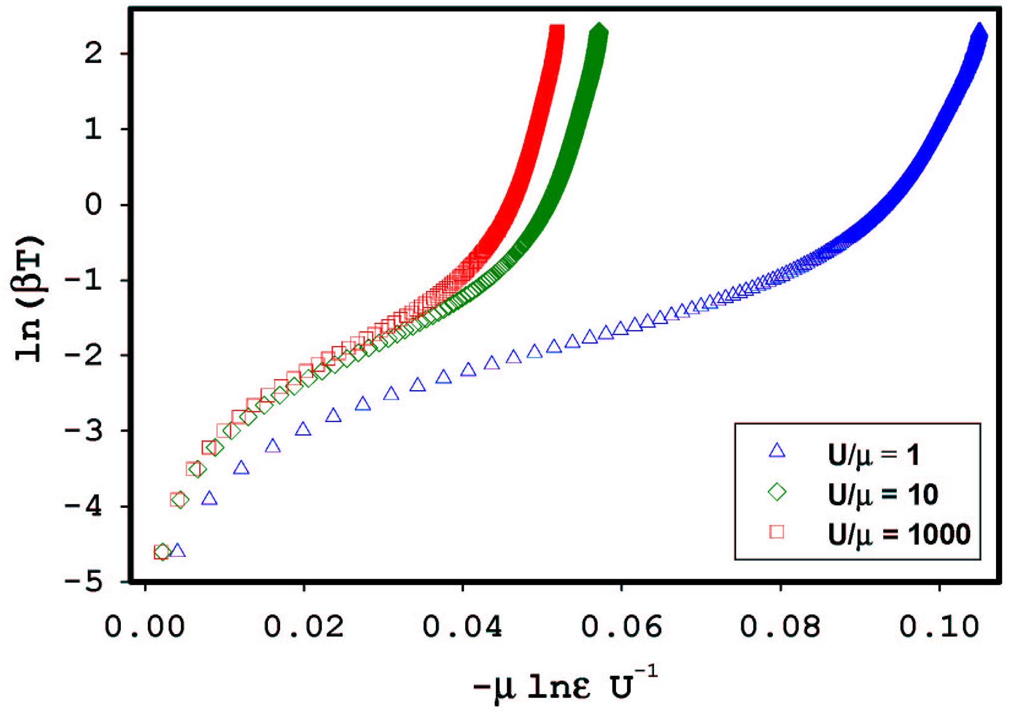
As we already mentioned, if we specify the ruin probability, the initial wealth and the mean claim size the
β parameter will be determined.
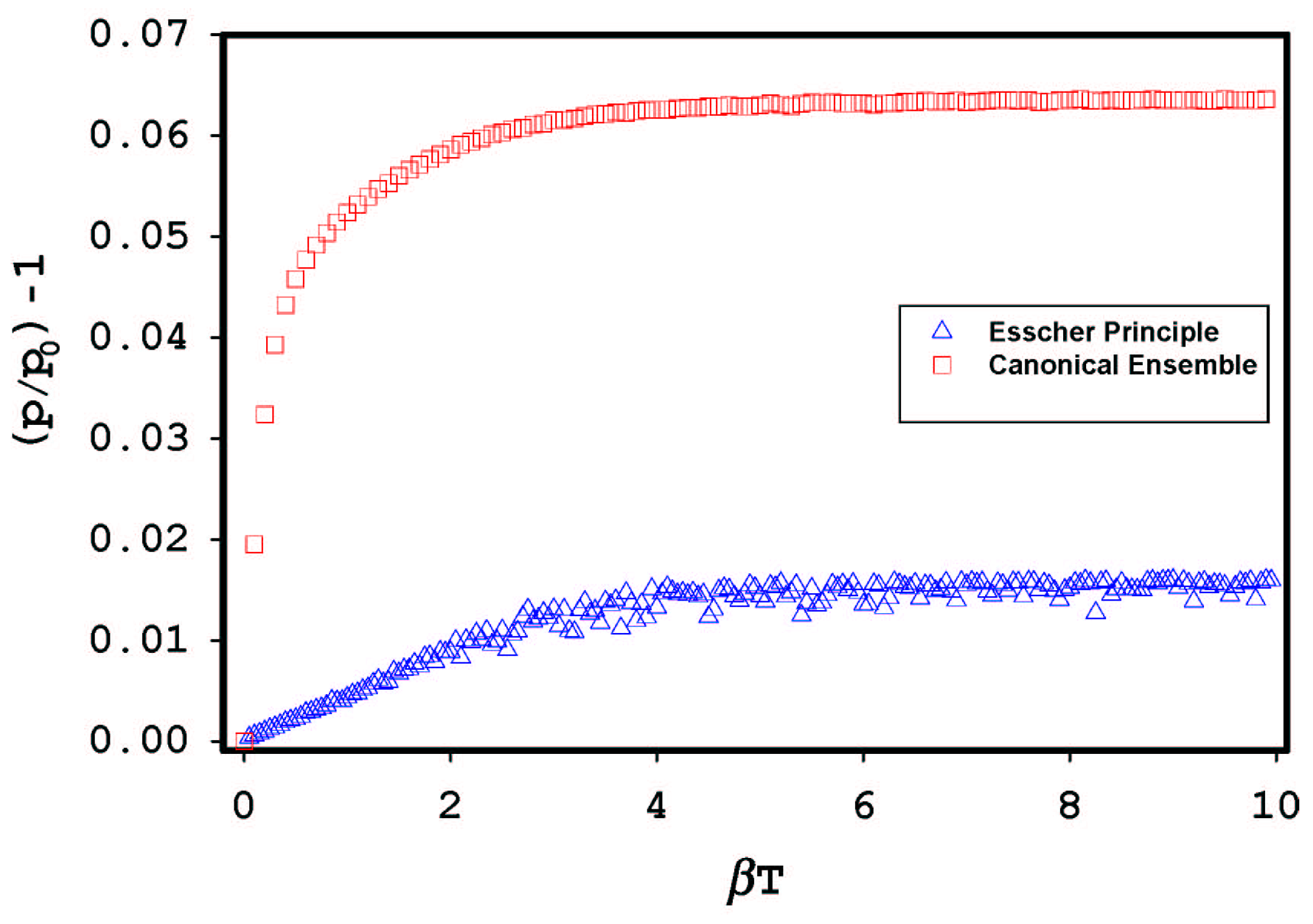
Figure 2 displays the relation between these parameters. The initial wealth is measured in terms of the mean claim size to avoid working with the monetary unit. The variation in number of the policy holders influences the premium.
Figure 3 is plotted to show this effect, the value of the premium which is obtained from Esscher formula is less than that we found in our method.


 in the derivation of above equality.
 is denoted by the symbol β, whence the condition for equilibrium becomes,
 when it is in equilibrium with its environment? From basic probability theory we know it should be directly proportional to the number of possible ways corresponding with the market state.

 is also much larger than
  hence the eq. 7 up to a constant coefficient; can be approximated as,


 , in accordance with their policies. The number of these claims is symbolized by Nα(T). The quantities, Iα(T),Nα(T) and
  are random variables.


