Markov Property and Operads

Abstract
:1 Introduction
2 Punctured random spheres and markov property

 depend smoothly on t. The Green kernel associated to the Hilbert structure (2) are the product of the one dimensional Green kernel es(s′)et(t′) = Es,t(s′, t′).
 and
and  are two R-valued independent Brownian motion. In the sequel, we will choose this procedure in order to construct the Brownian motion B1,u(S) with values in H1.
 . The Green kernel associated to this Hilbert space are of the type
 , associated to the Hilbert space H2 satisfy to

 (.) over H3. We multiply these Brownian motions by a deterministic function g(t) equal to 0 only at 0 and 1 such that g(1/2) (., 1/2) corresponds to a normalized circle of length 1. Outside these boundary tubes, we consider over the cylinder with constraint h(s1, 1) = h(s2, 1) = 0, a Brownian motion with values in H1, chosen independently of the others Brownian motions, but which intersect the input boundary tube on the cylinder S1 × [1 − ∊, 1]: we multiply by a smooth function g(t) > 0 which is 0 only in 1 − ∊. When the loop s → h(s, t) splits in two loops, we get two loops: we add the Brownian motion with values in H2 over each (Two independent one modulo some normalizing constants), and we get two cylinders which intersect the exit tube S1 × [0, 1/2] over the tube S1 × [0, ∊]. We mutiply these Brownian motion by a smooth function g(t) > 0, and which is 0 on ∊.
 (.) be d independent copies of Btot,..(S). We write
  . We consider the equation in Stratonovitch sense:

 (., t + 1/2) − (., t) and (., 1/2 − t′) − (., 1/2) are independent. The only problem in establishing the Markov property lies near the boundary. But if we we write


3 Line integrals


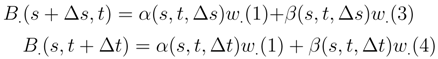
 , < w.(3), w.(2) >= O
  and that the correlator < w.(2),w.(4) >= O
  . We remark that
  .
.
 . We don’t write the analoguous expression for
  . There is a double integral in dw.(2) where the simple derivative of β(s,∆) in
  appear and a simple integral where the second derivative in of α(s, ∆s) and β(s,∆s) appear. (.) is the time of the differential equation (15). Moreover, in law:

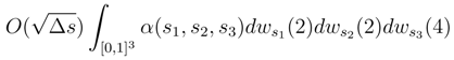
 and < w.(1),w.(4) >= O that the Itô integral which appears in the Clark-Ocone formula are in O dw.(2) and in O dw.(4). These leads to expressions of the type,
 . It is a smooth functional in the sense of Malliavin Calculus in w.(2), w.(4) and its derivatives
  have an estimate in O( )k
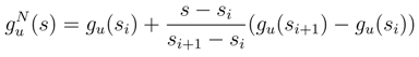
 is piecewise differentiable. We consider the random variable:

 :
:
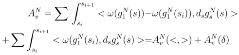 (δ) and the Stratonovitch counterterm is (<, >). The Itô term can be divided into two pieces: the first one is when in (30) we take the term in
  and the second one is when we take in (31) the term in
  . We get the decomposition, of the Itô term in
 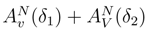 . The term which diverges ”a priori” is (δ1). But we can use (32), and show that when N → ∞,
 tends in L2 to a limit random variable called
  . Moreover, there exists a smooth version of the line integral Av in v.
 is the Bracket term
 is the Itô term:


 .
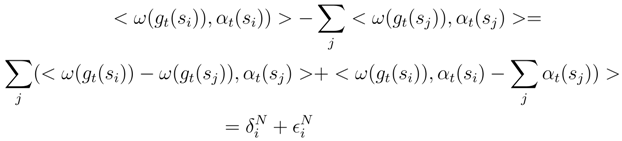
. whose writing is derived from (24) by taking another derivative, there is a linear integral which comes from the second derivative of α(si + ∆si), from a second derivative in β(s,∆s) in and a double integral which comes from taking only one derivative in β(s,∆s). The term in the linear integral can be treated in the following way: we get ∑
  . If M > N
 , we write si+1 − si = ∑sj+1 − sj such that we can write the sum to estimate

 is the term in the simple integral where we take the second derivatives in of α(s,∆s) and β(s,∆s). The terms which are integrated depend continuously from s. Therefore the contribution where we take two derivatives of α(s,∆s) vanish. It remains to consider the contribution where we take two derivatives of β(s,∆s). We can replace the terms considered by
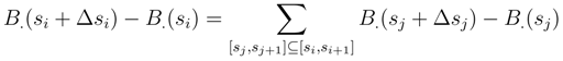
 . We write B.(s + ∆si) − B.(si) = ∑B.(sj + ∆sj) − B.(sj) and we see that < B.(sj + ∆sj) − B.(sj), B.(sj′ + ∆sj′) − B.(sj′) >= O(∆sj∆sj′) if j ≠ j′ and equal to O(∆sj)) if j = j′. This shows that the L2 norm of
 , we can assimilate
  with the double integral αu(si) after performing these replacements. Let N′ > N and sj be the dyadic subdivision which is associated. We sum over [sj, sj+1] ⊆ [si, si+1]. We get:
 . In the double integral which compose αt(si), we write
 into a finite variational part which converges by using (26) to 0 and a martingale part
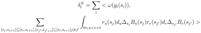
  . Namely, we can convert the double Stratonovitch integral which appears in (54) in an Itô integral. The boring term arises when we replace the double Stratonovitch integral by an Itô integral in (54). We would like to show that this martingale tends to 0. For that, we compute its quadratic variation. We get a sum over all quadruple [sj1, sj1+1], [sj2, sj2+1], [sj3, sj3+1] and [sj4, sj4+1].
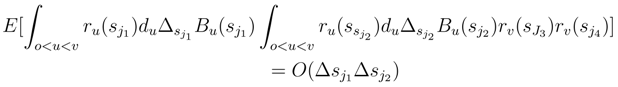
 are two independent Brownian motions. We can write At = WtVt where dVt = VtdBt and
  . after using this remark in order to calculate the conditional expectation, we desintegrate along ∆sj1B.(sj1) and ∆sj2B.(sj2) as in (32), and we conclude by using the consideration following (27), (28), (29). is a Cauchy sequence in L2.
 .
.
 in L2.
 for i ≠ i′. By (32),
 . By using the consideration of the first step, we can write modulo a term which vanish that

 and
and  . We deduce that < w.(5), w.(3) >= o(∆sj), < w.(5), w.(2) >=
  and < w.(5), w.(1) >= . In a similar way, we have < w.(3), w.(1) >= , < w.(3), w.(4) >= O(∆sj) (We used the fact that ∆sj = ∆sj′). With this decomposition, we write the analoguous of (30) and (3 1) for g.(sj + ∆sj) by doing the conditional expectation along the Gaussian processes w.(5),w.(4),w.(2),w.(3) and for g.(sj′ + ∆sj′). We find if j ≠ j′ and in the other cases
  . Therefore,
  .
.
 is
is
 . These expressions can be treated exactly as in the first step of the convergence of ∑ , by writing < , > as a double integral and relpacing (si+1 − si) < , > by a double stochastic integral where we have removed
  by ∆siB.(si). The sum of the others terms tends clearly to 0.
 has a smooth version, we show that the system of derivatives of in v converges in L2. We conclude by using the embedding Sobolev theorem as in [23].

 as in (35) with this new approximation. If we look the asymptotic expansion of FN, we see that the more singular term in
  and
and  coincides. This justify the following theorem: tends in L2 for the Ck topology over each compact of the parameter set to the Stratonovitch integral
  which has a smooth version in v.
4 Integral of a two form


 and the symmetric property.
 is
is
 tends for the Ck topology over each compact of the parameter space in L2 to the stochastic integral in Stratonovich sense:
 has a smooth version in v.
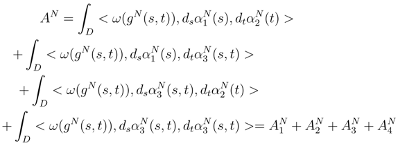
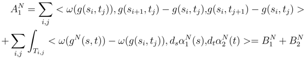
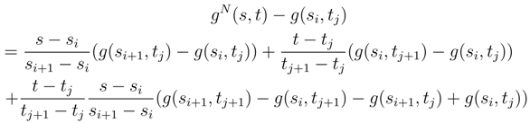
 . We repeat the considerations of the part III for s → B.(s, tj) and t → B.(si, t). If we fix tj, we get by (30) an asymptotic expansion in order 3. We get expressions in the asymptotic expansion in
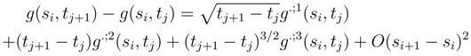
  and g3;.(si, tj). If we fix si, we go in (30) to an asymptotic expansion at order 3. We get derivatives in law
  .
.
 is the Itô term, which is apparently the most diverging when N → ∞.
  is the Stratonovitch counterterm..
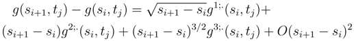
 and in
  which apparently do not converge and to integrals in (si+1 − si)g2;.(si, tj) as in (tj+1 − tj)g.;2(si, tj) which will lead to classical integrals. We deduce the following decomposition of the Itô term :

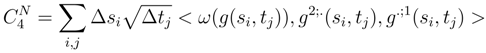
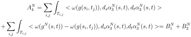
 is the double stochastic integral in the time direction s and in the time direction t:
 is a stochastic integral in the direction s and a classical integral in the direction t:

 is a vanishing term:
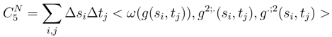
 is a classical integral in the time direction s and a stochastic integral in the time direction t:
 is a classical integral in the time direction s and in the time direction t.
 is the more ”a priori” divergent term when N tends to ∞ and will lead to a double classical integral on the torus.


 by (92). We get to take the expectation of the product of four Itô integral or 5 or 6. We can estimate its expectation by using the Itô formula and (93), (94) by applying iteratively the Itô formula and the Clark-Ocone formula. We reduce iteratively the length of the iterated integral we have to compute. The same result holds by the same arguments for:

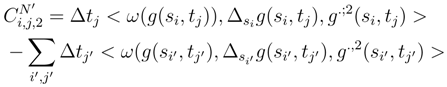
 tends to 0 when N′ → ∞. We will see later (See Step I.1.2, Step I.1.3 and Step I.1.4) that we can replace
  by ∆sig(si, tj) and
  by ∆tjg(si, tj). it is enough therefore to consider the behaviour of
 tends to 0.

 and ∆tjg(si′, tj) by
  and ∆tjg(si′, tj) by
  and ∆tjg(si, tj) by
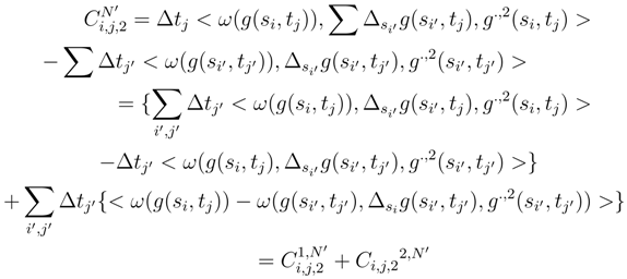
  . We get two quantities
  .
. . There are two contributions. The first one is when we consider twice the same si′. There are 4 types of increments which appear (si, tj), (si′, tj), (si, tj′ and (
  , tjj′). We take the conditional expectation along ∆si′B.(si′), tj), ∆tjB.(si, tj), ∆si′B(si′, tj′) and ∆tj′B(si, tj′) or more precisely along the Brownian motion which arise from the diagonalisation (89) of the Brownian motions B.(si, tj), B.(si′, tj), B.(si, tj′) and B.(si′, tj′). The Stratonovitch integrals g1;.(s, t) and g.;1(s, t) are in fact Itô integrals. Moreover we can compute the conditional law of g(si, tj), g(si′, tj), g(si, tj′) g(si′, tj′) by using (56) and the Clark -Ocone formula to express the quantities which appear in this way as stochastic integral which are martingales and whose bracket with the others tems can be estimated by (89). There is a product of Martingale Itô integrals, whose expectation can be estimated by using succesivly the Itô formula and the Clark Ocone formula. We conclude by using (4.27), (4.28) and (4.30). We get that the contribution when there is one coincidence leads to a term in O(1/N)∆si′∆tj∆tj′. When there is no coincidence, we condition by ∆si′B.(si′, tj), ∆tjB.(si, tj), ∆si”B.(si”, tj) and ∆tjB.(si, tj′) or more precisely by the Brownian motions arising from the diagonalisation (89). We proceed as before, and we get a contribution in
  .
. and after using the Clark-Ocone formula, we see that the quantity
  . The same holds for
  .
. . By the considerations which will follow in the next step, it is enough to study the behaviour of

 , we write:
 , we can replace
  . We can replace
  by
by  . We get
  and
and  .
. ,
,  . We can do the multiplication term by term in each product which appear. In each term, we distribute another time. There are 4 terms where two expressions in g1;. and g.;1 appear. We condition by the set of increments in the leading Brownian motion which appears in these expressions, or more precisely of the terms which appear after the diagonalisation (89) in ∆sB(s, t) and ∆tB(s, t). We use (57) and the Clark-Ocone formula (See [43]). We use (89), and (93). When we develop, there is the possibility that we get exactly 4 times si′, si”, tj′and tj”, which lead to a contribution in
  . There is a contribution when there are 3 different si, tj′, tj” or si′, si”, tj which lead to a contribution in
  and a contribution where we get only two times si and tj which leads to a contribution in
  tends to 0 in L2.
 tend to 0 in L2. By using this type of argument, we can get the requested limits. and where we mix stochastic integral and classical integral.


 , we can replace, by the considerations which will follow, ∆si′(g(si′, tj′) by the quantity
  . We get expressions
  and
and  . We distribute the term which appear in
  , there are 4 terms with increments
  which appear. We condition by the Brownian motions which are got after diagonalising the increments of the leadings Brownian motions which appear in these formulas and we get as before a norm in L2 which tends to 0.
 and the last one
  . The behaviour of
  is the most complicated to treat.
 and
and  as well as the sum where there exist other coincidences of indices i, i′, j, j′. We have to estimate the analoguous quantities where we mix
  and
and  , the term where we mix and and
  and the term where we mix and . We will omit to write the details of the convergence of these mixed term to 0. Clearly,

 and ∆tj2B(si2, tj2). Their mutual covariances satisfy to (92), (93) and (95) because j1 ≠ j2 and because we don’t have to consider when we do the multiplication term by term to consider the interaction between
  and the interaction between
  . We conclude after conditioning along these increments, or more precisely the Brownian motions which appear when we use the diagonalization (89). This allows us to show (114).
 , and the terms
  . We can apply (92), (93) and (95) to these increments because we don’t have to take the covariance between
  and the covariance between
  .
. because in g.;2(si′, tj) and in g.;2(si′, tj′) in (114), it is not the same subdivision in tj. But since we consider
 ,
,  and we don’t have to consider the correlation between
  and
and  and the correlation
  . We can apply (92), (93), (95) for the correlations we consider, and we can conclude as previously.
 , after doing the same restriction about the mixed terms. But as a matter of fact, we can show simply that
 ,
,  . But we have
  . Therefore:
 and because e has half derivatives in 0. This remark allows us to repeat the previous considerations as well as to use (92), (93) and (95).
 .
. , because two different subdivision [tj′, tj′+1] and [tj, tj+1] appear and because tj′ ∈ [tj, tj+1]. We write the details of this limit, because it is the most complicated, the others limits are simpler. We write:

 tend to 0. The main difficulty is to show that
 can be treated by Cauchy-Schwartz inequality. We proceed for that as it was done in the previous part. We remark, by the same considerations as in the first part, that it is enough to replace ∆tjg.;2(si′, tj) by a double stochastic iterated integral
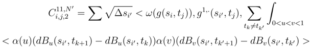
  dBv(si′, tj) where αu and αv are B(si′, tj) measurable. By the same argument, we replace ∆tj′g.;2(si′, tj′) by a double stochastic integral ∫0 < u < v < 1αu(si′, tj′)(dBu(si′, tj′+1) − dBu(si′, tj′)) αv(si′, tj′)(dBv(si′, tj′+1) − dBv(si′, tj′) where αu(si′, tj′) and αv(si′, tj′) are B.(si′, tj′) measurable. To study the behaviour when N! → ∞, we can replace without difficulty in this last expression αu(si′, tj′) by αu(si′, tj). We write:

 (We replace g(si, tj) by gr(si, tj), g1;.(si′, tj) by
  and the double integral between 0 and 1 by a double integral between 0 and r. Let us consider the finite variational part
  and the martingale part
  associated to this process.
 . This can come from a contraction between ω(g(si, tj)) and
  which leads to a term in
  , which is multiplied by a term in . But the L2 norm of the sum ∑tk≠tk′ can be estimated. We decompose first ∑tk≠tk in a martingale term and a finite variational term. There is first a contraction between αv and
  which leads to a term in tk′+1 − tk′ The stochastic integral in u can be estimated. We see the martingale term. By Itô formula
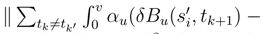
 can be estimated in
  . Therefore the L2 norm of this term behaves in
  . But since there is (tk′+1 − tk′) in time u, we have a behaviour of this contribution in ∆si(tj+1 − tj)3/2 whose sum vanish when N → ∞. The second term comes from a contraction between
  and which leads to a term in (tk+1 − tk)(tk′+1 − tk′) and therefore to a contribution in (tj+1 − tj)2. Therefore the total contribution is in ∆si(tj+1 − tj)2, whose sum vanish when N → ∞, because
  which is in (tk′+1 − tk′). This term cancel, because when we take the square of the L2 norm of the sum, it behaves in
 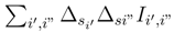 , where Ii′, i” where Ii′, i” is a sum of quadruple tk′, tk”, tk3, tk4 which behaves in O(tj+1 − tj)3 and a sum ∑i′∆siIi′ where Ii′ has a bound in tj+1 − tj)3/2. The sum of these terms vanish, when N → ∞ (See part III for analoguous considerations).
 . Let us estimate the L2 norm of
  . We use Itô formula. It behaves as
  where Ii′,i” has a bound in (tj+1 − tj)3/2 and Ii′ the same. Therefore the L2 norm of vanish when N → ∞.
 .
.


 in L2 because g2;2(si, tj) is bounded in L2.
 , we can replace ω(g(si′, tj′) by ω(g(si, tj)). We can replace ∆si′g2;.(si′, tj′) by a double stochastic integral in the dynamical time u I2;.(si′, tj′) as it was done in (126) and do the same transformation for the other g2;. and g.;2 which appear in such that we have only to show that
  in L2 where

 after distributing in these stochastic integral. Only the contribution where
  do not vanish when N′ → ∞, by the same considerations than in (54). These terms are nothing else, modulo some small error terms than I2;.(si′, tj) and I.;2(si, tj′). We have only to show that
  in L2 where
 .
. . But we have if si ≠ si′, by using the previous technics

 .
. .
.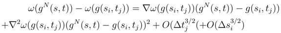
 lead to analoguous terms. If we consider the term where the square of gN(s, t)−g(si, tj) appear, there is a term where the quantity < ∇2ω(g(si, tj)); ∆sig(si, tj)2, ∆sig(si, tj), ∆tjg(si, tj) > appears whose sum vanishes in L2 by the same considerations as in Step I.1.4. The only problem comes when we take sum corresponding more and less to the double bracket of (s, t) → g1(s, t) of the type ∑i,j < ∇2ω(g(si, tj)).∆sig(si, tj).∆tig(si, tj), ∆sig(si, tj), ∆tig(si, tj) > whose treatment is similar to step I.1.3 by expanding a product of integrals into iterated integrals of length 2.
 and
and  . and are similar. So we will treat only the case of .
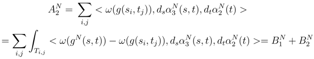 .
.
 can be treated as in step I.1. The term in
  can be treated as in step I.1, because the increments between ∆siB(si, tj) and ∆siB(si, tj+1) > satisfy to (121), and we can do as in the treatment of (121).
 .
. .
. + as
+ as  where
where
 .
.
 (s, t) of the random field g(s, t). As in the part III, the finite dimensional approximations of the integral
  will converge in L2, but we don’t know if they will converge to the same limit integral
  .
.


 (s, t), the more singular term is the same in (70), modulo some more regular terms which converge. The main Itô integral is the same, but we don’t know if the correcting terms are the same.
 converges in L2 to the stochastic Stratonovitch integral:
 has a smooth version in v.
5 Stochastic W.Z.N.W. model on the punctured sphere
 the stochastic 2-form:

 almost surely over
  .
.
 , with curvature
  for k an integer. Let us recall how to do (See [28], p 463-464): let gi be a countable system of finite energy loops in the group such that the ball of radius δ and center gi for the uniform norm Oi determine an open cover of L(G). We can suppose that δ is small. The loop gi constitutes a distinguished point in Oi. We construct if g belongs to Oi a distinguished curve joining g to gi, called l(gi, g): since δ is small, gi(s) and g(s) are joined by a unique geodesic for the group structure. lu(gi, g) is the loop s → expgi(s)[u(g(s) − gi(s))] where g(s) − gi(s) is the vector over the unique geodesic joining gi(s) to g(s) and exp the exponential of the Lie group associated to the canonical Riemannian structure over the Lie group. This allows to define over Oi a distinguished path joining g(.) to gi(.). We choose a deterministic path joining the unit loop e(.) to gi(.) li(e(.), gi(.)), and by concatenation of the two paths, we get a distinguished path joining g(.) to e(.) li(g(.), gi(.)) over Oi.
 which satisfies to our request and which is a stochastic plot. By pulling back (See [28], [30], [31]), we can consider the stochastic Z-valued form τst(ω) and integrate it over the surface . We put
 associated to the stochastic transgression τst(2πω) over
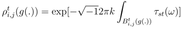
  is a collection of random variable
  measurables over Oj submitted to the rules
 of the line bundle
  is the space of measurable sections of such that
 over Oj, definition which is consistent, because
  is almost surely of modulus 1 in (159).
 . Moreover,
 by writting only L(G)), is given by:

 is a random one form over O given if u ∈ O by:
 the n output loop groups and
  the input loop group. We can define, by iterating, a generalization of the stochastic parallel transport, which applies a tensor product of sections
  over the output loop spaces to an element over the input loop space, because the different operations are compatible with the notion of glueing loops. We call this generalized parallel transport
  . It is not measurable with respect of the σ-algebras given by the restriction to the random 1 + n punctured to its boundary. Moreover, over each boundary, the laws of the loops are identical, and the Hilbert space of section of the bundle
  and ξin are identical. We denote it by Ξ. We consider the map τ1,n which associates to an element ξtot of the the tensor product of the Hilbert spaces of section at the exit boudary the section conditional expectation of ξtot with respect to the σ-algebra spanned by the input boudary. We get. :
References
- Airault, H.; Malliavin, P. Integration on loop groups; Publication Université Paris VI.: Paris, 1990. [Google Scholar]
- Albeverio, S.; Léandre, R.; Roeckner, M. Construction of a rotational invariant diffusion on the free loop space. C.R.A.S. 1993t, 316. Série I, 287–292. [Google Scholar]
- Arnaudon, M.; Paycha, S. Stochastic tools on Hilbert manifolds: interplay with geometry and physics. C.M.P. 1997, 197, 243–260. [Google Scholar] [CrossRef]
- Belopolskaya, Y.L.; Daletskiii, Y.L. Stochastic equations and differential geometry; Kluwer, 1990. [Google Scholar]
- Belopolskaya, Y.L.; Gliklikh, E. Stochastic process on group of diffeomorphism and description of viscous hydrodynamics. Preprint.
- Bismut, J.M. Mécanique aléatoire; Lect. Notes. Maths. 966; Springer: (Heidelberg), 1981. [Google Scholar]
- Brzezniak, Z.; Elworthy, K.D. Stochastic differential equations on Banach manifolds. Meth.Funct. Ana. Topo. 2000, (In honour of Y. Daletskii). 6.1, 43–84. [Google Scholar]
- Brzezniak, Z.; Léandre, R. Horizontal lift of an infinite dimensional diffusion. Potential Analysis 2000, 12, 249–280. [Google Scholar]
- Brzezniak, Z.; Léandre, R. Stochastic pants over a Riemannian manifold. Preprint.
- Chen, K.T. Iterated path integrals of differential forms and loop space homology. Ann. Maths. 1973, 97, 213–237. [Google Scholar]
- Daletskii, Y.L. Measures and stochastic equations on infinite-dimensional manifolds. In Espaces de lacets; Léandre, R., Paycha, S., Wurzbacher, T., Eds.; Public. Univ. Strasbourg: Strasbourg, 1996; pp. 45–52. [Google Scholar]
- Driver, B.; Roeckner, M. Construction of diffusion on path and loop spaces of compact Riemannian manifold. C.R.A.S. 1992, t 315, Série I, 603–608, (1992). [Google Scholar]
- Fang, S.; Zhang, T. Large deviation for the Brownian motion on a loop group. J. Theor. Probab. 2001, 14, 463–483. [Google Scholar] [CrossRef]
- Felder, G.; Gawedzki, K.; Kupiainen, A.Z. Spectra of Wess-Zumino-Witten model with arbitrary simple groups. C.M.P. 1988, 117, 127–159. [Google Scholar]
- Gawedzki, K. Conformal field theory. In Séminaire Bourbaki; Astérisque 177-178; S.M.F: Paris, 1989; pp. 95–126. [Google Scholar]
- Gawedzki, K. Conformal field theory: a case study. hep-th/9904145, (1999). [Google Scholar]
- Gawedzki, K. Lectures on conformal field theory. In Quantum fields and strings: a course for mathematicians; Amer. Math. Soci: Providence, 1999; Vol 1, pp. 727–805. [Google Scholar]
- Getzler, E. Batalin-Vilkovisky algebras and two-dimensional topological field theories. C.M.P 1994, 159, 265–285. [Google Scholar]
- Glimm, R.; Jaffe, A. Quantum physics: a functional point of view; Springer: Heidelberg, 1981. [Google Scholar]
- Gradinaru, M.; Russo, F.; Vallois, P. In preparation.
- Huang, Y.Z. Two dimensional conformal geometry and vertex operator algebra; Prog. Maths. 148; Birkhauser: Basel, 1997. [Google Scholar]
- Huang, Y.Z.; Lepowsky, Y. Vertex operator algebras and operads. In The Gelfand Mathematical Seminar. 1990-1992; Gelfand, I.M., Ed.; Birkhauser: Basel; pp. 145–163.
- Ikeda, N.; Watanabe, S. Stochastic differential equations and diffusion processes; NorthHolland: Amsterdam, 1981. [Google Scholar]
- Kimura, T.; Stasheff, J.; Voronov, A.A. An operad structure of moduli spaces and string theory. C.M.P. 1995, 171, 1–25. [Google Scholar] [CrossRef]
- Konno, H. Geometry of loop groups and Wess-Zumino-Witten models. In Symplectic geometry and quantization; Maeda, Y., Omori, H., Weinstein, A., Eds.; Contemp. Maths. 179; A.M.S.: Providence, 1994; pp. 136–160. [Google Scholar]
- Kunita, H. Stochastic flows and stochastic differential equations; Cambridge Univ. Press: Cambridge, 1990. [Google Scholar]
- Kuo, H.H. Diffusion and Brownian motion on infinite dimensional manifolds. Trans. Amer. Math. Soc. 1972, 159, 439–451. [Google Scholar]
- Léandre, R. String structure over the Brownian bridge. J. Maths. Phys. 1999, 40, 454–479. [Google Scholar]
- Léandre, R. Large deviations for non-linear random fields. Non. Lin. Phe. Comp. Syst. 2001, 4, 306–309. [Google Scholar]
- Léandre, R. Brownian motion and Deligne cohomology. Preprint. (2001). [Google Scholar]
- Léandre, R. Stochastic Wess-Zumino-Novikov-Witten model on the torus. J. Math. Phys. 2003, 44, 5530–5568. [Google Scholar]
- Léandre, R. Brownian cylinders and intersecting branes. In press. Rep. Math. Phys 2003. [Google Scholar]
- Léandre, R. Random fields and operads. Preprint. (2001). [Google Scholar]
- Léandre, R. Browder operations and heat kernel homology. In Differential geometry and its application; Krupka, D., Ed.; Silesian University Press: Opava, 2003; pp. 229–235. [Google Scholar]
- Léandre, R. Brownian surfaces with boundary and Deligne cohomology. In press. Rep. Math. Phys. 2003. [Google Scholar]
- Léandre, R. An example of a Brownian non-linear string theory. In Quantum limits to the second law; Sheehan, D., Ed.; A.I.P. proceedings 643; A.I.P.: New-York, 2002; pp. 489–494. [Google Scholar]
- Léandre, R. Super Brownian motion on a loop group. XXXIVth symposium of Math. Phys. of Torun.Mrugala, R., Ed.; Rep. Math. Phy2003; 51, 269–274. [Google Scholar]
- Loday, J.L. La renaissance des opérades. In Séminaire Bourbaki; Astérisque 237; S.M.F.: Paris, 1996; pp. 47–75. [Google Scholar]
- Loday, J.L.; Stasheff, J.; Voronov, A.A. Proceeedings of Renaissance Conferences; Cont. Maths. 202; A.M.S.: Providence, 1997. [Google Scholar]
- May, J.P. The geometry of iterated loop spaces; Lect. Notes. Maths. 271; Springer: Heidelberg, 1972. [Google Scholar]
- Mickelsson, J. Current algebras and group; Plenum Press: New-York, 1989. [Google Scholar]
- Nelson (Ed.) The free Markoff field. In J.F.A.; 1973; Volume 12, pp. 211–227.
- Nualart, D. Malliavin Calculus and related topics; Springer: Heidelberg, 1997. [Google Scholar]
- Pickrell, D. Invariant measures for unitary groups associated to Kac-Moody algebra; Mem. Amer. Maths. Soc. 693; A.M.S.: Providence, 2000. [Google Scholar]
- Pipiras, V.; Taqqu, M. Integration question related to fractional Brownian motion. Prob. Theo. Rel. Fields 2000, 118, 251–291. [Google Scholar] [CrossRef]
- Segal, G. Two dimensional conformal field theory and modular functors. In IX international congress of mathematical physics; Truman, A., Ed.; Hilger: Bristol, 1989; pp. 22–37. [Google Scholar]
- Souriau, J.M. Un algorithme générateur de structures quantiques. In Elie Cartan et les mathématiques d’aujourd’hui; Astérisque. S.M.F.: Paris, 1985; pp. 341–399. [Google Scholar]
- Symanzik, K. Euclidean quantum field theory. In Local quantum theory; Jost, R., Ed.; Acad. Press, 1989. [Google Scholar]
- Tsukada, H. String path integral relization of vertex operator algebras; Mem. Amer. Math. Soci. 444; A.M.S.: Providence, 1991. [Google Scholar]
©2004 by MDPI (http://www.mdpi.org). Reproduction for noncommercial purposes permitted.
Share and Cite
Léandre, R. Markov Property and Operads. Entropy 2004, 6, 180-215. https://doi.org/10.3390/e6010180
Léandre R. Markov Property and Operads. Entropy. 2004; 6(1):180-215. https://doi.org/10.3390/e6010180
Chicago/Turabian StyleLéandre, Rémi. 2004. "Markov Property and Operads" Entropy 6, no. 1: 180-215. https://doi.org/10.3390/e6010180
APA StyleLéandre, R. (2004). Markov Property and Operads. Entropy, 6(1), 180-215. https://doi.org/10.3390/e6010180