An Information Geometry-Based Track-Before-Detect Algorithm for Range-Azimuth Measurements in Radar Systems †


Abstract
1. Introduction
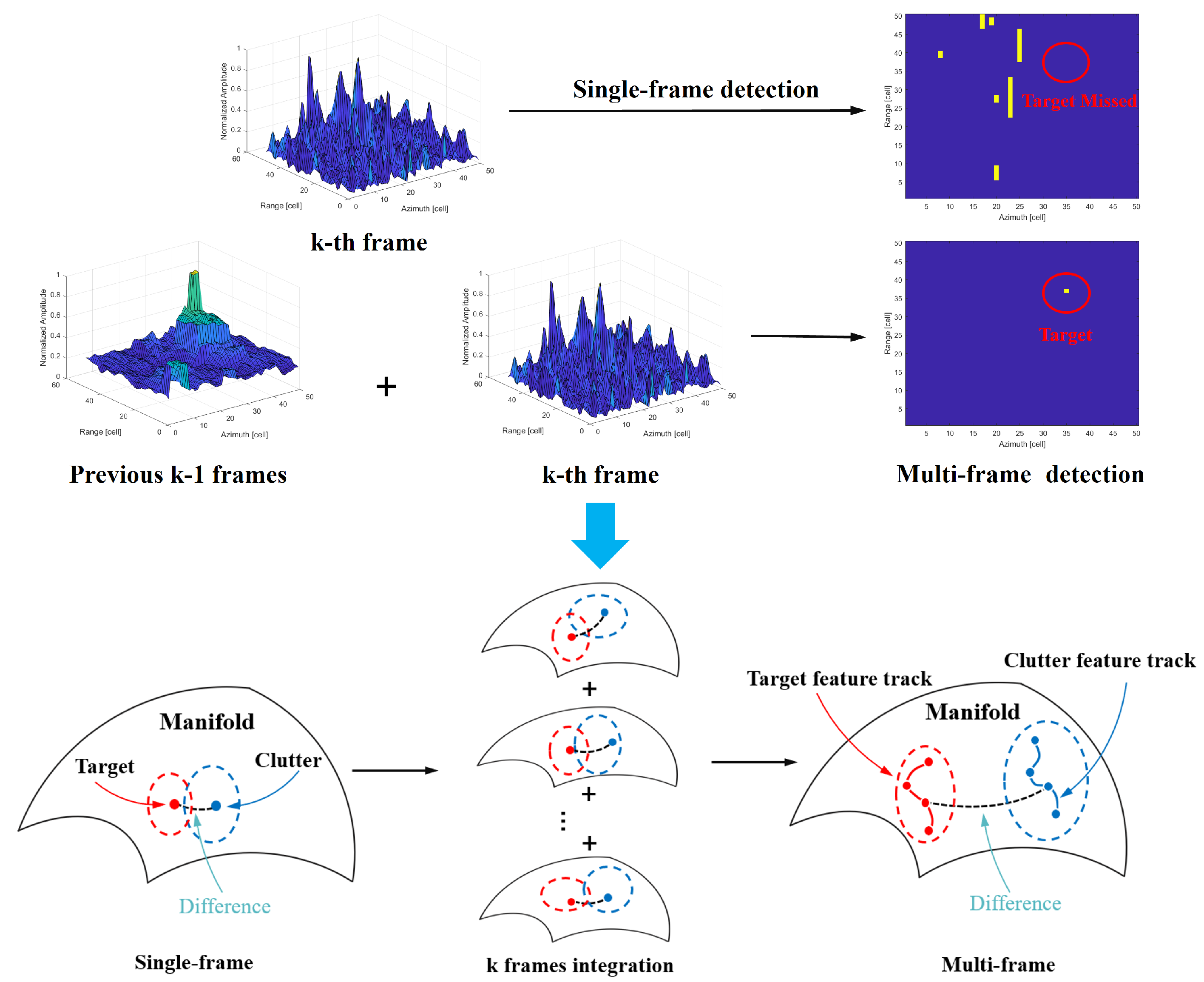
- IG-based inter-frame information integration for range-azimuth measurements: During the time interval between adjacent frames, the motion of the target induces changes in the features on the manifold. By analyzing the geometric properties of the target track and clutter track on the manifold, the information from range-azimuth measurements is integrated across multiple frames. Within the framework of information geometry detection, the target and clutter maintain distinguishability under multi-frame conditions. Meanwhile, the similarity between targets across frames introduces new information for integration.
- IG-based DP-TBD algorithm for range-azimuth measurements: Utilizing the distinctive features of targets and clutter on the manifold, a scoring function based on manifold distances is designed within the IG framework. An IG-based DP-TBD algorithm is derived to extract target trajectories that have the maximum integrated merit function values.
- Numerical experimental validation of real-recorded sea clutter data: Experiments using sea clutter data were performed to substantiate the effectiveness of the proposed methods. The findings confirm that these methods can accurately estimate target trajectories. Moreover, the detection performance of the proposed method provides at least a 3 dB improvement in SCR compared to traditional methods.
2. Problem Formulation and Preliminaries of IG Detector
2.1. Signal Model and Detection Model
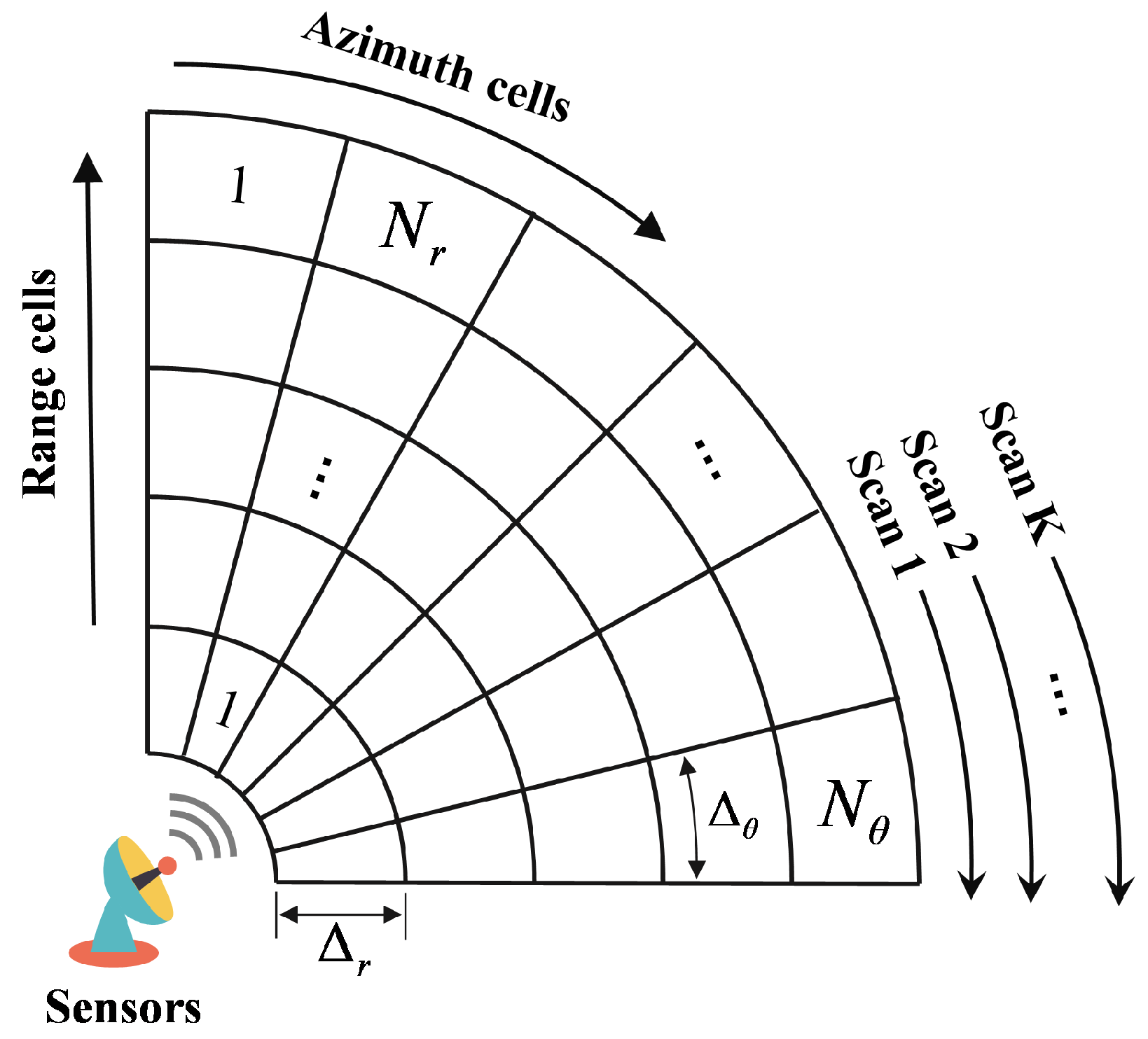
2.2. Measurement Model and Multi-Frame Detection Scheme
2.3. Information Geometry Detector
- , .
- if and only if .
3. IG-Based Track-Before-Detect Algorithm
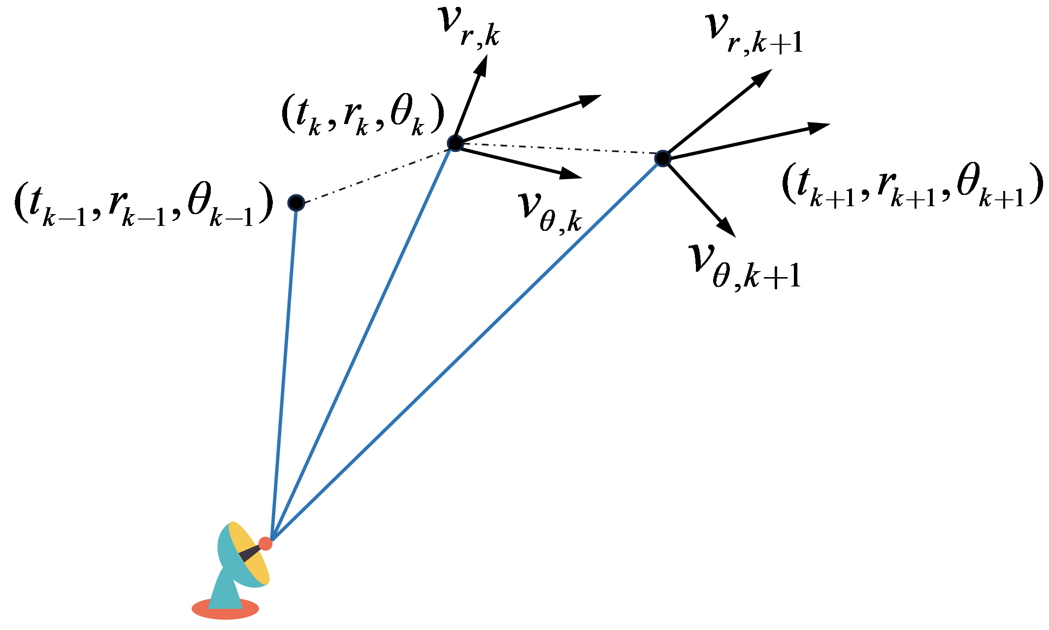
3.1. Kinematic Constraint for Trajectory of Moving Target
3.2. IG-Based Scoring Function
- (1)
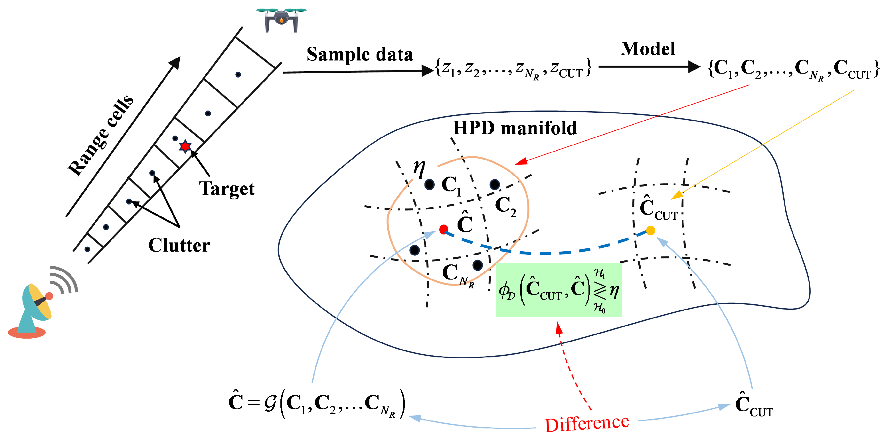
- For each frame , the distance between the target cells and clutter cells of the intra-frame should be as far as possible on the manifold, which is the dissimilarity in the Figure 6, i.e.,
- (2)
3.3. Multi-Frame Detection and Trajectory Estimate
| Algorithm 1: IG-based DP-TBD algorithm for range-azimuth Measurements |
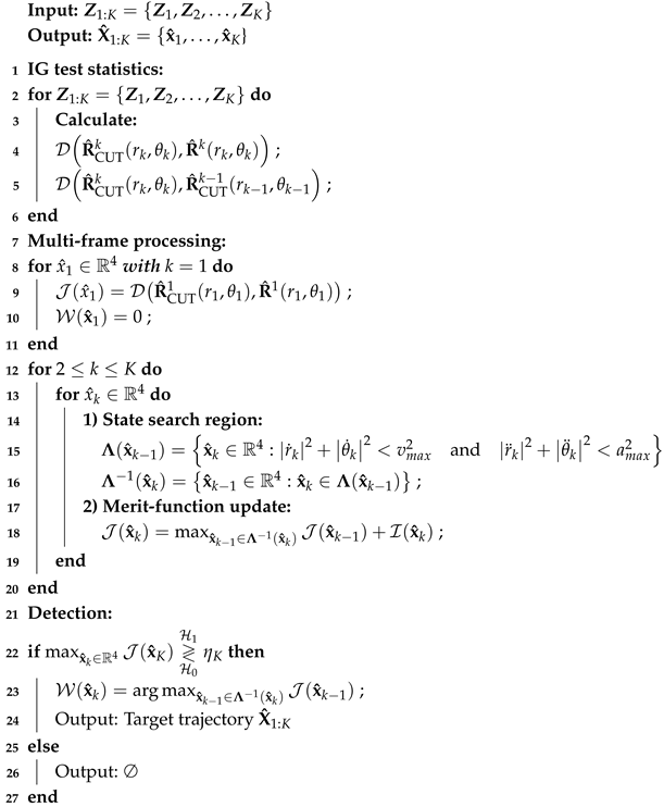 |
3.4. Computation Complexity
4. Experimental Results and Analysis
- Target detection probability : the maximum value of the IMF exceeds the detection threshold, while the discrepancy between the estimated and actual target position in the final frame is under two cells.
- Target track detection probability : the maximum value of the IMF exceeds the threshold, and the error of the estimated target trajectory compared with the real target trajectory is less than two cells within the whole track duration.
- Root Mean Square Error of Position : the average position error between the estimated trajectory and the real trajectory in the Cartesian Coordinate System.N denotes the number of Monte Carlo simulations.
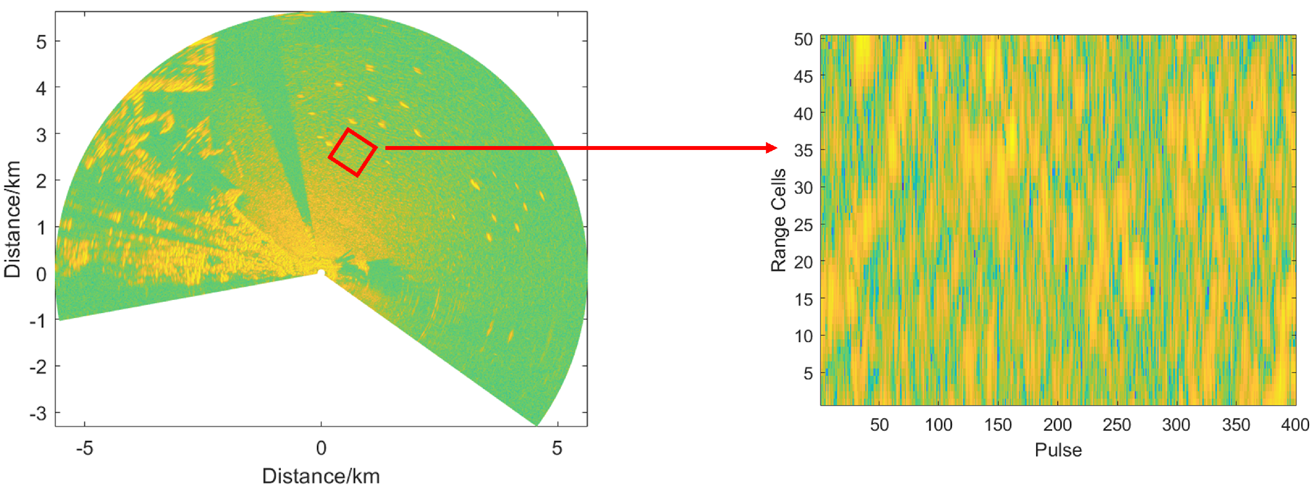
4.1. Real-Recorded Sea Clutter Data
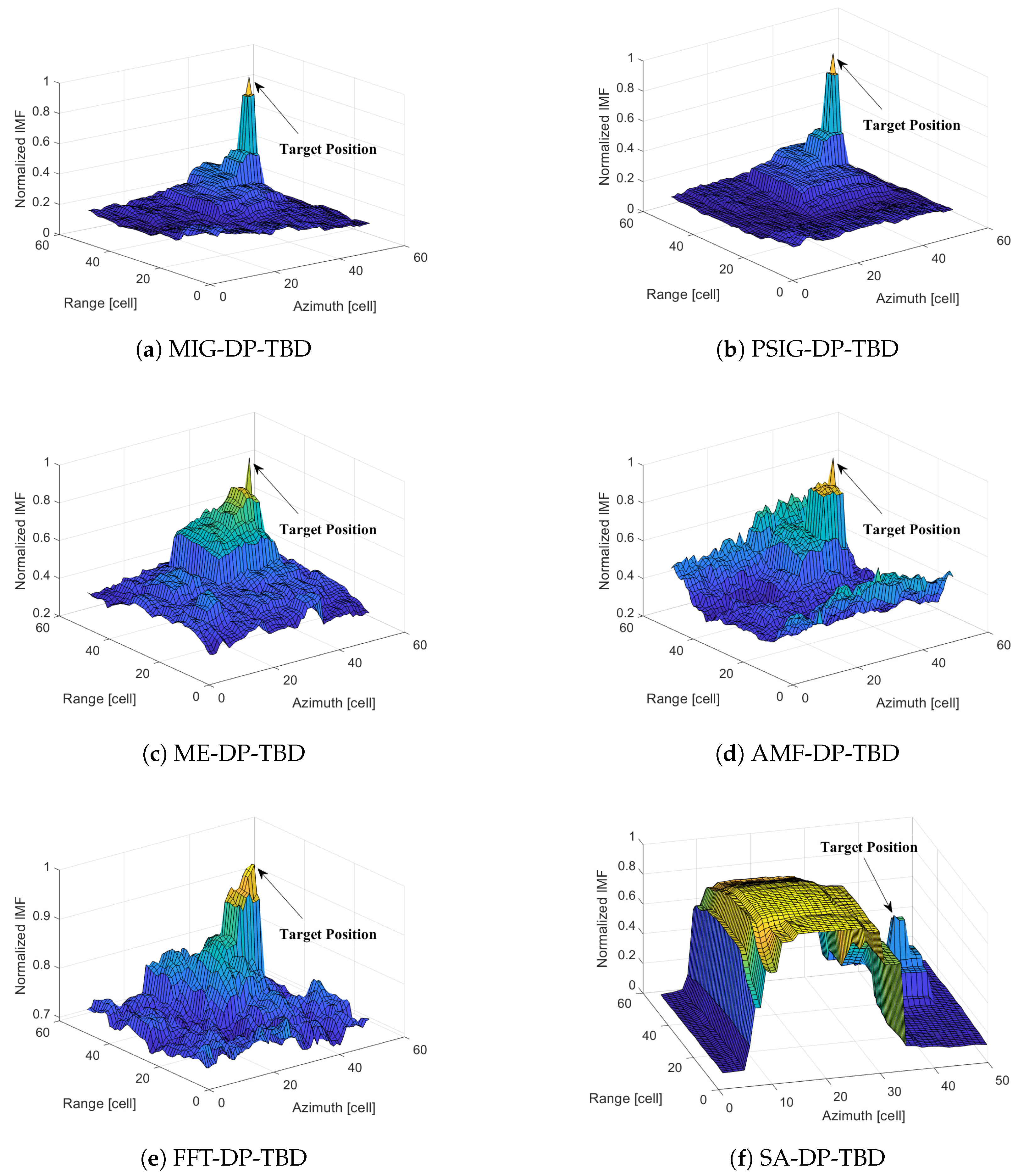
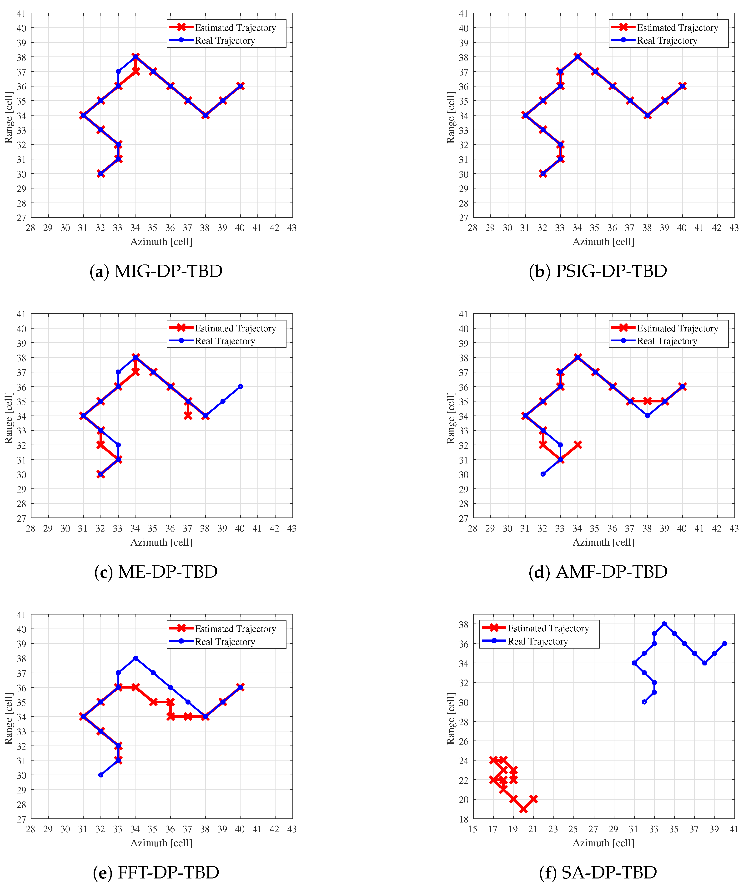
4.2. Comparison of Integration Merit Function and Trajectory Estimate
4.3. Comparison of Target Detection and Track Performance
5. Conclusions
Author Contributions
Funding
Institutional Review Board Statement
Data Availability Statement
Conflicts of Interest
References
- Coluccia, A.; Fascista, A.; Orlando, D.; Ricci, G. Adaptive Radar Detection in Heterogeneous Clutter Plus Thermal Noise via the Expectation-Maximization Algorithm. IEEE Trans. Aerosp. Electron. Syst. 2024, 60, 212–225. [Google Scholar] [CrossRef]
- Zhang, Y.; Li, Z.; Siddique, A.; Azeem, A.; Chen, W.; Cao, D. Infrared Small Target Detection Based on Interpretation Weighted Sparse Method. IEEE Trans. Geosci. Remote Sens. 2025, 63, 5001415. [Google Scholar] [CrossRef]
- Tang, M.; Aubry, A.; De Maio, A.; Rong, Y. Invariance Theory for Radar Detection in Disturbance With Kronecker Product Covariance Structure—Part I: Gaussian Environment. IEEE Trans. Signal Process. 2025, 73, 1577–1593. [Google Scholar] [CrossRef]
- Sahed, M.; Kenane, E.; Khalfa, A.; Djahli, F. Exact Closed-Form Pfa Expressions for CA- and GO-CFAR Detectors in Gamma-Distributed Radar Clutter. IEEE Trans. Aerosp. Electron. Syst. 2023, 59, 4674–4679. [Google Scholar] [CrossRef]
- Cai, J.; Hu, S.; Jin, Y.; Mo, J.; Yan, T.; Xia, M. A CA-CFAR-Like Detector Using the Gerschgorin Circle Theorem for Bistatic Space Based Radar. IEEE Trans. Aerosp. Electron. Syst. 2021, 57, 4137–4148. [Google Scholar] [CrossRef]
- Zhu, J.; Wen, C.; Duan, C.; Wang, W.; Yang, X. Radar Moving Target Detection Based on Small-Sample Transfer Learning and Attention Mechanism. Remote Sens. 2024, 16, 4325. [Google Scholar] [CrossRef]
- Kelly, E. An Adaptive Detection Algorithm. IEEE Trans. Aerosp. Electron. Syst. 1986, AES-22, 115–127. [Google Scholar] [CrossRef]
- Coluccia, A.; Fascista, A.; Ricci, G. Design of Customized Adaptive Radar Detectors in the CFAR Feature Plane. IEEE Trans. Signal Process. 2022, 70, 5133–5147. [Google Scholar] [CrossRef]
- Besson, O. Rao, Wald, and Gradient Tests for Adaptive Detection of Swerling I Targets. IEEE Trans. Signal Process. 2023, 71, 3043–3052. [Google Scholar] [CrossRef]
- Sun, M.; Liu, W.; Liu, J.; Hao, C. Rao and Wald Tests for Target Detection in Coherent Interference. IEEE Trans. Aerosp. Electron. Syst. 2022, 58, 1906–1921. [Google Scholar] [CrossRef]
- Du, X.; Jing, Y.; Chen, X.; Cui, G.; Zheng, J. Clutter Covariance Matrix Estimation via KA-SADMM for STAP. IEEE Geosci. Remote Sens. Lett. 2024, 21, 3507505. [Google Scholar] [CrossRef]
- Zhang, W.; An, R.; He, N.; He, Z.; Li, H. Reduced Dimension STAP Based on Sparse Recovery in Heterogeneous Clutter Environments. IEEE Trans. Aerosp. Electron. Syst. 2020, 56, 785–795. [Google Scholar] [CrossRef]
- Lapuyade-Lahorgue, J.; Barbaresco, F. Radar detection using Siegel distance between autoregressive processes, application to HF and X-band radar. In Proceedings of the 2008 IEEE Radar Conference, Rome, Italy, 26–30 May 2008; pp. 1–6. [Google Scholar] [CrossRef]
- Arnaudon, M.; Barbaresco, F.; Yang, L. Riemannian Medians and Means With Applications to Radar Signal Processing. IEEE J. Sel. Top. Signal Process. 2013, 7, 595–604. [Google Scholar] [CrossRef]
- Wu, H.; Cheng, Y.; Chen, X.; Li, X.; Wang, H. Adaptive Matrix Information Geometry Detector With Local Metric Tensor. IEEE Trans. Signal Process. 2022, 70, 3758–3773. [Google Scholar] [CrossRef]
- Yang, Z.; Cheng, Y.; Wu, H.; Liu, K.; Wang, H.; Qin, Y. Correlation-Feature-Based Information Geometry Detection for Weak Motion Target in Complex Environment. IEEE Internet Things J. 2025, 12, 11926–11939. [Google Scholar] [CrossRef]
- Yang, Z.; Cheng, Y.Q.; Wu, H.; Yang, Y.; Li, X.; Wang, H.Q. Adaptive Log-Euclidean Metric on HPD Manifold for Target Detection in Dynamically Changing Clutter Environments. IEEE Trans. Aerosp. Electron. Syst. 2024, 60, 9261–9274. [Google Scholar] [CrossRef]
- Zhao, W.; Liu, W.; Jin, M. Spectral Norm Based Mean Matrix Estimation and Its Application to Radar Target CFAR Detection. IEEE Trans. Signal Process. 2019, 67, 5746–5760. [Google Scholar] [CrossRef]
- Chen, X.; Wu, H.; Cheng, Y.; Feng, W.; Guo, Y. Joint Design of Transmit Sequence and Receive Filter Based on Riemannian Manifold of Gaussian Mixture Distribution for MIMO Radar. IEEE Trans. Geosci. Remote Sens. 2023, 61, 5102213. [Google Scholar] [CrossRef]
- Zou, R.; Cheng, Y.; Wu, H.; Yang, Z.; Liu, K.; Hua, X. A Two-Step Space-Time Adaptive Matrix Information Geometry Detector for Multi-Channel Radar. IEEE Trans. Aerosp. Electron. Syst. 2025, 1–13. [Google Scholar] [CrossRef]
- Yang, Z.; Cheng, Y.; Wu, H.; Li, X.; Wang, H. Manifold Projection-Based Subband Matrix Information Geometry Detection for Radar Targets in Sea Clutter. IEEE Trans. Geosci. Remote Sens. 2023, 61, 5110415. [Google Scholar] [CrossRef]
- Barbaresco, F.; Meier, U. Radar monitoring of a wake vortex: Electromagnetic reflection of wake turbulence in clear air. Comptes Rendus Phys. 2010, 11, 54–67. [Google Scholar] [CrossRef]
- Wu, H.; Cheng, Y.; Chen, X.; Yang, Z.; Liu, K.; Wang, H. Power Spectrum Information Geometry-Based Radar Target Detection in Heterogeneous Clutter. IEEE Trans. Geosci. Remote Sens. 2024, 62, 5102016. [Google Scholar] [CrossRef]
- Wen, L.; Ding, J.; Xu, Z. Multiframe Detection of Sea-Surface Small Target Using Deep Convolutional Neural Network. IEEE Trans. Geosci. Remote Sens. 2022, 60, 5107116. [Google Scholar] [CrossRef]
- Li, W.; Yi, W.; Teh, K.C.; Kong, L. Radar Multiframe Detection in a Complicated Multitarget Environment. IEEE Trans. Geosci. Remote Sens. 2023, 61, 5107516. [Google Scholar] [CrossRef]
- Rao, B.; Zhou, Y.; Nie, Y. Detection and Tracking of Weak Exoatmospheric Target with Elliptical Hough Transform. Remote Sens. 2022, 14, 491. [Google Scholar] [CrossRef]
- Kennedy, H.L. Efficient Velocity Filter Implementations for Dim Target Detection. IEEE Trans. Aerosp. Electron. Syst. 2011, 47, 2991–2999. [Google Scholar] [CrossRef]
- Ito, N.; Godsill, S. A Multi-Target Track-Before-Detect Particle Filter Using Superpositional Data in Non-Gaussian Noise. IEEE Signal Process. Lett. 2020, 27, 1075–1079. [Google Scholar] [CrossRef]
- Tian, M.; Chen, Z.; Wang, H.; Liu, L. An Intelligent Particle Filter for Infrared Dim Small Target Detection and Tracking. IEEE Trans. Aerosp. Electron. Syst. 2022, 58, 5318–5333. [Google Scholar] [CrossRef]
- Elhoshy, M.; Gebali, F.; Gulliver, T.A. Expanding Window Dynamic-Programming-Based Track-Before-Detect With Order Statistics in Weibull Distributed Clutter. IEEE Trans. Aerosp. Electron. Syst. 2020, 56, 2564–2575. [Google Scholar] [CrossRef]
- Rodriguez-Blanco, M.; Golikov, V. Multiframe GLRT-Based Adaptive Detection of Multipixel Targets on a Sea Surface. IEEE J. Sel. Top. Appl. Earth Obs. Remote Sens. 2016, 9, 5506–5512. [Google Scholar] [CrossRef]
- Cai, J.; Wang, R.; Li, M.; Liu, S.; Yan, Y.; Hu, C. An Efficient Threshold Determination Algorithm for DP-TBD Based on Structural Analogy and Saddle-Point Approximation. IEEE Trans. Aerosp. Electron. Syst. 2023, 59, 8263–8281. [Google Scholar] [CrossRef]
- Yang, Z.; Cheng, Y.; Wu, H.; Zou, R.; Hua, X.; Liu, K. Maximum Eigenvalue-Based Multi-Frame Track-Before-Detect Method for Weak Moving Target Detection. IEEE Trans. Aerosp. Electron. Syst. 2025, 1–11. [Google Scholar] [CrossRef]
- Li, W.; Miao, Q.; Yuan, Y.; Tian, Y.; Yi, W.; Teh, K.C. Automotive Radar Multi-Frame Track-Before-Detect Algorithm Considering Self-Positioning Errors. IEEE Trans. Intell. Transp. Syst. 2025, 1–16. [Google Scholar] [CrossRef]
- Zheng, S.; Li, D.; Yang, Q.; Zhao, Y.; Jiang, L.; Wang, Z. A Log-Normal Complex-Amplitude Likelihood Ratio-Based TBD Method With Soft Orbit-Information Constraints for Tracking Space Targets With Space-Based Radar. IEEE Trans. Radar Syst. 2025, 3, 467–482. [Google Scholar] [CrossRef]
- Li, W.; Yi, W.; Kong, L.; Teh, K.C. An Efficient Track-Before-Detect for Multi-PRF Radars With Range and Doppler Ambiguities. IEEE Trans. Aerosp. Electron. Syst. 2022, 58, 4083–4100. [Google Scholar] [CrossRef]
- Wu, H.; Cheng, Y.; Chen, X.; Yang, Z.; Li, X. Information Geometry-Based Track-Before-Detect Algorithm for Slow-Moving Fluctuating Target Detection. IEEE Trans. Signal Process. 2023, 71, 1833–1848. [Google Scholar] [CrossRef]
- Li, W.; Yi, W.; Teh, K.C.; Kong, L. Adaptive Multiframe Detection Algorithm With Range-Doppler-Azimuth Measurements. IEEE Trans. Geosci. Remote Sens. 2022, 60, 5119616. [Google Scholar] [CrossRef]
- Liu, J.; Wu, H.; Hua, X.; Cheng, Y.; Yang, Z.; Liu, K.; Wang, H. Information Geometry-Based Multi-Frame Track-Before-Detect Algorithm with Range-Azimuth Measurements. In Proceedings of the IET International Radar Conference 2025, Jiaxing, China, 21–23 November 2025. under review. [Google Scholar]
- Li, X.R.; Jilkov, V.P. Survey of maneuvering target tracking. Part I. Dynamic models. IEEE Trans. Aerosp. Electron. Syst. 2003, 39, 1333–1364. [Google Scholar] [CrossRef]
- Grossi, E.; Lops, M.; Venturino, L. A Novel Dynamic Programming Algorithm for Track-Before-Detect in Radar Systems. IEEE Trans. Signal Process. 2013, 61, 2608–2619. [Google Scholar] [CrossRef]
- Wang, J.; Yi, W.; Kirubarajan, T.; Kong, L. An Efficient Recursive Multiframe Track-Before-Detect Algorithm. IEEE Trans. Aerosp. Electron. Syst. 2018, 54, 190–204. [Google Scholar] [CrossRef]
- Liu, N.; Ding, H.; Huang, Y.; Dong, Y.; Wang, G.; Dong, K. Annual Progress of Sea-detecting X-band Radar and Data Acquisition Program. J. Radars 2021, 10, 173–182. [Google Scholar] [CrossRef]
- Liu, N.; Dong, Y.; Wang, G.; Ding, H.; Huang, Y.; Guan, J.; Chen, X.; He, Y. Sea-detecting X-band radar and data acquisition program. J. Radars 2019, 8, 656–667. [Google Scholar] [CrossRef]
- Zhang, J.; Li, Y.; Li, Q.; Xiao, W. Variance-Constrained Local-Global Modeling for Device-Free Localization Under Uncertainties. IEEE Trans. Ind. Inform. 2024, 20, 5229–5240. [Google Scholar] [CrossRef]
- Zhang, J.; Xue, J.; Li, Y.; Cotton, S.L. Leveraging Online Learning for Domain-Adaptation in Wi-Fi-based Device-Free Localization. IEEE Trans. Mob. Comput. 2025, 1–15. [Google Scholar] [CrossRef]


| Parameters | Values |
|---|---|
| Operating frequency band | X |
| Operating frequency range | 9.3∼9.5 GHz |
| Scanning bandwidth | 25 MHz |
| Range resolution | 6 m |
| Pulse repetition frequency | 1.525 kHz, 3 kHz |
| Peak transmit power | 50 W |
| Antenna length | 1.8 m |
| Antenna operating mode | Circular scan |
| Antenna polarization method | HH |
| Antenna horizontal beamwidth | 1.2° |
| Range sampling rate | 60 MHz |
Disclaimer/Publisher’s Note: The statements, opinions and data contained in all publications are solely those of the individual author(s) and contributor(s) and not of MDPI and/or the editor(s). MDPI and/or the editor(s) disclaim responsibility for any injury to people or property resulting from any ideas, methods, instructions or products referred to in the content. |
© 2025 by the authors. Licensee MDPI, Basel, Switzerland. This article is an open access article distributed under the terms and conditions of the Creative Commons Attribution (CC BY) license (https://creativecommons.org/licenses/by/4.0/).
Share and Cite
Liu, J.; Wu, H.; Yang, Z.; Hua, X.; Cheng, Y. An Information Geometry-Based Track-Before-Detect Algorithm for Range-Azimuth Measurements in Radar Systems. Entropy 2025, 27, 637. https://doi.org/10.3390/e27060637
Liu J, Wu H, Yang Z, Hua X, Cheng Y. An Information Geometry-Based Track-Before-Detect Algorithm for Range-Azimuth Measurements in Radar Systems. Entropy. 2025; 27(6):637. https://doi.org/10.3390/e27060637
Chicago/Turabian StyleLiu, Jinguo, Hao Wu, Zheng Yang, Xiaoqiang Hua, and Yongqiang Cheng. 2025. "An Information Geometry-Based Track-Before-Detect Algorithm for Range-Azimuth Measurements in Radar Systems" Entropy 27, no. 6: 637. https://doi.org/10.3390/e27060637
APA StyleLiu, J., Wu, H., Yang, Z., Hua, X., & Cheng, Y. (2025). An Information Geometry-Based Track-Before-Detect Algorithm for Range-Azimuth Measurements in Radar Systems. Entropy, 27(6), 637. https://doi.org/10.3390/e27060637