1. Introduction
The amount of data in need of storage continues to grow at an astonishing rate. The International Data Corporation (IDC) predicts that the Global Datasphere (the total amount of data created, captured, copied, and consumed globally) will grow from 149 zettabytes in 2024 [
1], to 181 zettabytes by the end of 2025 [
2,
3], and to an estimated 394 zettabytes in 2028 [
4] (a zettabyte equals
bytes). These developments may even be accelerated by the advancement of generative AI models. In view of these developments, the importance of efficient data storage management can hardly be underestimated. A major challenge is to devise storage technologies that are capable of handling these huge amounts of data in an efficient, reliable, and economically feasible way.
1.1. Distributed Storage Systems and Storage Codes
In modern storage systems, data storage is handled by a
Distributed Storage System (DSS). A DSS stores data across potentially unreliable storage units commonly referred to as
storage nodes, which are typically located in servers in data centers in widely different locations. Efficient update and repair mechanisms are critical for maintaining stability, especially during node failures [
5]. To handle the occasional loss of a storage node, the DSS employs
redundancy, in the form of a
storage code [
6,
7]. Often, a DSS simply employs
replication, where the storage code takes the form of a
repetition code. But nowadays, many storage systems such as Amazon S3 [
8]; Goole File System [
9] and its successor Colossus [
10]; Microsoft’s Azure [
11,
12,
13]; and Facebook’s storage systems [
14,
15], offer a storage mode involving a (non-trivial) erasure code. Especially for
cold data (data that remains unchanged, for example for archiving), but also for warm data (data that needs to be updated only occasionally), non-trivial erasure codes such as Reed–Solomon (RS) codes, Locally Repairable Codes (LRCs) or Regenerating Codes (RGCs) are considered or already applied [
7,
16]. For example, Microsoft Azure employs a Reed–Solomon code for archiving purposes [
11]. Hadoop implements various Reed–Solomon (RS) codes [
17,
18], and the implementation of other codes such as HTEC has been proposed, see, e.g., [
19]. The Redundant Array of Independent Disks (RAID) standard RAID-6 specifies the use of two-parity erasure codes, see, e.g., [
20]. Huawei OceanStor Dorado [
21,
22] employs Elastic EC, offering choice between replication and EC, for example RAID-TP (triple parity), and IBM Ceph also offers a choice of EC profiles [
23,
24] (see also [
25]). Several good overviews of modern storage codes and their performance are available, see for example [
16,
26,
27,
28,
29]. For a general and recent reference on storage systems, see [
30], and for an overview of Big–Data management, see [
31].
1.2. Node Repair
In the case of a lost node, the DSS uses the storage code to repair the damage. During repair, the DSS introduces a
replacement node (sometimes called a
newcomer node) into the system and downloads a small amount of data from some of the remaining nodes, referred to as the
helper nodes; the data obtained is then used to compute a block of replacement data that is to be placed on the replacement node. This process, commonly referred to as
node repair, comes in two variations. In the simplest repair mode, referred to as
exact repair (ER) [
32,
33], the data stored on the newcomer node is an
exact copy of the data stored on the lost node. A more subtle repair mode, first considered in [
6], is
functional repair (FR), where the replacement data need not be an exact copy of the lost data, but is designed to maintain the possibility of recovering the data that was originally stored, as well as to maintain the possibility for future repairs. An ER storage code can be thought of as an
erasure code that enables efficient repair. In contrast, an FR storage code can be seen as a
family of codes, all having the same parameters, where an erasure in a codeword from a code in the family is corrected into a codeword from possibly another code in the family [
29] (Section 3.1.1). We define and discuss
linear FR storage codes in detail in
Section 3, and describe an example in Example 1. For a formal definition of general FR storage codes, we refer to [
29] (Section 3.1.1).
1.3. Effectiveness of a Storage Code
Key considerations for measuring the effectiveness of a storage code are the
storage overhead and the
efficiency of the repair process. The storage overhead is determined by the fraction of
redundancy employed by the code, and is measured by the
rate of the code. Efficient repair, first of all, requires an easily implementable repair algorithm. Other important factors are the amount of data that needs to be transferred during repair, referred to as the
repair bandwidth, and the amount of
disk I/O, the number of times that a symbol is accessed on disk. In addition, it is desirable to limit the number of nodes that participate in the repair process, known as the
repair degree [
6] or
repair locality [
34,
35].
In general, the data that is transferred by a helper node during repair may be
computed from the available data symbols stored in that node. If each of the helper nodes simply transfers a
subset of the symbols stored in that node, then we speak of
help by transfer (HBT) [
26,
29]; if, in addition, no computations are done either at the newcomer node then we speak of
repair by transfer (RPT) [
36,
37]. We say that a storage code is an
optimal-access code if the number of symbols read at a helper node equals the number of symbols transferred by that node [
26,
29,
38].
1.4. Regenerating Codes and Locally Repairable Codes
Research into storage codes has diverged into two main directions. Regenerating codes (RGCs) investigate the possible trade-off between the storage capacity per node and the repair bandwidth (the total amount of data download during repair), which is determined by the cut-set bound [
6]. On the other hand, Locally Repairable Codes (LRCs) study the influence of the
repair degree, the number of helper nodes that may be contacted during node repair [
34,
35,
39]. A good overview of the different lines of research on codes for distributed storage and the obtained results can be found in [
40].
We first discuss an often-used model for storage codes, see, i.e., [
6,
26,
27,
29]. A
regenerating code (RGC) with parameters
is a code that allows for the storage of
m information symbols from some finite field
, in encoded form, onto
n storage nodes, each of which being capable of holding
data symbols from
. We will refer to
as the
storage capacity or the
subpacketization of a storage node. The parameter
k indicates that at all times, the original stored information can be recovered from the data stored on
any set of
k nodes. It is assumed that
k is the smallest integer with this property; since any set of
r nodes can repair all the remaining nodes, we then have
. Note that the
rate of the code is the fraction
of information per stored symbol. The resilience of the code is described in terms of a parameter
r, referred to as the
repair degree, and a parameter
, referred to as as the
transport capacity of the code. If a node fails, then a
replacement node is introduced into the system, which is then allowed to contact an
arbitrary subset of size
r of the remaining nodes, referred to as the set of
helper nodes. Each of the helper nodes is allowed to compute
data symbols, which are then sent to the new node, which uses this data to compute a
replacement block, again of size
. Therefore, the repair bandwidth
of a RGC satisfies
. It has been shown [
6] that the parameters of an RGC satisfy the
cut-set bound
Remarkably, the cut-set bound is independent of
n (but
n does influence the required field size
q for code construction). For fixed
m,
k, and
r, the equality case in (
1) takes the form of a piece-wise linear curve that represents the possible trade-off between the storage capacity
and the transport capacity
. Note that we have
(since
k nodes can recover the data) and
(since
r nodes can repair); the points on the curve where
with minimal
(so with
) and
with minimal
(so with
are referred to as the Minimum Storage Regenerating (MSR) and Minimum Bandwidth Regenerating (MBR) points, respectively. It is easily verified that the achievable region determined by (
1) is convex and has precisely
k extreme points (also referred to as
corner points), see
Figure 1. We review the cut-set bound in detail in
Section 4.
An
optimal RGC is an RGC with parameters that attain the cut-set bound (
1). It has been shown [
41] (Theorem 7) that the MSR and MBR points are the only corner points that can be achieved by exact-repair RGCs; indeed, the only points on the cut-set bound between the MSR and MBR points that can be achieved by ER RGCs are the MSR and MSB points, with the possible addition of a small line segment starting at the MSR point and not including the next corner point. In fact, it is conjectured that the achievable region for ER RGCs is described by the (identical) parameter sets of Cascade codes [
42] and Moulin codes [
43]. Conversely, it has been shown [
44] that every point on the cut-set bound is achievable by functional-repair RGCs; however, these codes are not (or not really) explicit, require a very large field size, and do not come with a repair algorithm. As far as we know, the only known explicit optimal FR RGCs are the partial exact-repair MSR codes with
from [
37], the explicit
HBT “FMSR” codes in [
45] (see also the “random” NCCloud HBT codes in [
46] and the non-explicit
MSR codes in [
47]), and the two explicit optimal FR RGCs from [
48] and from [
49,
50]. Therefore, it is of great interest to construct “simple” FR RGCs with a small field size, in corner points different from the MSR and MBR points.
A
Locally Repairable Code (LRC) also has parameters
, where
m,
n,
k,
, and
have the same meaning as for RGCs, but now we just require that repair of a failed node is always possible if we employ a
specific set of
r helper nodes (i.e., we are allowed to
choose the
r helpers). In [
51,
52] the maximal
rate of such codes (without any constraint on
k) was investigated, and in [
52], it was conjectured that for the case where
, the optimal rate is achieved by partitioning the
n storage nodes into
repair groups of size
and, within each repair group, using an
optimal RGC, so with
m attaining equality in (
1). This partly explains our interest in RGCs with these parameters in this paper. It is an interesting problem to investigate optimal codes for the case where
![Entropy 27 00376 i001]() n
n.
1.5. Our Contribution
Many existing storage codes employ MDS codes or, essentially,
arcs in projective geometry, in their construction. Some examples are the MBR exact-repair codes obtained by the matrix-product code construction in [
53], the MSR functional-repair codes in [
37] and in [
47], and the exact-repair Moulin codes in [
43]. In this paper, we use MDS codes to construct
explicit optimal linear RGCs with
,
, and with
an integer with
, so with
, which we refer to as
-regular codes. In fact, we show that the existence of
-regular storage codes is
equivalent to the existence of an
MDS code, so they can be realized over finite fields
with
, and even as binary codes if
. These codes come with a relatively simple repair method, and we show that, if desired, they allow for help-by-transfer (HBT) repair. The parameters of these codes achieve the
r extremal points of the achievable cut-set region for varying
. Note that by employing the obvious
space-sharing technique [
37], we can use the two storage codes in consecutive extremal points on the cut-set bound (
1) to also achieve the points between these extremal points. Our construction is based on what we call
-regular configurations, collections of
subspaces of dimension
in an ambient space of dimension
m with restricted sub-span dimensions (such configurations where called
-good in [
48] and [
49], see also [
51] (Example 3.3)).
The contents of this paper are organized as follows. In
Section 2, we introduce some notation and we recall various notions from coding theory, and in
Section 3, we review linear storage codes. We revisit the cut-set bound in
Section 4, where we also show that in optimal RGCs with
, no two nodes store identical information; in addition, we show that if
s an integer such that
, then any
nodes carry
independent information, that is, together they carry an amount of information equal to
. In addition, in the case where
, we derive an inequality that motivates our definition of
-regular configurations in
Section 5, where we also construct such configurations for all relevant parameters. The
-regular configurations with
,
, and
are called
-regular. In
Section 6, we investigate the structure of such configurations.
Section 7 contains our main results. Here, we show that the repair of a lost node in an
-regular coding state necessarily involves an MDS code, thus providing a lower bound for the size of the finite field for which an
-regular storage code can be constructed. Theorems 3 and 4 together demonstrate existence of
-regular codes for all feasible pairs
, and include precise and simple repair instructions for the corresponding codes. In
Section 8, we describe how to obtain smaller
-regular storage codes with extra symmetry, involving only
-regular configurations of a more restricted type. Finally, in
Section 9, we present some conclusions.
2. Notation and Preliminaries
For a positive integer n, we define . We write to denote the (unique) finite field of size q. For two vectors and in some vector space , and for a matrix with entries in , define the dot product ; define , where denotes the i-th row of ; and define , where denotes the j-th column of .
We define the span of subspaces of an ambient vector space V as the collection of all sums with for . (In other works, the span is sometimes denoted as .) We simply denote the span of the vectors in V by . We say that subspaces of a vector space V are independent if , where denotes the dimension of a vector space V.
We repeatedly use
Grassmann’s identity, which states that for vector spaces
we have
We need various notions from coding theory. For reference, see, e.g., [
54].
The support of a vector is the collection of positions for which ; the (Hamming) weight of is the number of positions for which , that is, . The (Hamming) distance between is the number of positions for which . Note that .
A code C of length n over is just a subset of ; the code C is called linear if C is a subspace of . We often refer to the vectors contained in a code as codewords. The minimum weight of a code C is the smallest weight of a nonzero codeword from C, and the minimum distance of C is the smallest distance between two distinct codewords from C. Note that if the code C is linear, then . We often refer to a linear code C of length n, dimension k, and minimum distance d over as an code or as an code; we simply write or if the intended field is clear from the context.
A
generator matrix for an
code
C is a
matrix
over
with rank
k and with its rowspace equal to
C, that is,
C consists of the vectors
with
. An
matrix
is a
parity-check matrix for
C if
has rank
and
if and only if
. The
dual code
of
C is the collection of all vectors
for which
for all
. It is not difficult to see that
is an
-code, and has generator matrix
and parity-check matrix
, see also [
54] (Chapter 11).
Finally, we need some notions related to MDS codes. As a general reference for this material, see [
54] (Chapter 11). The
Singleton bound states that an
code satisfies
. For a proof, see, e.g., [
54] (Chapter 1, Theorem 11), or see [
55] (Theorem 4.1) for a generalization for non-linear codes. An
code, that is, a linear code that attains the Singleton bound, is called an
MDS code. A related notion is that of an
arc, a collection of nonzero vectors in
with the property that any
k of them are independent. (Usually, an arc is defined
projectively, that is, as a set of points in
, but for our purposes, this will do.) We say that a
matrix
represents an
n-arc if the columns of
constitute an
n-arc (i.e., an arc of size
n) in
; alternatively, we refer to such a matrix as an
MDS-generator. (The term
MDS matrix comes from cryptography and is commonly reserved for a matrix
M for which
is an MDS-generator.) Consider an
code
C, with generator matrix
and parity-check matrix
. Obviously, if
has
columns that are dependent, then
C has a nonzero codeword of weight at most
. Therefore,
C is MDS if and only if the columns of
form an
n-arc. Moreover, if
has
k columns that are dependent, then there exists
with
such that the codeword
is nonzero but has a 0 in the corresponding positions, so that
and
C is not MDS. Hence,
C is MDS if and only if
is an
n-arc, that is, if and only if its generator matrix (or parity-check matrix) is an MDS-generator. In particular,
C is MDS if and only if
is MDS [
56] and [
57] (Lemma 6.7, p. 245).
Note that
itself, the repetition codes with parameters
and their duals, the codes with parameters
(called even-weight codes when
), are all MDS codes. For
, let
denote the largest
n for which an
MDS code exists. The famous MDS conjecture, proven by Simeon Ball for the case where
q is prime in [
58], claims that
except that when
q is even,
For
, it was shown in [
59] that
, and that an
MDS code is equivalent to the dual of the repetition code, see also [
54] (Corollary 7). It is well known that
is at least equal to the stated values in (
2) and (
3). Indeed, we already mentioned that
is an MDS-generator for all
k; the corresponding linear code for
is called the
even-weight code. Furthermore, let
be the non-zero elements of
. If
, then
is a
MDS-generator; moreover, if
q is even, then
is a
MDS-generator. The corresponding codes are referred to as
(Generalized) Reed–Solomon codes. In fact, for any
k,
, such that
q is even or
k is odd, there exists a
cyclic MDS code over
[
60] (this corrects an erroneous claim in [
54]). For a reference for the above claims, see, e.g., [
54] (Chapter 11, Sections 5–7).
3. Linear Storage Codes
In this paper, we adhere to the
vector space view ([
33,
41,
48,
51,
53,
61,
62,
63]) on linear storage codes. Informally, a storage code with symbol alphabet
is called
linear if the four processes of data storage, data recovery, the generation of repair data from the helper nodes, and the generation of the replacement data from the repair data, are all linear operations over
[
29]. It turns out that in that case, the storage code can be described in terms of subspaces of an ambient vector space over
referred to as the
message space. In the description below, we will follow a similar approach as in [
49,
50]. We first need a few definitions.
Definition 1. We say that the subspaces of a vector space V form a recovery set for V if .
Definition 2. We say that a subspace of a vector space V can be obtained from subspaces of V by -repair
, written asif there are β-dimensional helper
subspaces () such that . We can now present a formal definition of a Linear Regenerating Code (LRGC) in terms of vector spaces, which can be seen as a “basis-free” representation of a linear storage code. To understand the definition, think of the data that is stored by the storage code as being represented by a vector in the ambient vector space , referred to as the message space of the code. Then for every subspace W of V that occurs in the definition, choose a fixed basis , and think of W as representing the t data symbols .
Definition 3. Let be integers for which and . A linear storage code with parameters consists of an ambient m-dimensional vector space V over together with a collection of sequences of α-dimensional subspaces of V, referred to as coding states of the storage code, with the following properties.
(i) (Data recovery) Every k subspaces in a coding state constitute a recovery set for V. Moreover, we will assume that k is minimal with respect to this property.
(ii) (Repair) For every and for every with , there is a subspace of V such that for which is again a coding state in .
For future use, we introduce some additional terminology.
Definition 4. We refer to the collection of all the α-dimensional subspaces of V that occur in some coding state in as the coding spaces of the linear storage code .
A subsequence ( of a state will be referred to as a protostate of the storage code .
So to actually employ the collection
as in Definition 3 as a storage code, think of the stored data as a vector
(or as a
linear functional, that is, as an element of the
dual of
V mapping
to
as in [
64]). Then, for every coding space
U involved in
, choose a
fixed matrix
with columnspace equal to
U; now, if
U is the coding space associated with a particular storage node, then we let this node store the
symbols of the vector
. Note that if
is any vector in
U, with
, say, then
, so for every
, we can compute
from the stored vector
. Similarly, for a repair subspace
H contained in a helper node with associated coding space
U during repair, we choose a fixed
matrix
with columnspace equal to
H, and let this (helper) node contribute the
symbols
. The
code associated with a coding state
is the collection
of all words
in
obtained as the concatenation of the words
for
when
ranges over
V. Note that
is an
code with
generator matrix
where
is a matrix with columnspace
, for all
i. It is not difficult to verify that the family of codes
associated with states
from a storage code
as in Definition 3 indeed has the desired repair properties when used in this way to store data. Note that the resulting functional-repair (FR) storage code is exact-repair precisely when the code consists of a
single coding state. In the case where the storage code is FR, at any time every storage node must “know” its associated coding space. The extra overhead that this entails can be relatively small if the code is used to store a
large number of data vectors
simultaneously. For further details, we refer to [
49,
50]. The next example illustrates the above.
Example 1 (See also [
48] (Example 2.2), [
49] (Example 2.6), and [
50] (Example 2.7))
. We will construct a binary linear functional-repair storage code with parameters (representing the smallest non-MSR/MBR extreme point of the achievable cut-set region). So let V be a 5-dimensional vector space over . A set of three 2-dimensional subspaces of V is said to be -regular
if any two of them are independent and (this was called -good
in the cited papers). It is easily verified that if is -regular, then there are nonzero vectors () such that ; as a consequence, there is a basis for V such that (). It is easily checked that with , any subset of of size 3 is -regular. As a consequence, the collection of all states for which any set of three of the spaces form a -regular collection is a linear storage code with the parameters as specified. Note that there are coding states that are unreachable
, that is, not obtainable by repair from a protostate; for example, states of the form with () and with ; obviously, such states can be freely deleted from the code. 4. The Cut-Set Bound Revisited
Suppose that the DSS employs an storage code. Since k is assumed to be minimal and any r nodes can regenerate the stored information, we have . (Indeed, to see this, choose an arbitrary set of r helper nodes, and one by one destroy and repair all the other nodes, employing these helper nodes for each repair. Then the information contained in the system is just the information that is contained in these r helper nodes.) Note also that, obviously, (since any k nodes regenerate the stored information), and (since r helper nodes, each contributing an amount of information, can create a replacement node), and (since is the maximum amount that can be contributed by a helper node). Finally, let s be an integer such that , or such that if ; therefore, we may assume that . We let and denote the normalized storage capacity and transport capacity, respectively. Our aim is to provide a quick and informal derivation of the cut-set bound for RGCs and to establish a few simple properties of optimal codes that seem to have gone unobserved. First, we show the following.
Lemma 1 (Cut-set bound
). Let be positive integers with , and let be positive real numbers with . Let s be an integer such that if or such that if . A storage code with parameters satisfies Moreover, in the case of equality in (7), we have the following. Any nodes, together, contain an amount of information , that is, these nodes carry independent information.
Any two nodes carry an amount of information of at least if or if . Therefore, if , then every node carries the stored information, so the code is essentially a repetition code, but if , then no two nodes carry identical information .
If, in addition, we have , then for any with size , the information contained in any collection of storage nodes with satisfiesif , andif with .
Proof. Assume that nodes
store the file, and that each
k nodes regenerate the stored file, with every node storing
symbols. Consider nodes
. Pretend that nodes
fail in turn, and are replaced by newcomer nodes
, with none of the nodes
ever participating in a repair. Assume that for
, the lost node
is replaced by newcomer node
, which receives an amount of
information from each node contained in the set of
r helper nodes consisting of the old nodes
, the new nodes
, and the old nodes
. Now consider the sequence
of
k nodes defined by
. The first
nodes
in
contain an amount of information that is at most equal to
. And for
, the information in
that is not already contained in the preceding nodes
in
is the information obtained from
, so is at most equal to
. As a consequence, the amount of information contained in
is at most equal to
, and since any
k nodes should be able to regenerate the stored information, we conclude that (
7) holds. Moreover, we conclude that if the bound (
7) holds with equality, then the nodes
in
, together, contain an amount of
of information, and, in addition, a node
contributes a further amount
of information that is independent of the information already present in preceding nodes in
.
By keeping track which of the nodes among contributed the various pieces of information during the above repair process, we see that node for contributes an independent amount of information , and the nodes each contribute an independent amount . Also note that the sequence of nodes , as well as their order, is arbitrary, and nodes and form an arbitrary pair of nodes. Now, if , then and we already showed that any nodes, together, contain at least an amount of of information; and if then nodes and , together, contain at least an amount of of information. Obviously, in the case where , every node carries the same information, so the code is essentially a repetition code. Finally, in the case where , by considering the sequence of nodes , we see that the last claim in the lemma holds. □
Definition 5. We say that a Regenerating Code (RGC) with parameters is optimal
if the bound (1) is attained with equality, and if, moreover, lowering α or β results in violation of this bound. Note that if
, then (
7) reads as
. In that case, if the code is optimal, then according to Definition 5, we must have
and
.
It is not difficult to see that in terms of the normalized parameters
and
, we have the following. For
, define
and set
Then the
feasible cut-set region, the region of all pairs
that can be realized by tuples
for which
,
, and for which (
7) holds with
s as defined above, has extreme points
for
, and is further bounded by the half-lines
and
, see
Figure 1 in
Section 1.
We sometimes refer to the extreme points () as the corner points of the achievable region. The corner points and are known as the MSR point and the MBR point, respectively (note that these points are equal if and only if ).
Definition 6. We say that an RGC with parameters attains a corner point of the achievable cut-set region if the pair equals one of the pairs with . An RGC that attains the MSR point or the MBR point is referred to as an MSR code or an MBR code, respectively.
Remark 1. The result in (9) may well hold also for optimal storage codes where , but we have no proof and no counterexample. Remark 2. There are cases of optimal codes where (9) is not satisfied with equality. Consider an MBR code with , , and . The “standard” code has coding spaces , where the vectors with form a basis. This code satisfies (8) and (9) with equality. Now, let , , , and . Note that can be obtained by repair from (use ), (use ), and (use ). Now any two coding spaces span at least a 5-space, and any three span a 6-space, but are independent.
This example shows that in a coding state, (9) is not necessarily satisfied with equality. But note that this example can only represent an unreachable
state in a storage code with these parameters, since once we have a protostate with no two spaces disjoint, then the new space has a repair vector in common with each of the other coding spaces. 5. -Regular Configurations
In this section, let
be integers with
, let
s be an integer with
, and let
be as defined in (
10). Moreover, let
be a positive integer and let
. Motivated by the results from the previous section—notably, by (
8) and (
9))—and by the form of the “small” storage codes from [
48,
49]) (see also [
50]), we introduce and investigate the following notion.
Definition 7. Let V be a vector space with , and let be α-dimensional subspaces of V. We say that the collection is -regular
in V if and, for every integer t with and for every with , we have , where In addition, we say that is -regular
if it is -regular with , and -regular if it is -regular with . We will write to denote the dimension of the ambient space of an -regular collection. Note that Definition 7 requires, in particular, that any
of the vector spaces in a
-regular collection are independent, and that any
k of the vector spaces span
V. Our aim in the remainder of this section is to study the properties of the numbers
defined in (
10), and to describe a construction of
-regular collections (and, hence, of
-regular configurations for all integers
). To that end, we need the following.
Lemma 2. For , define . Then . Let t be an integer with , and set . Then and In particular, for as defined in (10), we have Proof. Since
, we have
, hence
. Also,
. Obviously,
if
. Therefore, the first claim follows immediately. Since
, we have
, so we have
Taking , we have for all i, and we find that . □
Now, to construct a -regular configuration of size , we proceed as follows. For , let be a MDS-generator over a sufficiently large field , and let . Now let , where denotes the j-th column of . Also, write and let , where we identify with the subspace of V. Note that (), and, by Lemma 2, we have that .
Theorem 1. Given the above definitions, is -regular, and σ can be constructed from a generator matrix of an MDS code (that is, from a MDS-generator).
Proof. We begin by remarking that since and , the matrices can indeed be constructed if the field size q is large enough. Indeed, the matrices can be constructed from a matrix by deleting some columns, and since , such a matrix exists if and only if there exists an MDS code. Note that for , the columns of are in ; hence, the corresponding columns in M are in . Next, consider the span of a collection for , where . Since this span contains u vectors from , which correspond to u columns from , the MDS property of implies that the dimension of their span is equal to . Therefore, with , according to Lemma 2, the span in V is equal to , as required. In particular, for , we have . □
The above suggests investigating storage codes with parameters
and with coding states that are
-regular. This is the subject of
Section 7 and
Section 8 for the case where
. We note that not every such coding state is reachable by repair, see Example 2 below.
Example 2. Let . , , and , where has dimension 5. Then is -regular, but no subspace can be obtained from the other three subspaces with by 1-repair. Therefore, σ cannot be a reachable coding state in a storage code. Replacing by yields a -regular configuration that could be a reachable state in a storage code with these parameters.
In
Section 8, we shall describe an alternative construction of an
-regular configuration. Here, we state a useful property of the numbers
that is needed in that construction.
Proof. If
, then with
, we have
The last claim follows immediately from this claim by induction. □
6. The Structure of an -Regular Configuration
In this section, we consider the case where . We begin with a result that is fundamental for what follows.
Lemma 4. Let be subspaces of a vector space V. Define Suppose that is a subspace of with for all . Then, with , we have , and for every , we have .
Proof. Let
j and
t be integers with
. Since
and
, we have
. Since
, by induction we have that
By (
16) for
, we conclude that
, which proves the first part of the lemma. Next, let
with
. After renumbering the subspaces if necessary, we may assume that
. By (
16) and Grassmann’s identity, we have
Since and , we conclude that , so the second part of the lemma follows. □
Now assume that
r,
s, and
are positive integers with
and
; set
; and let
V be an
m-dimensional vector space over some finite field
with
, where
is as defined in (
10). Assume that
is
-regular in
V. For
, let
be a
-dimensional subspace of
with
, where
is as defined in (
15), and define
. Below, we will use these assumptions to draw a number of conclusions. First note that since
is
-regular, we have
and
for all
. By Lemma 4,
are independent in
H, so
. Next, we note the following.
Lemma 5. We have thatfor all t; in particular, withwe have . Proof. We use induction on
t. By (
17), the result certainly holds for
. Now, let
, and suppose the claim holds for smaller values of
t. First, we observe that since
is contained in
, by (
18), we have
. Hence
By the induction hypothesis,
, so using (
17), (
20), and Grassmann’s identity, we obtain
The last claim in the lemma follows by letting . □
Lemma 6. We have and . (We will write this as , identifying with and H with .)
Proof. We already noted that
. Moreover, since
, using Lemma 4 we have
By Lemma 5, we have , so , and the claimed result follows. □
Next, for
, we define
Lemma 7. For all , we have and .
Proof. Let
. Since
for
, we have that
So by (
17), (
18), and Grassmann’s identity, we have
Since , , and by Lemma 4, the claimed results now follow. □
We summarize the above result in the following theorem.
Theorem 2. Let r, s, and β be positive integers with and ; set ; and let V be a vector space with , with as defined in (13). (i) Let and H be subspaces of V for which and (so that ), and let and . Furthermore, let be independent in H with (), and let be -regular in . Then, with (), we have that is -regular in V; moreover, satisfies (19), , , and , where is as defined in (15). (ii) Conversely, if is -regular in V, then π can be put in the form as in (i) by letting be as in (19), and, for all , letting and choosing with . Proof. We first note that
by Lemma 3. With
as in (
12), we have
for integers
t with
. Now, if
(
), then with
with
and
, we have
. So for
, we have
if and only if
, and, in addition,
if and only if
. We conclude that
is
-regular in
V if and only if
is
-regular in
. This proves part (i); part (ii) follows from Lemmas 5–7. □
The next lemma handles the case where .
Lemma 8. Let be -regular in a vector space V with . Then there is a basis of V such that for and . In particular, the resulting storage code is linear, exact-repair, and optimal, meeting the cut-set bound in the MSR point.
Proof. Since is -regular, are independent in V and every vector in is of the form with (). Now, let be a basis for , and let with for and . Since , we conclude that for all . Since , the first claim follows. It is also easily checked that a lost coding space can be exactly repaired from knowledge of all the vectors ( for , . Since , the resulting code is an ER MSR storage code. □
The case where is more complicated, as is illustrated by the example below.
Example 3. The standard example is the following. Let , let ( be independent in V with , and let . Then is -regular in V. But already for and we have a different example. Indeed, let with , and let , , and . Then is -regular.
We leave the determination of -regular configurations as an open problem.
7. Main Results
In this section, we specialize to the case where and, except in Corollary 1, also . The following simple result may be of independent interest.
Lemma 9. Let be subspaces in an m-dimensional vector space V over . Let (), and suppose that is a subspace of with . Define to be the collection of all for which . If every collection with and is independent, then are independent and C is an MDS code.
Proof. Since is a subspace, the code C is linear over . Suppose that (after renumbering if necessary) form a basis of H, for some . Let be the subcode of C consisting of all with . Obviously, every can be written as for a codeword , and since are independent, every such expression is unique. As a consequence, . Moreover, if contains a nonzero codeword with , then and the subspaces with are not independent, since the word corresponding to the codeword can be written as a linear combination of the vectors with . Therefore, is a linear code of length at most r, of dimension , and with minimum distance at least . By the Singleton bound, we conclude that and has minimum distance . As a consequence, are independent and ; hence C is an MDS code over . □
Remark 3. We note that a similar result holds if and . As before, we can describe in terms of an code, with the positions partitioned into r groups of β positions each, but we can now only conclude that a nonzero codeword is nonzero in at least of these groups
, and so the code need not be MDS. However, by considering the code an a code of length r over the larger symbol alphabet , we see that the minimum symbol-weight of this -linear but not -linear code of length r and size is at least , so the minimum symbol-distance is . Therefore, this code meets the Singleton bound for non-linear codes [55] (Theorem 4.1), and is, again, a (non-linear) MDS code (or MDS array code). We leave further details to the interested reader. Lemma 9 has an interesting consequence.
Corollary 1. If there exists an optimal linear FR storage code with parameters in a corner point of the achievable cut-set region (that is, with α integer), then there exists an MDS code.
Proof. Suppose that is a protostate of such a code. Then we can choose helpers for and a subspace with such that is a coding state of that code. By Lemma 1, any collection of subspaces () with is independent. Now the desired conclusion follows from Lemma 9. □
We are now ready to state our main result. This result was announced already in [
48] (Theorem 4.1), but, unfortunately, the required extra condition on the helper nodes was inadvertently omitted.
Theorem 3. Suppose that is -regular in a vector space V of dimension over a finite field , and let for . Define as in (15). Then is nonempty for all . Let and let . Then is an -regular extension of π if and only if for all and C is an MDS code over . Proof. Note that by our assumption on , we have and , hence is not contained in ; so is nonempty.
We begin by showing that the conditions on the vectors ( and on C are necessary. So suppose that is -regular. First, if , then , hence is contained in the proper subspace of V, so it is not an -configuration, contradicting our assumption. Hence for all i. Then by Lemma 4 with (), the vectors are independent. Next, let denote the collection of all for which . Since are independent, we have and by Lemma 9, we have that , hence also C, is an MDS code.
Now, we show that the conditions are also sufficient. So assume that
for all
i and that
C is
MDS. By Lemma 4 with
(
), the vectors
are independent; hence
. Next, let
with
for some integer
t with
. According to Definition 5, we have to show that
. If
, this holds since
is
-regular. So assume that
with
and
. Again using that
is
-regular, we have
, so by Grassmann’s identity,
which is also correct for
if we set
. Setting
, we have
; hence, using Lemma 4 and setting
, we have
Now
C is MDS and
; hence,
. So combining (
22) and (
23), we have
Since is arbitrary, we conclude that is -regular and of size as claimed. □
This theorem has the following important consequence.
Theorem 4. Let be the finite field of size q. Suppose that there exists an MDS code C over . Then the family of all -configurations of size in a vector space V of dimension over forms the collection of coding states of an optimal linear storage code over with parameters . The protostates of his code are the -regular configurations of size r.
Proof. In Theorem 1, we showed how to use an MDS code C to construct an -regular configuration of size , so the collection of coding states in the theorem is nonempty. And if a coding space is lost, then we are left with a protostate, which is -regular of length r, and we can use Theorem 3 and the MDS code C to repair this protostate to another coding state. □
It is usually possible to use a subset of the collection of all -configurations of length as coding states. A rather obvious restriction is discussed in the remark below.
Remark 4. In Theorem 4, we can limit the coding states to all -regular collections of size in V that can be obtained by repair from a subcollection of size r, since other ones are not reachable. For example, let , and let be a basis for V; set . For , define , define , and define . It is easily verified that both and are -regular of size 4 (in fact, it can be shown that, up to a linear transformation, every -regular configuration is equal to either π or ), and, moreover, no subspace () can be obtained by 1-repair from the other three subspaces in π. So there is no need to include configurations such as π as coding states of a storage code.
In view of Theorem 3, Theorem 4, and of Remark 4, we introduce the following.
Definition 8. Let r and α be integers with . An optimal linear storage code with parameters is called an -regular storage code if the code has an ambient space V with and if every coding state is an -regular configuration in V.
In the next section, we will introduce a more interesting family of -regular storage codes.
We end this section with two further remarks.
Remark 5. We show in Theorem 3 that an -regular storage code over a finite field exists if and only if an MDS code exists. As rightly pointed out by a reviewer, that leaves open the possibility that a storage code with parameters exists while no MDS code exists. We are not aware of any non-existence results for regenerating codes in terms of the alphabet size (even for MBR codes, this is listed as Open Problem 1 in [29]), so we cannot rule out this possibility. If one could prove that (9) always holds with equality, then we could conclude that every linear
storage code is -regular, but we do not see how to prove that (if it is true at all, which we doubt). But given the strong relation between construction methods for storage codes and MDS codes, and given our idea that these -regular codes are, in a sense, “best-possible”, we strongly believe that these codes indeed realize the smallest possible alphabet size for their parameters. We leave this question as an interesting open problem. Remark 6. Interestingly, every storage code as in Theorem 3 can be realized as an optimal-access
code, and, in fact, as a help-by-transfer
(HBT) code. Essentially, with notation as in Theorem 3, the reason is that if a coding space is represented by a basis , then since , there must be an index such that . Note that this property need not hold for every
-regular storage code, since it may be required to choose helper vectors outside the given basis in order to repair to an available
coding state. An example of this is given by the -regular code from [48], as can be seen from its description in [50]. It is an interesting problem to find the smallest
-regular HBT code. We leave further details to the interested reader. 8. Smaller -Regular Storage Codes
Inspired by Theorem 2, we will use Theorem 3 to produce a second (essentially recursive) construction of an -regular collection of size .
To this end, let
V be a vector space over
with
. For
, let
be an
MDS code, where
. In what follows, we will consider bases
H for
V consisting of vectors
for
and
, arranged as in
Table 1.
Recall that by Lemma 3, we have
, so by counting “by row”, we see that these bases indeed have the right size. Given such a basis
, we can use the given MDS codes to construct a sequence
as follows. First, for
, we let
Then, for
, we define
and we let
Lemma 10. With the above notation and assumptions, we have (), and the collection is -regular.
Proof. First, since
are independent, it follows that
; hence
. Then, from (
24), we see that
for
, and from (
26), we see that
, so all the subspaces in
have the required dimension
. We will use induction to prove the last claim. To establish the base case for the induction, note that the
subspaces
form a
-regular configuration (indeed, since
is MDS with dimension 1, the unique (up to a scalar) nonzero codeword in
has weight
, hence is nonzero in every position). Now, suppose that we have constructed a
-regular configuration
. Then, we “add an extra layer” by setting
(
), we add an extra subspace
, and we apply Theorem 2, part (i) to conclude that
is
-regular. Since
, the claim follows by induction. □
Next, we want to show that by restricting the allowed MDS codes involved, we can construct an -regular storage code using only coding states of the type in Lemma 10. In that case, a coding state of this restricted type, when losing a subspace, must be repairable to a new coding state that is again of this restricted type. We will now sketch how this can be achieved.
Let
C be a fixed
MDS code
C. For every permutation
of
, we define codes
by letting
Note that since C is MDS, the code is easily seen to be MDS; note also that . Now, for every basis for V, we use these codes defined above to construct an -regular configuration as explained earlier, that is, we set . Then by Lemma 10, is -regular. We now have the following.
Theorem 5. Let r and α be integers with , let V be a vector space over , with , and let C be an MDS code, so with . The collection of all -regular configurations of the form as defined above, where is a basis for V and where τ is a permutation of , forms an -regular storage code.
Proof. We sketch a proof as follows. Suppose that for each
, we choose a basis
for
. Then
Note that every vector
can be uniquely expressed as a linear combination of the basis vectors
for
V; we will say that a vector
occurs in if
occurs in that linear combination with a
nonzero coefficient. Later, we will impose additional conditions on these vectors
.
We can now arrange the vectors
and the vectors
in a rectangular
array such that the vectors in column
j span
, see
Table 2 below.
This array has the following characteristics.
- A1
Row i of the array contains of the basis vectors of V.
- A2
The basis vectors in row i occur only in the vectors .
- A3
The vector space is determined by the basis vectors in row i and by an MDS code derived from the MDS code C through a fixed permutation of .
Now consider what happens if we lose a subspace, that is, if we lose a column of the array in
Table 2. Our aim will be to arrange the remaining
r subspaces into a similar array, but with the last column removed, and then to use the MDS code
C to construct the last column from the last row of the new array. Losing any column
j with
has the consequence of losing the basis vectors
in the array, and our aim will be to replace these lost basis vectors with the vectors
(where
if
and
if
), while maintaining the characteristics A1–A3 above. By A1, a row that contains a lost variable should move one row up, and the row that contains the replacement basis vectors should move into the last row. By A2, if
replaces
, then
should occur in
and should not occur in
for
. Note that since
is an MDS code, there is no position where all codewords have a 0; hence we can always choose a basis
for
such that a given vector
occurs in one and in only one of the basis vectors. Finally, by A3, there has to be a suitable permutation
that can describe the new
MDS codes. As we saw above, A1 and A2 determine how the new array should be formed; what is left is to find a suitable
, and then to verify that A3 holds again. Let us now turn to the details.
As remarked before, if we lose , then we can recover that subspace exactly. For the other subspaces, we distinguish two cases.
First, suppose we lose a subspace
with
. Then, in
Table 2, we delete column
t, and we take out row 1 and place it after the last row, where we want the
vectors
to replace the lost basis vectors
. Recall that the vectors
span
and are each a linear combination of
; now, choose these vectors such that
contains
if and only if
(as remarked above, it is not difficult to verify that this is possible). Define a new permutation
and a new basis
, where, for
,
, we let
and for
, we let
Finally, with
it is easily verified that
is precisely the configuration
.
Secondly, suppose that we lose subspace
with
. In that case, we proceed in a similar way, where in
Table 2 we remove column
, take out row
t and place that row after the last row in the table, where we now want the
vectors
to replace the lost basis vectors
. This can be achieved by now choosing
to contain
if and only if
. Define a new permutation
and a new basis
, where for
,
, we let
and
With
as in (
29), it is again easily verified that
,
is precisely the configuration
.
We leave further details to the reader. □
It turns out that with a proper choice for the MDS code
C, the
-regular configurations described in Theorem 5 may possess extra symmetry, even to the point where they are all equal up to a linear transformation, for example, when
,
, and the MDS code
C is the
even weight MDS code. In such cases, we can apply automorphism group techniques to construct “small”
-regular storage codes that involve only a relatively small number of different coding spaces. Examples of storage codes constructed in this way are the small
-regular code from [
48] that involves only 8 different coding spaces, and the small
-regular storage code from [
49,
50] that involves only 72 different coding spaces. For more details on how such codes can be constructed, using groups of linear transformations fixing a protostate, we refer to [
48,
49,
50].
9. Conclusions
A regenerating storage code (RGC) with parameters is designed to store m data symbols from a finite field in encoded form on n storage nodes, each storing encoded symbols. If a node is lost, a replacement node may be constructed by obtaining symbols from each of a collection of r of the surviving nodes, called the helper nodes. The name of these codes stems from the requirement that, even after an arbitrary amount of repairs, any k nodes can regenerate the original data. We say that the code employs exact repair (ER) if, after each repair, the information on the replacement node is identical to the information on the lost node; if not, then we say that the code employs functional repair (FR). An RGC is called optimal if its parameters meet an upper bound called the cut-set bound.
Linear MDS codes have often been instrumental in the construction of optimal RGC’s. In this paper, we first introduce a special type of configurations of vector spaces that we call -regular. We show that such configurations can be constructed from suitable linear MDS codes. Then we employ linear MDS codes and -regular configurations to construct what we call -regular codes, which are optimal linear RGC’s with and , over a relatively small finite field (if , then any field can be used; if , then is required). Along the way, we show that, conversely, the existence of an -regular code over a finite field of size q implies the existence of an MDS code over that field.
Apart from two known examples, these storage codes are the only known explicit optimal RGC’s with parameters realizing an extremal point of the achievable cut-set region different from the MSR and MBR points.


 n.
n.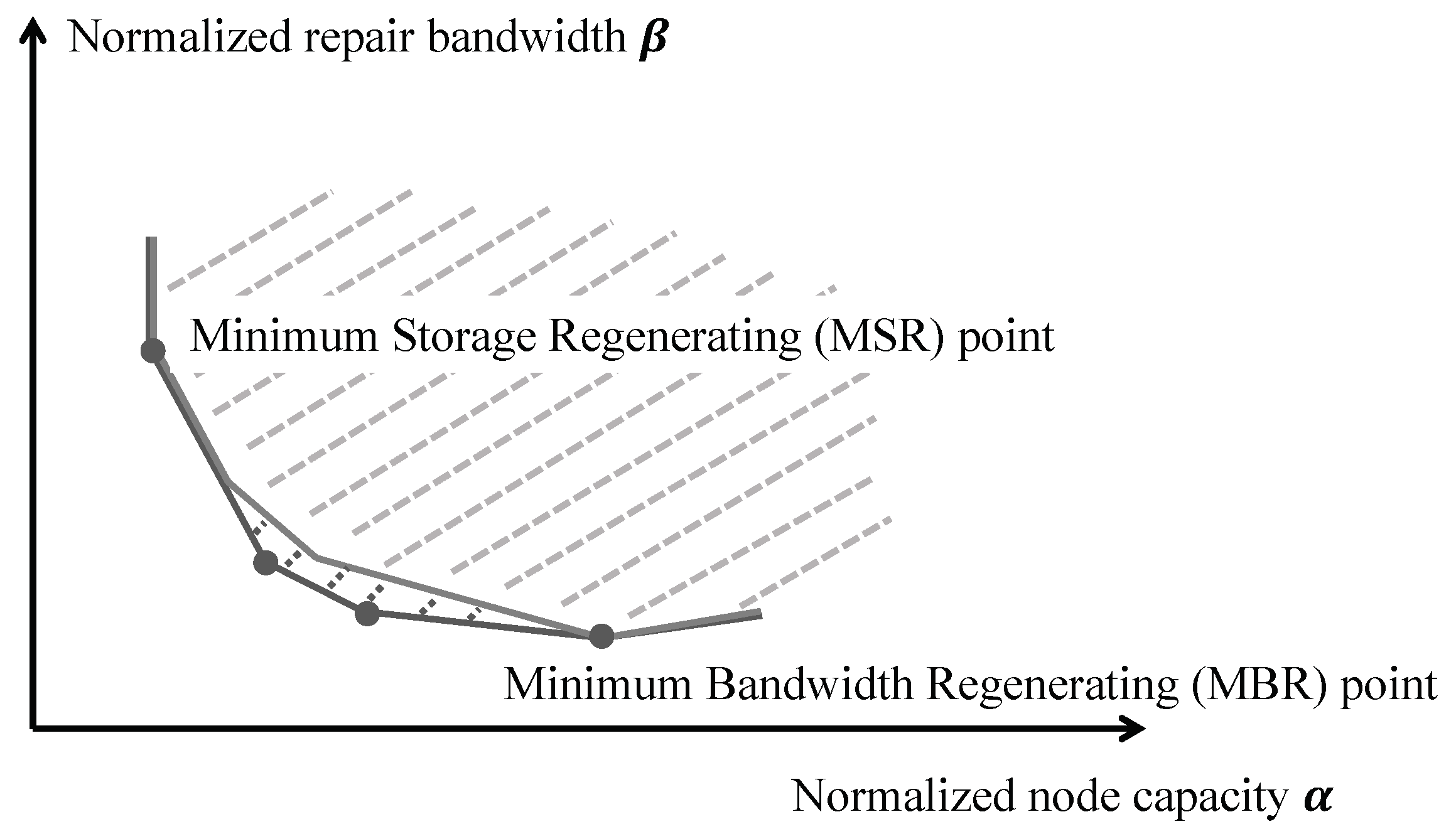
