

R Version of the Kedem–Katchalsky–Peusner Equations for Liquid Interface Potentials in a Membrane System


Abstract
1. Introduction
2. Materials and Methods
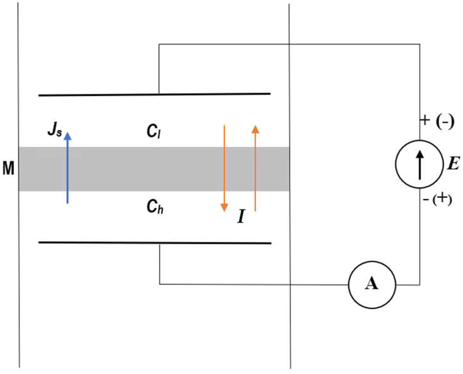
2.1. Membrane System
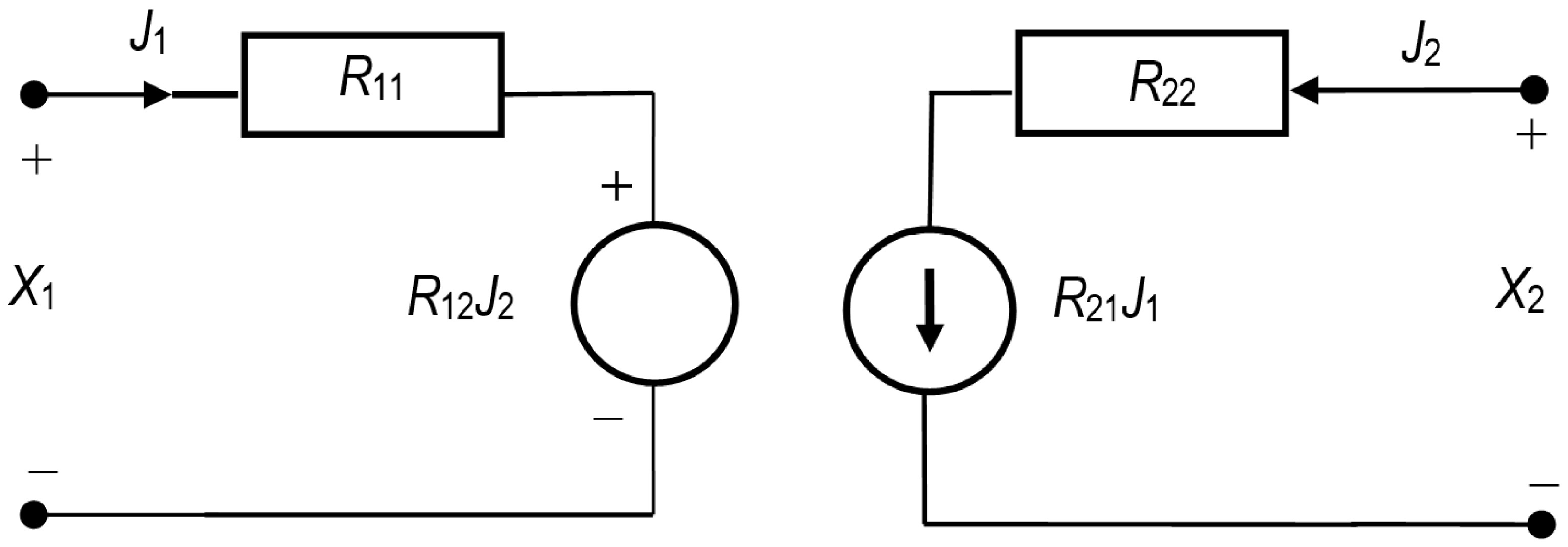
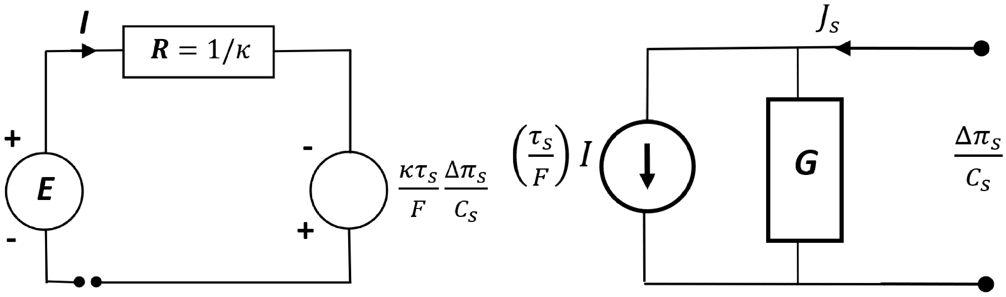
2.2. R Version of the Kedem–Katchalsky–Peusner Equations
2.3. Mathematical Model of Energy Conversion in the Membrane System
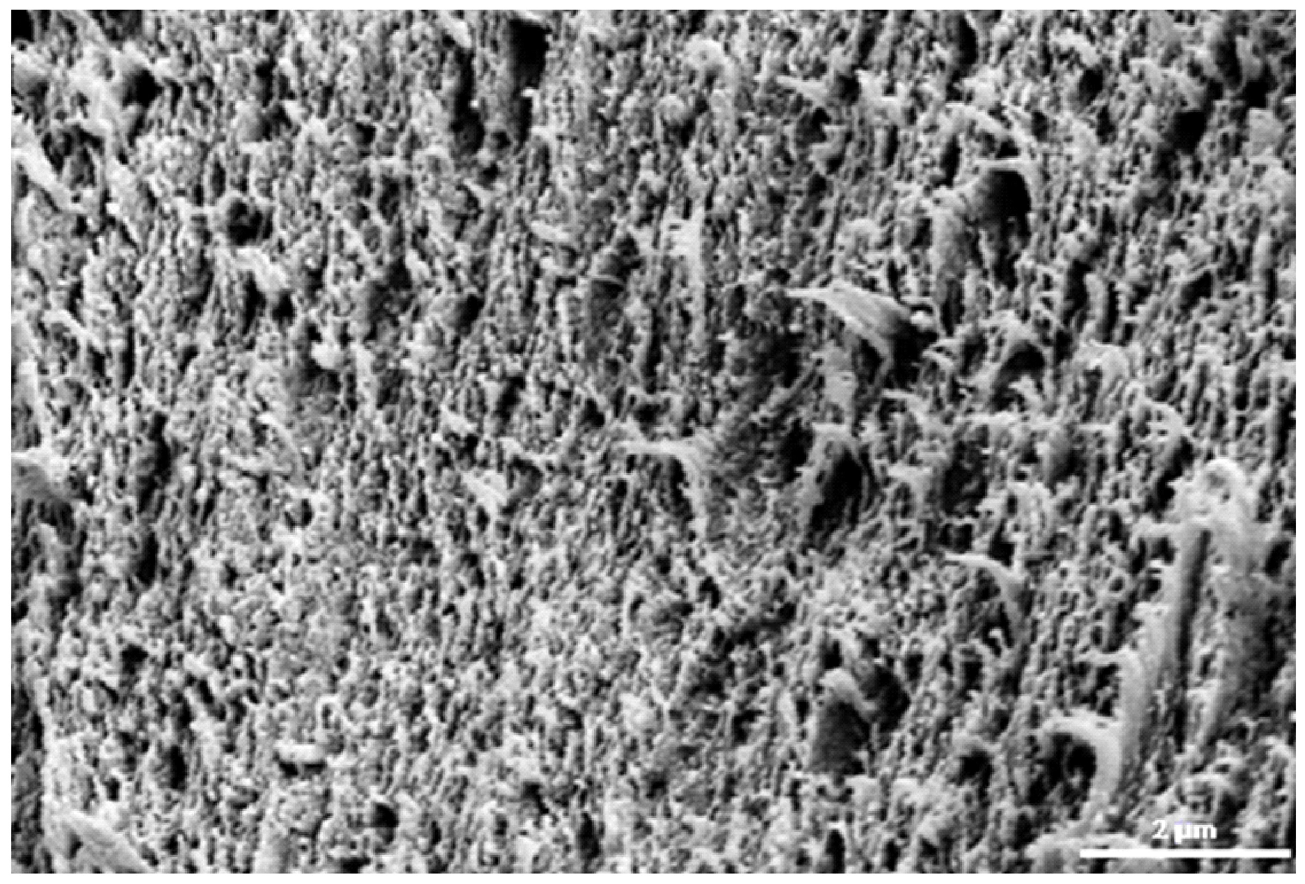
2.4. Biomembrane Characteristics
3. Results and Discussion
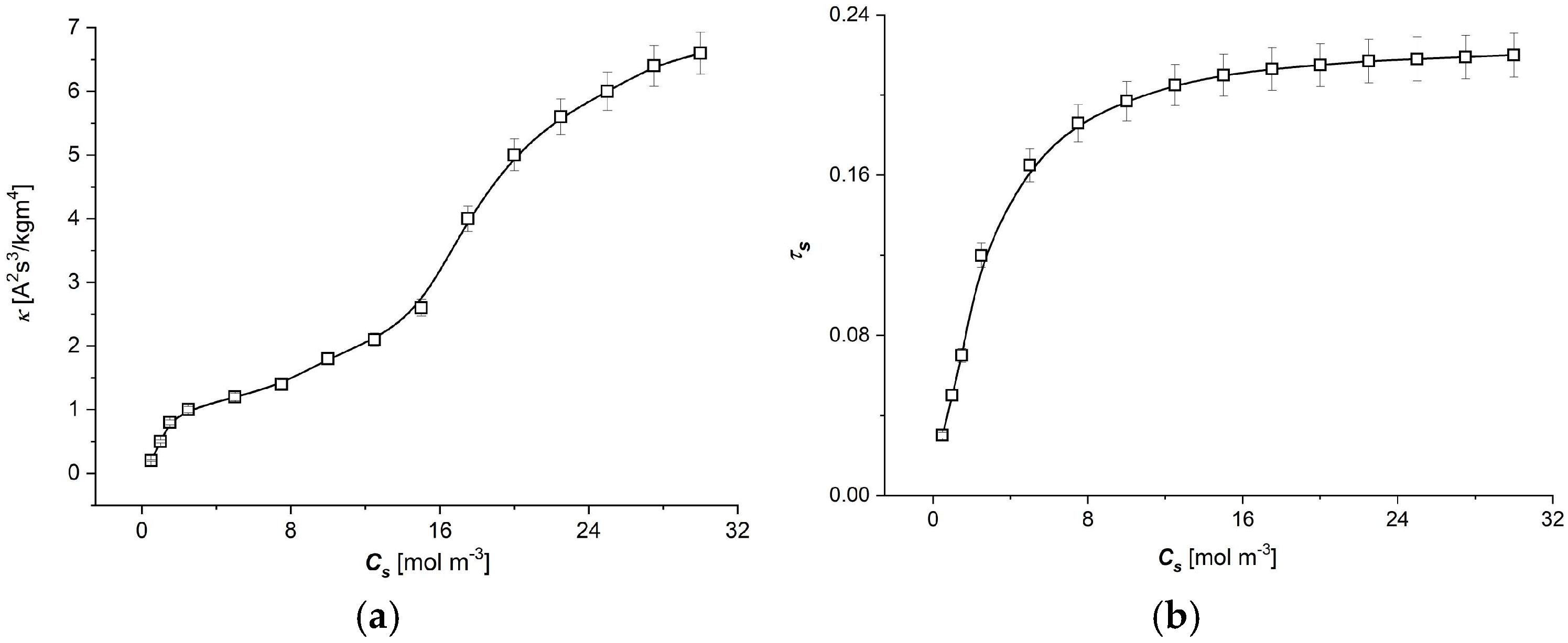
3.1. The Characteristic ) ( ∈ {1, 2})
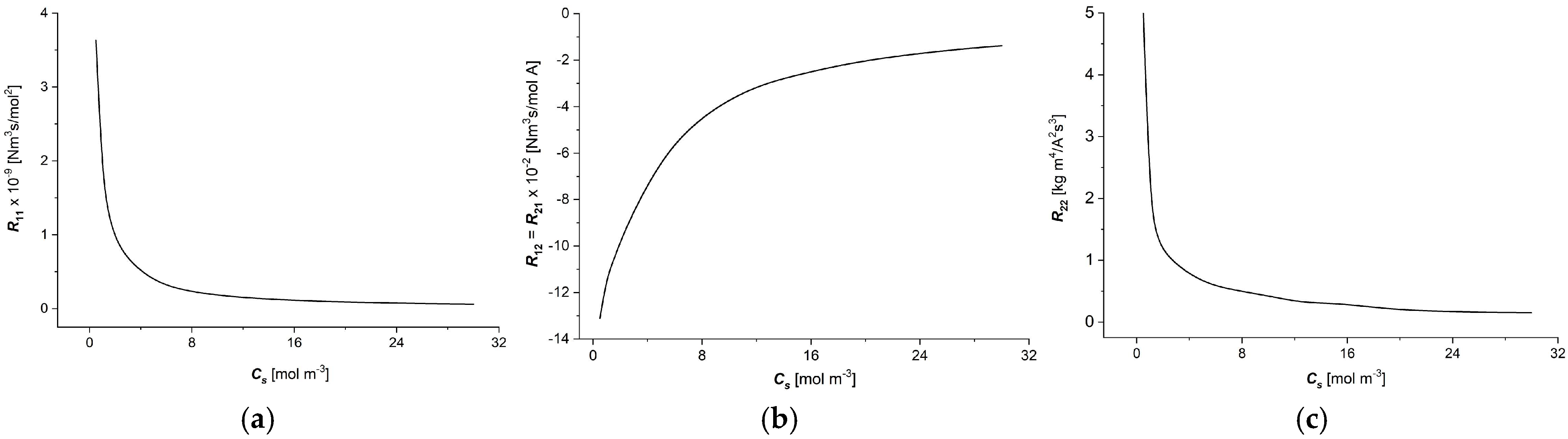
3.2. Characteristics , ( ∈ {1, 2, 3})
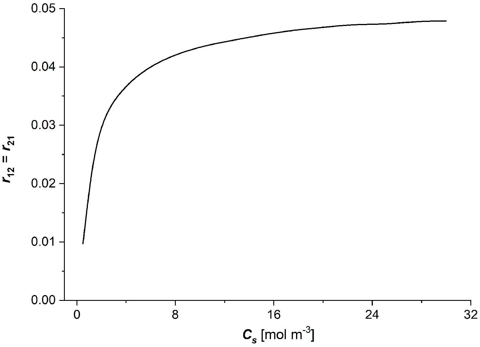
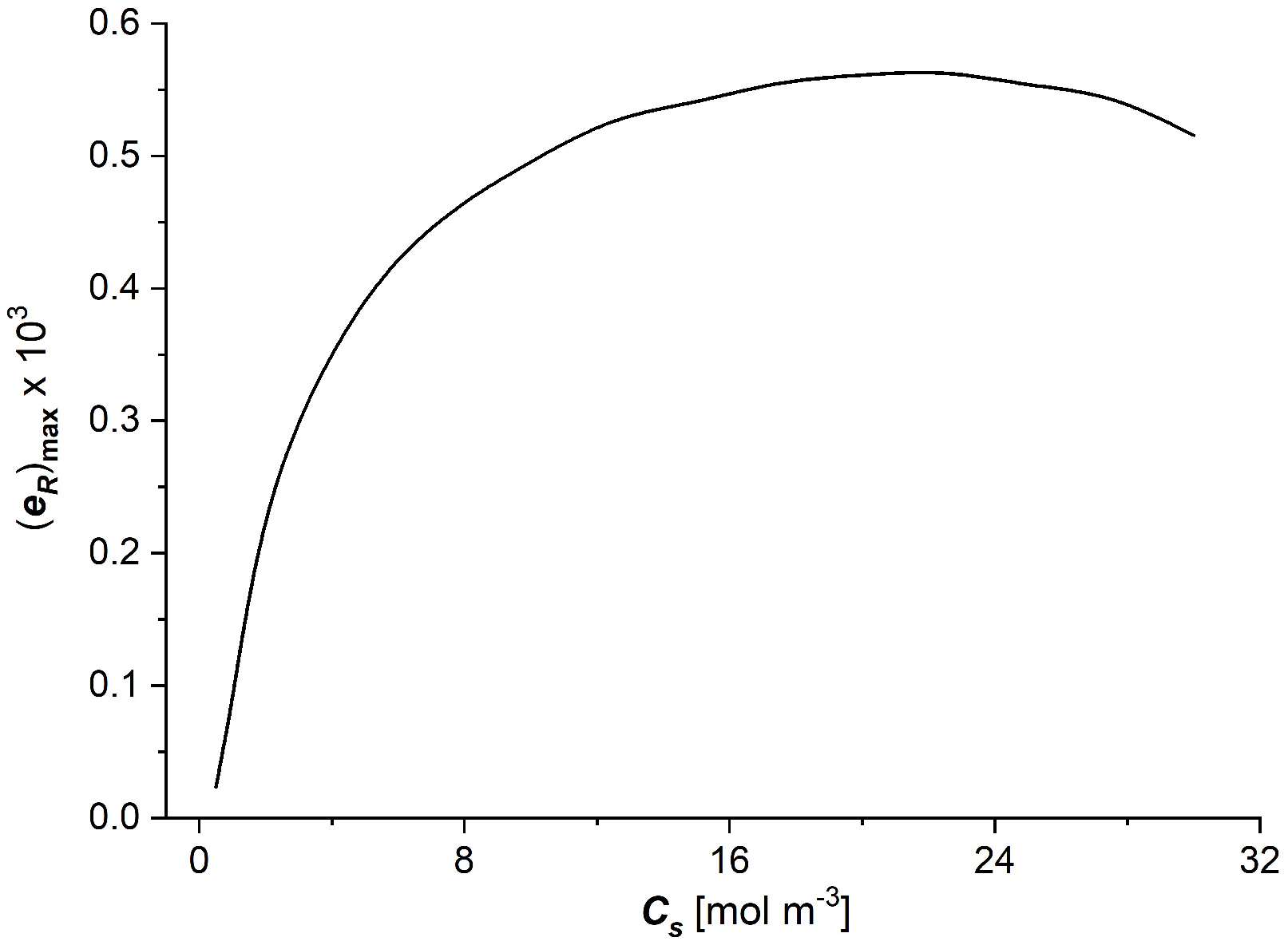
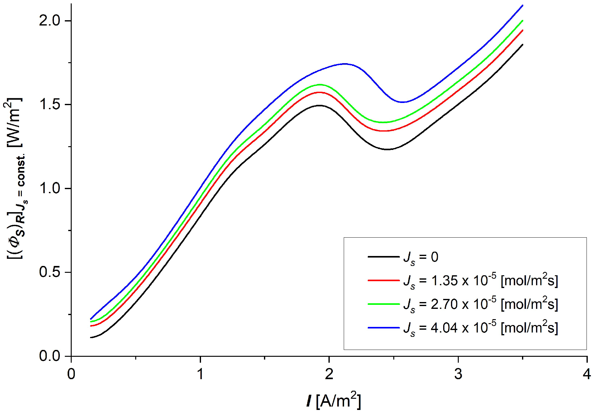
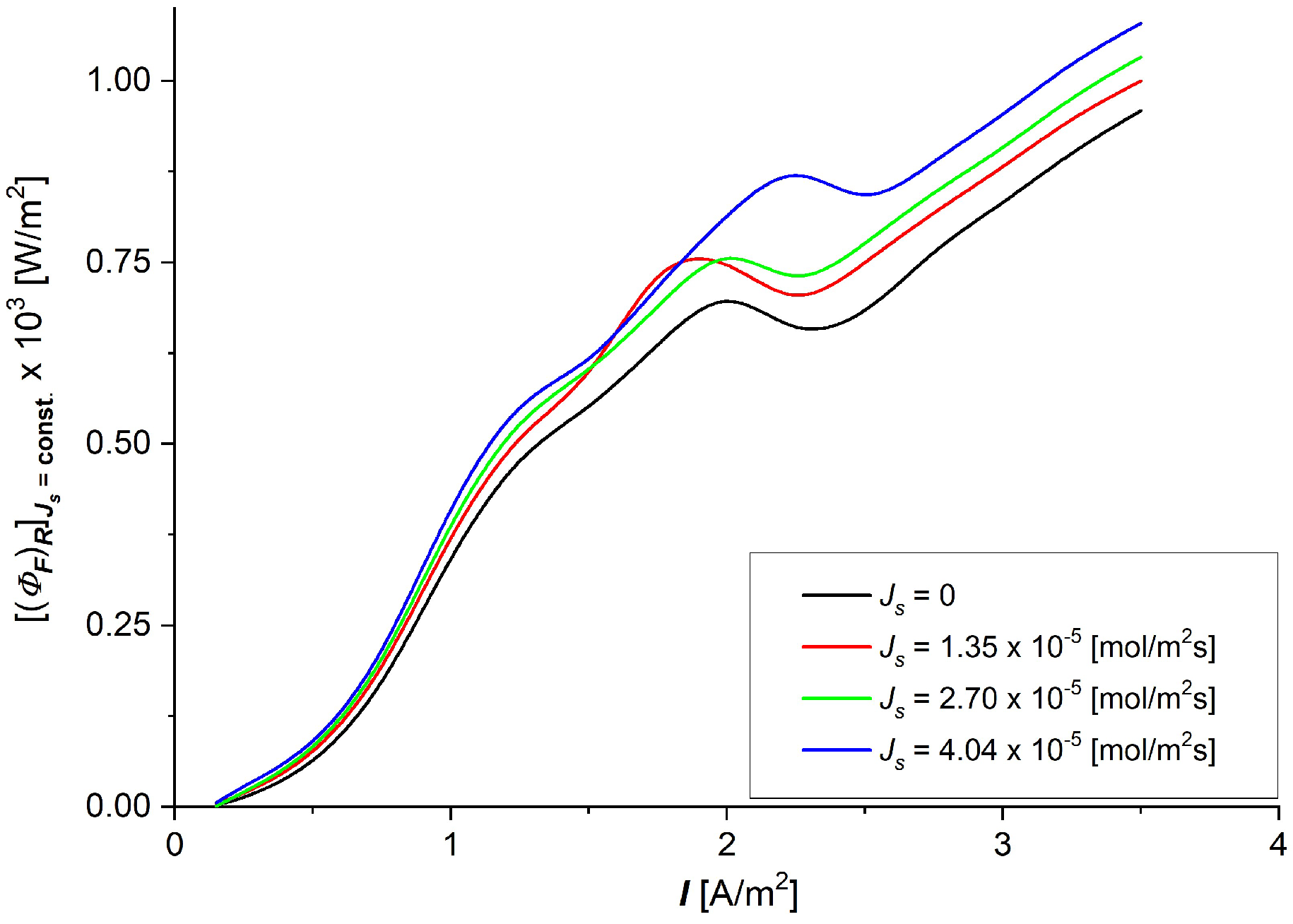
3.3. The Characteristics and
4. Discussion
5. Conclusions
- The moduli of resistant coefficients of the Ultra Flo Dialyser membrane decrease nonlinearly with the increasing NaCl concentration in the membrane, and the main changes in these coefficients are observed for low NaCl concentrations at less than 8 mol/m3.
- The coefficients of the degree of coupling of processes and energy conversion efficiency increase nonlinearly with the increasing NaCl concentration in the membrane; the main changes in these coefficients were also observed for low NaCl concentrations, less than 8 mol/m3. The value of the energy conversion efficiency coefficients for NaCl concentration in the membrane greater than 8 mol/m3 is greater than 0.5.
- The dissipated energy flux during membrane processes is much larger than the useful energy flux for these processes, so the internal energy of the flux is completely converted during membrane processes into the flux of dissipated energy.
Author Contributions
Funding
Institutional Review Board Statement
Data Availability Statement
Conflicts of Interest
List of Symbols and Abbreviations
| gas constant [J/molK] | |
| temperature [K] | |
| Faraday constant [C/mol] | |
| solute permeability coefficient [mol/Ns] | |
| transference number | |
| conductance coefficient | |
| osmotic pressure difference [Pa] | |
| solutions concentration difference [mol/m3] | |
| , | solutes concentrations [mol/m3] |
| average concentration of solutes [mol/m3] | |
| solute flux [mol/m2s] | |
| electric ionic current [A/m2] | |
| the Peusner’s resistant coefficients | |
| coupling coefficient of membrane processes | |
| ( | energy conversion efficiency coefficient |
| flux of S-energy [W/m2] | |
| flux of F-energy [W/m2] | |
| flux of U-energy [W/m2] | |
| K | distribution coefficient for salt between aqueous solution and membrane |
| volume of water in membrane | |
| ϑ | winding coefficient of channels in membrane |
| friction coefficient between i-th ion and water molecules | |
| friction coefficient between i-th ion and membrane | |
| friction coefficient in free solution | |
| PNT | Peusner’s network thermodynamics |
| NT | network thermodynamics |
| M | membrane |
| K-K-P equations | Kedem–Katchalsky–Peusner equations |
References
- Baker, R. Membrane Technology and Application; John Wiley & Sons: New York, NY, USA, 2012. [Google Scholar]
- Radu, E.R.; Voicu, S.I.; Thakur, V.K. Polymeric membranes for biomedical applications. Polymers 2023, 15, 619. [Google Scholar] [CrossRef]
- Dorotkiewicz-Jach, A.; Markowitz, P.; Rachuna, J.; Arabski, M.; Drulis-Kawa, Z. The impact of agarose immobilization on the activity of lytic Pseudomonas araginosa phages combined with chemicals. Appl. Microbiol. Biotechnol. 2023, 107, 897–913. [Google Scholar] [CrossRef] [PubMed]
- Zhang, Y.; Yu, L.; Zhang, X.-D.; Wang, Y.-H.; Yang, C.; Liu, X.; Wang, W.-P.; Zhang, Y.; Li, X.-T.; Li, G.; et al. A smart risk-responding polymer membrane for safer batteries. Sci. Adv. 2023, 9, eade5802. [Google Scholar] [CrossRef] [PubMed]
- Bolto, B.; Zhang, J.; Wu, X.; Xie, Z. A review on current development of membranes for oil removal from wastewaters. Membranes 2020, 10, 65. [Google Scholar] [CrossRef]
- Yahya, L.A.; Tobiszewski, M.; Kubica, P.; Koronkiewicz, S.; Vakh, C. Polymeric porous membranes as solid support and protective material in microextraction processes: A review. TrAC Trends Anal. Chem. 2024, 173, 117651. [Google Scholar] [CrossRef]
- Demirel, Y. Nonequilibrium Thermodynamics: Transport and Rate Processes in Physical, Chemical and Biological Systems, 2nd ed.; Elsevier: Amsterdam, The Netherlands; Heidelberg, Germany, 2007. [Google Scholar]
- Ślęzak, A.; Grzegorczyn, S.M. Network derivation of liquid junction potentials in single-membrane system. Membranes 2024, 14, 140. [Google Scholar] [CrossRef]
- Katchalsky, A.; Curran, P.F. Nonequilibrium Thermodynamics in Biophysics; Harvard University Press: Cambridge, UK, 1965. [Google Scholar]
- Paynter, H. Analysis and Design of Engineering Systems; MIT: Cambridge, UK, 1961. [Google Scholar]
- Meixner, J. Thermodynamics of electrical networks and Onsager-Casimir reciprocal relation. J. Math. Phys. 1963, 4, 154–159. [Google Scholar] [CrossRef]
- Peusner, L. The Principles of Network Thermodynamics and Biophysical Applications. Ph.D. Thesis, Harvard University, Cambridge, UK, 1970. [Google Scholar]
- Oster, G.F.; Perelson, A.; Katchalsky, A. Network Thermodynamics. Nature 1971, 234, 393–399. [Google Scholar] [CrossRef]
- Peusner, L. Hierarchies of irreversible energy conversion systems: A network thermodynamic approach. I. Linear steady state without storage. J. Theor. Biol. 1983, 102, 7–39. [Google Scholar] [CrossRef]
- Peusner, L. Hierarchies of irreversible energy conversion systems. II. Network derivation of linear transport equations. J. Theor. Biol. 1985, 115, 319–335. [Google Scholar] [CrossRef]
- Peusner, L. Studies in Network Thermodynamics; Elsevier: Amsterdam, The Netherlands; New York, NY, USA, 1986. [Google Scholar]
- Batko, K.M.; Slezak-Prochazka, I.; Grzegorczyn, S.; Ślęzak, A. Membrane transport in concentration polarization conditions: Network thermodynamics model equations. J. Porous Media 2014, 17, 573–586. [Google Scholar] [CrossRef]
- Onsager, L. Reciprocal Relations in Irreversible Processes. I. Phys. Rev. 1931, 37, 405–426. [Google Scholar] [CrossRef]
- Peusner, L. Global reaction: Diffusion coupling and reciprocity in linear asymmetric kinetic networks. J. Chem. Phys. 1982, 77, 5500–5507. [Google Scholar] [CrossRef]
- Mikulecky, D.C. When is a mechanism not a mechanism? The network thermodynamic approach to complex systems. Math. Comput. Model. 1988, 11, 464–468. [Google Scholar] [CrossRef]
- Mikulecky, D.C. Network thermodynamics and complexity: A transition to relational systems theory. Comput. Chem. 2001, 25, 369–391. [Google Scholar] [CrossRef]
- Gawthrop, P.J.; Pan, M. Network thermodynamics of biological systems: A bond graph approach. Math. Biosci. 2022, 352, 108899. [Google Scholar] [CrossRef]
- Avanzini, F.; Freitas, N.; Esposito, M. Circuit theory for chemical reaction networks. Phys. Rev. X 2023, 13, 021041. [Google Scholar] [CrossRef]
- Zitzmann, C.; Dächert, C.; Schmid, B.; van der Schaar, H.; van Hemert, M.; Perelson, A.S.; van Kuppeveld, F.J.M.; Bartenschlager, R.; Binder, M.; Kaderali, L. Mathematical modeling of plus-strand RNA virus replication to identify broad-spectrum antiviral treatment strategies. PLoS Comput. Biol. 2023, 19, e1010423. [Google Scholar] [CrossRef]
- Mogilner, A.; Oster, G. Cell motility driven by actin polymerization. Biophys. J. 1996, 71, 3030–3045. [Google Scholar] [CrossRef]
- Oster, G. Clocks and patterns in Myxobacteria: A remembrance of Art Winfree. J. Theor. Biol. 2004, 230, 451–458. [Google Scholar] [CrossRef]
- Lachenbruch, C.A.; Diller, K.R. A network thermodynamic model of kidney perfusion. IFAC Proc. Vol. 1994, 27, 289–290. [Google Scholar] [CrossRef]
- Horno, J.; González-Fernández, C.F.; Hayas, A.; González-Caballero, F. Simulation of concentration polarization in electrokinetic processes by network thermodynamic methods. Biophys. J. 1989, 55, 527–535. [Google Scholar] [CrossRef] [PubMed]
- Mamedov, M.M. Phenomenological derivation of the Onsager reciprocal relations. Tech. Phys. Lett. 2003, 29, 676–678. [Google Scholar] [CrossRef]
- Filippov, A.N. A Cell model of an ion-exchange membrane. capillary-osmosis and reverse-osmosis coefficients. Colloid J. 2022, 84, 332–343. [Google Scholar] [CrossRef]
- Kedem, O.; Caplan, S.R. Degree of coupling and its relation to efficiency of energy conversion. Trans. Faraday Soc. 1965, 61, 1897–1911. [Google Scholar] [CrossRef]
- Caplan, S.R. Nonequilibrium thermodynamics and its application to bioenergetics. Curr. Top. Bioenerg. 1971, 4, 1–79. [Google Scholar] [CrossRef]
- Twardowski, Z.J. History of hemodialyzers’ designs. Hemodial. Int. 2008, 12, 173–210. [Google Scholar] [CrossRef]
- Grzegorczyn, S. Effects of Concentration Polarization of Flat Bacterial Cellulose Membranes; Silesian Medical Academy Press: Katowice, Poland, 2006. (In Polish) [Google Scholar]
Disclaimer/Publisher’s Note: The statements, opinions and data contained in all publications are solely those of the individual author(s) and contributor(s) and not of MDPI and/or the editor(s). MDPI and/or the editor(s) disclaim responsibility for any injury to people or property resulting from any ideas, methods, instructions or products referred to in the content. |
© 2025 by the authors. Licensee MDPI, Basel, Switzerland. This article is an open access article distributed under the terms and conditions of the Creative Commons Attribution (CC BY) license (https://creativecommons.org/licenses/by/4.0/).
Share and Cite
Ślęzak, A.; Grzegorczyn, S.M. R Version of the Kedem–Katchalsky–Peusner Equations for Liquid Interface Potentials in a Membrane System. Entropy 2025, 27, 169. https://doi.org/10.3390/e27020169
Ślęzak A, Grzegorczyn SM. R Version of the Kedem–Katchalsky–Peusner Equations for Liquid Interface Potentials in a Membrane System. Entropy. 2025; 27(2):169. https://doi.org/10.3390/e27020169
Chicago/Turabian StyleŚlęzak, Andrzej, and Sławomir M. Grzegorczyn. 2025. "R Version of the Kedem–Katchalsky–Peusner Equations for Liquid Interface Potentials in a Membrane System" Entropy 27, no. 2: 169. https://doi.org/10.3390/e27020169
APA StyleŚlęzak, A., & Grzegorczyn, S. M. (2025). R Version of the Kedem–Katchalsky–Peusner Equations for Liquid Interface Potentials in a Membrane System. Entropy, 27(2), 169. https://doi.org/10.3390/e27020169