Abstract
A kinetic exchange model is developed to investigate wealth distribution in a market. The model incorporates a value function that captures the agents’ psychological traits, governing their wealth allocation based on behavioral responses to perceived potential losses and returns. To account for the impact of transaction frequency on wealth dynamics, a non-Maxwellian collision kernel is introduced. Applying quasi-invariant limits and Boltzmann-type equations, a Fokker–Planck equation is derived. We obtain an entropy explicit stationary solution that exhibits exponential convergence to a lognormal wealth distribution. Numerical experiments support the theoretical insights and highlight the model’s significance in understanding wealth distribution.
1. Introduction
The investigation of wealth distribution has been carried out through the application of kinetic and statistical models, which provide a robust theoretical framework for analyzing complex socioeconomic phenomena. These models, fundamentally grounded in probability theory and statistical mechanics, have proven to be useful in elucidating the underlying mechanisms of wealth distribution [1], opinion formation [2], and knowledge accumulation [3]. In particular, by simulating interactions between individual agents, researchers have been able to replicate and analyze the emergence of power-law tails and other complex features in wealth distribution [4].
Bouchaud and Mezard [5] introduced the collision operator (Fokker–Planck operator) to describe the process of wealth exchange. Chakraborti and Chatterjee [1] developed wealth exchange models by using the theory of rarefied gas dynamics to study wealth distribution problems. Cordier et al. [4] established a rule for wealth exchange based on the binary interaction followed by gas molecule collisions, integrating economic market behavior into the model. They applied a scale transformation to derive the Fokker–Planck operator. The results in [4] indicate that the density function of the wealth distribution satisfies a Boltzmann equation, and the steady-state solution of its Fokker–Planck equation is an inverse Gamma function, implying the presence of a Pareto tail in the steady-state wealth distribution. Bertotti [6] considered a model of the taxation and redistribution process in a closed society. Toscani [2] presented a kinetic model of continuous opinion formation, accounting for both opinion exchange between agents and information diffusion. Düring et al. [7] used a Boltzmann-type control model to analyze how leaders adjust their strategies based on an objective functional to achieve opinion consensus, leveraging an instantaneous binary control formulation that integrates cost minimization into their interactions. From the Boltzmann-type equation, the Fokker–Planck equation is derived, which gives explicit stationary solutions. Pareschi and Toscani [3] proposed a nonlinear Boltzmann-type kinetic equation, incorporating trade parameters such as risk awareness and saving propensity decided by the individual knowledge of the agent. This model aims to explore how variations in knowledge levels influence the evolution of wealth distribution among agents. Numerical simulations illustrate that high levels of knowledge can give rise to a wealthy class and exacerbate wealth inequality.
Recent developments have emphasized the incorporation of behavioral economic principles, particularly the integration of individual characteristic variables (such as beliefs and reliabilities), which are embedded in the agents’ strategies in microdynamic wealth exchange models, thereby making the model more realistic. Specifically, Brugna and Toscani [8] explored a nonlinear Boltzmann-type kinetic equation that incorporates the impact of individual conviction on opinion formation among agents, modifying binary exchanges by allowing the compromise and diffusion terms to depend on conviction levels. Numerical simulations reveal that conviction can break symmetry and generate opinion clusters. Toscani et al. [9] investigated wealth distribution by employing a value function to model the psychological behavior of agents engaged in strategic interactions, indicating that the wealth distribution of the agents adheres to a lognormal distribution. In the investigation of wealth distribution within financial markets, Hu and Lai [10] analyzed how variations in knowledge levels affect wealth allocation in the stock market. It was found in [10] that the psychological traits of agents could be effectively described using a value function that incorporates both the present price of stock and its essential value. Zhong et al. [11] considered a value function relating to agents’ risk perception behavior, which characterizes the proportion of wealth allocation between risky and riskless assets. By integrating this value function into the interaction rules between stocks and bonds, the authors in [11] examined the micro-level variations in investment strategies influenced by price and risk factors, concluding that the wealth invested in stocks also converges to a lognormal distribution.
In addition, in the context of wealth distribution models based on Boltzmann dynamics, the traditional approach utilizes a Maxwellian collision kernel, which presumes a constant interaction frequency among agents engaged in market activities. This reflects the assumption that agents interact uniformly, regardless of their wealth, implying a sort of ‘egalitarian’ trading behavior in the system. In contrast, non-Maxwellian collision kernels (such as power and linear collision kernels) allow for more realistic interaction patterns that take the agents’ wealth into account.
Furioli et al. [12] proposed a non-Maxwellian collision kernel incorporated into the Boltzmann collision integral operator, implying that the interaction frequency between agents varies, rather than remaining constant. Additionally, an update rule for the evolution of agent wealth is proposed in [12], where a Fokker–Planck equation is derived from the Boltzmann equation and the corresponding wealth distribution is analyzed.
Recently, scholars have highlighted the effectiveness of kinetic models in capturing the nuances of asset trading and wealth evolution. Building upon these foundations, particularly the work in [11], in this paper, we focus on a financial market characterized by the presence of both a risky asset (such as a stock) and a riskless asset (like a bond). We develop a kinetic exchange model to explore how wealth is distributed among agents engaged in speculative trading and wealth exchanges. Our contributions are central to three points, as follows.
(i) The value function used to describe the asset allocation of agent in Zhong et al. [11] is
where is a constant, and and are the current price and intrinsic price of the stock, respectively. We choose a different value function to illustrate the feature of binary interaction dynamics based on the evolution that agents shift wealth between two assets, which reads as
where is a key parameter in modeling the behavior of agents, capturing the influence of psychological characteristics during trading. This value function reflects agents’ behavioral responses to potential returns and losses, depending not only on the intrinsic price and current price of the risky asset but also on the parameter . In the value function , parameter is explained as a parameter of psychological traits that depict the agents’ strategies, which are affected by psychological tendencies during trading. Specifically, the introduction of causes the value function to approach the reference point more gradually when the current stock price exceeds its intrinsic price, as seen in Figure 1. This setting suggests that agents slowly adjust their portfolios, showing reluctance to reduce stock holdings in response to elevated prices of risky assets, which reflects their psychological traits in profit maximization under such market conditions. This behavior aligns with the trading patterns commonly observed in financial markets.
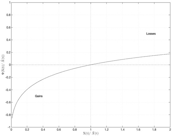
Figure 1.
The illustration of value function .
(ii) Inspired by the work in [12], we apply a non-Maxwellian collision kernel relating with the frequency of wealth exchange to consider the effect of the transaction frequency among agents. By contrast with the work in Zhong et al. [11] where the constant collision kernel was used, we analyze the impact of agents’ transaction frequency on the evolution of wealth distribution.
(iii) The stationary solution we obtained is different from those in Zhong et al. [11]. Our stationary solution is related with parameter of transaction frequency and parameter of psychological traits, which was not considered in [11].
To validate our theoretical results, we conduct numerical experiments that illustrate the dynamics of wealth distribution under various scenarios. These experiments not only confirm the robustness of our model but also provide deep insights into the factors that affect the long-term behavior of wealth distribution in financial markets.
This paper is structured as follows: Section 2 describes the construction of the kinetic exchange model and the incorporation of the value function. Section 3 discusses the main properties of the kinetic equation. Section 4 presents the derivation of the Fokker–Planck equation and the existence of a stationary solution. Section 5 offers a detailed analysis of the numerical experiments, while Section 6 concludes with a summary of our results.
2. A Kinetic Description of Wealth Distribution
In essence, the kinetic model of wealth exchange in our paper is inspired by the model in Zhong et al. [11]. We consider that agents in the market equipped with a risky asset (stock) and a risk-free asset (bond) as their wealth, aiming to describe the evolution of wealth distribution. We assume that the agents are homogeneous, with non-negative wealth, and that the allocation of such assets can be adjusted at any point in time. Thus, we depict the dynamics of wealth distribution among agents via the interplay of the two kinds of assets.
Considering the microscopic interplay of the risky and risk-free assets (stocks and bonds), we apply to denote each agent’s wealth invested in stocks, and use to denote the rest part invested in bonds. Furthermore, companying agents trading with others in the market, an agent’s wealth before interaction is adjusted to the post-interaction . Then, we depict the interaction rule as follows
where the non-negative coefficients and are variables related to the stock’s price.
Generally, portfolio management involves making choices. As agents continuously adjust their investment strategies based on predictions of future market conditions, agents determine the proportion of their investments in both risky and risk-free assets at each stage of the process. Consequently, the price dynamics of the risky asset are affected by the portfolio decisions, which are made by agents. We assume that the profit rate of the risk-free asset is a fixed interest rate , and the profit rate of the risky asset is described by
where is the stock price at time t, is the dividend, and denotes the time derivative of . We define the current price of the stock by using the formulation in [11], which reads as
where represents the average investment propensity of agents, which satisfies , and parameter indicates the rate of price evolution. Equation (2) shows that the current stock price is related to the average investment propensity of agents, which is based on the idea in [13].
In fact, comparing the return from the investment of bond, agents strategically adjust their stock holdings in the next step to maximize their profits. We define the stock’s excess profit rate which is denoted by as follows
where represents the predictable stock price. Equation (3) implies the potential gain or loss comparing with investing in bonds.
Note that, when the profit rate of the investment in risky assets is equal to the profit rate of risk-free assets, the stock’s intrinsic price, which is denoted by , satisfies
We infer from Equation (4) that the intrinsic price of the stock relating to the stock’s predictable price influences the excess profits of the agent, and consequently affects the agent’s investment decision.
According to the prospect theory in [14,15], agents formulate and carry out their investment strategy to get excess profit by identifying the gap between the stock’s current price and intrinsic price. To be specific, when
we have
The fixed interest rate of the bond is below the profit rate of the stock, leading to a positive excess profit rate that compels agents to shift their wealth from the bond to the other asset. Conversely, when
we have
Owing to , the investment in the bond has relatively higher yields, and so agents would like to make a reduction gradually on their investment in stocks.
In order to investigate the exchanges of wealth, we introduce a value function which satisfies
and
In Equation (5), z represents a positive variable, and denotes random variables that capture market fluctuations, with zero mean and variance , while is a constant that quantifies the proportion of wealth transferred between assets. According to [4], it can be explained as a transaction coefficient.
By substituting into Equation (1), we derive the following binary interaction model, which characterizes the wealth distribution’s microscopic dynamics between the investments of risky and riskless assets, which reads
We choose the value function as
where represents an appropriate parameter to describe the behavior of the agent affected by psychological traits. The exponent is a constant that controls how strongly the value function responds to the ratio between the current price and the intrinsic price of risky assets. Actually, we notice that . Then, we find that the value function is bounded, which satisfies
Figure 1 illustrates that the value function represents the deviation from a reference point where . Specifically, for , the value function is positive, indicating risk-seeking behavior in response to losses. In contrast, for , the function becomes negative and convex, reflecting risk aversion in the presence of gains.
Compared to the work in Zhong et al. [11], the primary distinction is observed on the right side of the reference point, where . As shown in Figure 1, the curve of is smoother than the left side. In this regard, the value function approaches the reference point relatively slower when the current price of the stock exceeds the intrinsic price. This setup implies that agents gradually adjust their portfolios and sell stocks with hesitation in response to rising prices of risky assets, reflecting their psychological tendencies in profit maximization during such market conditions. This behavior is consistent with trading patterns frequently observed in financial markets.
3. The Kinetic Description of Wealth
In this part, we consider a Boltzmann dynamic according to the above binary interaction to derive a kinetic equation to study the evolution of wealth distribution. We introduce a density function , where at time . The specific meaning of the density h is as follows. Given the system of traders, and given an interval or a more complex sub-domain , the integral
represents the number of traders who are characterized by an amount of wealth at time . It is assumed that the density function is normalized to one; that is, for all
Additionally, we suppose that the total amount of the stock owned by an agent, denoted by n, is fixed. Then, we use to denote the current value of wealth aligned with the stock, while the expected value of wealth attributable to the stock under the predictability is represented by . Thus, we obtain
In rule (6), the value function quantifies the variations relative to the reference point where . The value function is positive above the reference point and negative below the reference point .
Based on the interaction rule (6), the density function, which is denoted by , satisfies the weak form of the Boltzmann-type equation. Specifically, for any smooth test function defined on , the density function acts as the weak solution of the equation
where symbol denotes the mathematical expectation, and is the collision kernel related to the transaction frequency of agents with constant and the parameter of transaction frequency , where .
Note that Equation (7) is derived from the kinetic equation as originally formulated in [16], where the collision kernel in the originated equation is a constant term. However, in our work, we introduce a non-Maxwellian collision kernel related to the frequency of wealth exchange in risky assets to account for the effect of transaction frequency among agents. Specifically, the introduction of transaction frequency parameter is intended to depict the interaction frequency of agents in the kinetic equation. In this context, the non-Maxwellian collision kernel we introduced is the power collision kernel (expressed as , where is the parameter of transaction frequency, is a constant, and v represents the wealth of the agent invested in risky assets), which indicates that agents who do not invest in risky assets are not involved in trading. It characterizes the frequency of stock transactions executed by the agent at each trading point in kinetic Equation (7). By contrast with the constant collision kernel in Zhong et al. [11], this is our innovation.
Remark 1.
In particular, the power collision kernel introduces a wealth-dependent interaction frequency, implying that the likelihood of interaction is no longer constant but rather varies based on the wealth of the agents. This models real-world phenomena where wealthier individuals may engage more frequently in trade or speculative activities, or where the willingness to trade might be influenced by wealth disparities between agents. This feature often observed in real-world economies but not captured by Maxwellian kernels.
Remark 2.
Compared to the power collision kernel, the linear collision kernel introduces a more direct relationship between agents’ wealth investment and their trading behavior. This type of kernel implies that the frequency of interaction between agents is a linear function of their wealth, which is different from the assumption of independent interactions in the general framework. In this case, wealthy agents might engage in trade at a rate proportional to their wealth, leading to differential impacts on wealth distribution. The interaction dynamics can generate varying levels of inequality based on how agents invest and interact, and the introduction of a bilinear kinetic model enhances the system’s ability to account for disparities in wealth investment across groups.
Remark 3.
While earlier kinetic models often assume random or uniform interactions (such as in the mean-field models), the non-Maxwellian kernel allow the kinetic model to capture more heterogeneity by varying the interaction frequency based on wealth. This is closer to agent-based models in economics, where agents have different wealth, psychological traits, and risk profiles, leading to more complex and often heterogeneous market dynamics. The approach of introducing a non-Maxwellian kernel also aligns with behavioral economics, which considers psychological factors, risk aversion, and other human behavioral aspects that affect economic decision-making. This incorporation of agents’ psychological traits into the wealth evolution process creates a more realistic representation of market behavior, as agents’ interactions are not purely determined by objective wealth maximization but also by subjective preferences, social influences, and expectations.
To be more precise, investigating the temporal behavior of the wealth distribution is inherently tricky due to the nonlinearity of the interaction described in the interaction rule (6). Therefrom, we analyze the fundamental characteristics of the kinetic equation.
Thanks to the entropy weak form of the Boltzmann-type equation, we can leave out the time dependence in this distribution function. Setting , we obtain the conservation of wealth in the system, meaning that Equation (7) is conserved. Namely,
where .
Now, taking in (7), we have that the evolution of average value of wealth satisfies
where
It follows from (8) that is a positive constant. Taking yields
We assume that the wealth v and w have the same density function h, which is given by
Utilizing the interaction rule (6), we obtain
Since , we have
Substituting (10) into (9) gives rise to
Although (11) has no explicit solution, we consider the value function and let
We have
Since is positive constant, and
utilizing inequality (12) yields
which derives
Then, we have
implying that the second moment remains bounded.
4. Fokker–Planck Modeling
In fact, solving Equation (11) poses certain difficulties. Under this circumstance, numerical simulation is a general way to discuss the problem. In order to analyze the solution, we use the asymptotic limits of the Boltzmann-type equation to derive the Fokker–Planck equation. The core idea is to introduce an appropriate scaling rule to derive the Fokker–Planck equation and consequently obtain the steady-state solution.
We introduce a very small variable , where . Let
Following the idea in [11], we set as
For smooth functions with supported set in , the corresponding distribution of wealth is denoted by at time . When , we have
Back to the properties of kinetic equation we discussed, we will derive the Fokker–Planck equation. We have
Using the second-order Taylor expansion of smooth function around v, we have
where . Thus, we obtain
where is the residual term, given by
Thus, we obtain the rescale equation which reads
in which satisfies
As , the reminder term satisfies
Therefore, we have the following equation as the residual term approaches zero, which is given by
Letting , and assuming that both and are sufficiently small, we derive the weak form
Using (13) yields
Then, we obtain the equation
Assuming that the boundary term resulting from the integral tends to zero as it approaches infinity, we consider that the boundary value of the density function is zero and obtain
and
From Equations (14) and (15), we derive the Fokker–Planck equation as follows
In Equation (16), the form of the quasi-invariant limit depicts the evolution of wealth distribution.
The Steady State Distribution of the Wealth
Rewriting Equation (16), we have
The Fokker–Planck Equation (17) depicts the behavior of the scaled density function for wealth v, where . As time approaches infinity, we have
From Equation (18), we investigate the steady state of Equation (17). The stationary solution of Equation (17) satisfies
which, in turn, has the stationary solution given by
Letting , we obtain the explicit steady-state distribution
where , and is the essential wealth of the agent based on the intrinsic price of the stock. In particular, constant in Equation (19) depends on the average wealth m, the parameter of transaction frequency , and related to and , satisfying
5. Numerical Simulations
This section presents an analysis of the steady-state profiles obtained from numerical simulations of the stationary wealth distribution. Basing on various key parameters, we observe how these profiles reflect the asymptotic behaviors of the steady-state solution to Equation (17), which is shown in Figure 2, Figure 3 and Figure 4.

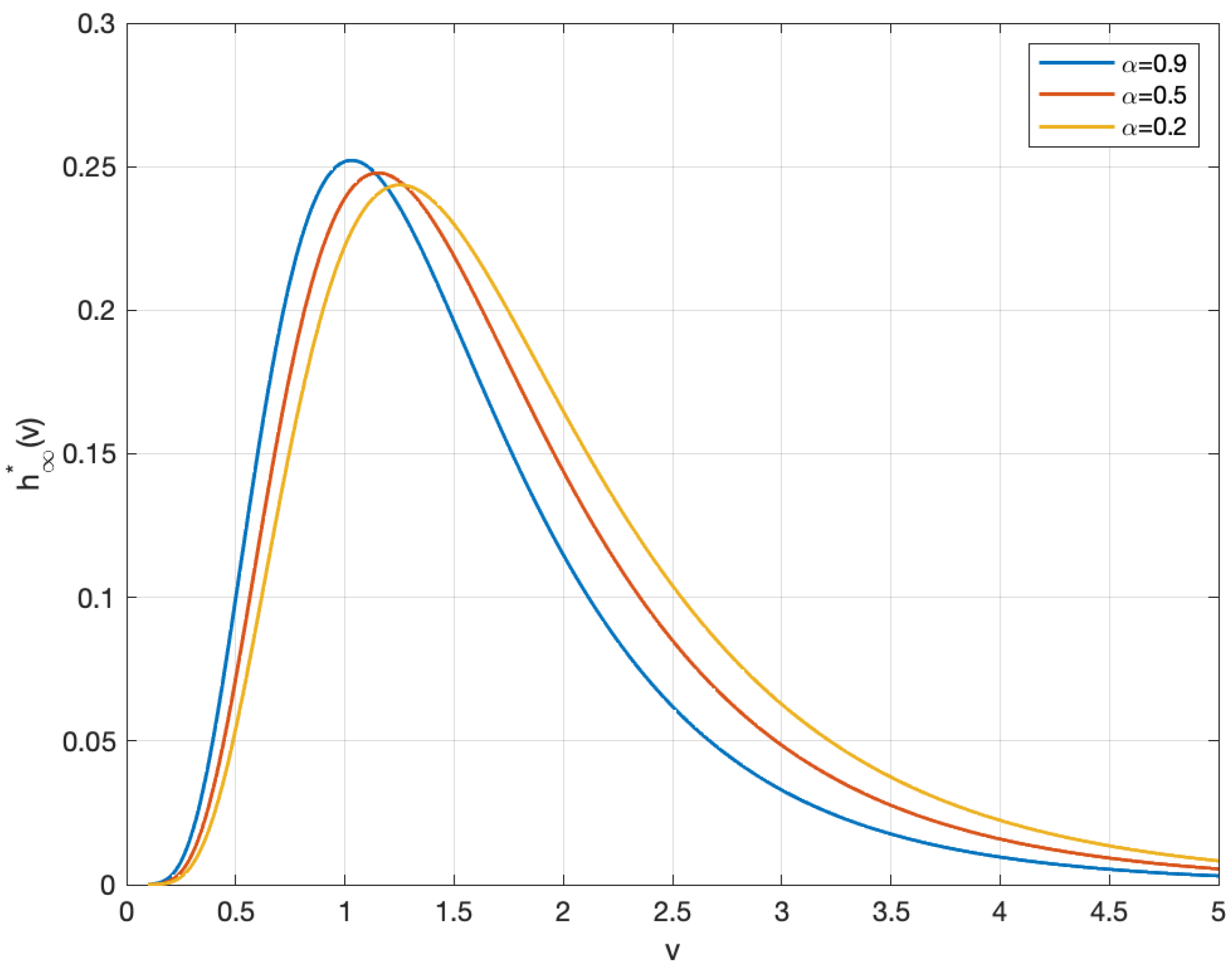
Figure 2.
The stationary profiles of wealth distribution for ; (blue line); (red line); (yellow line).
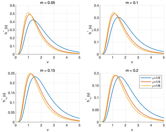
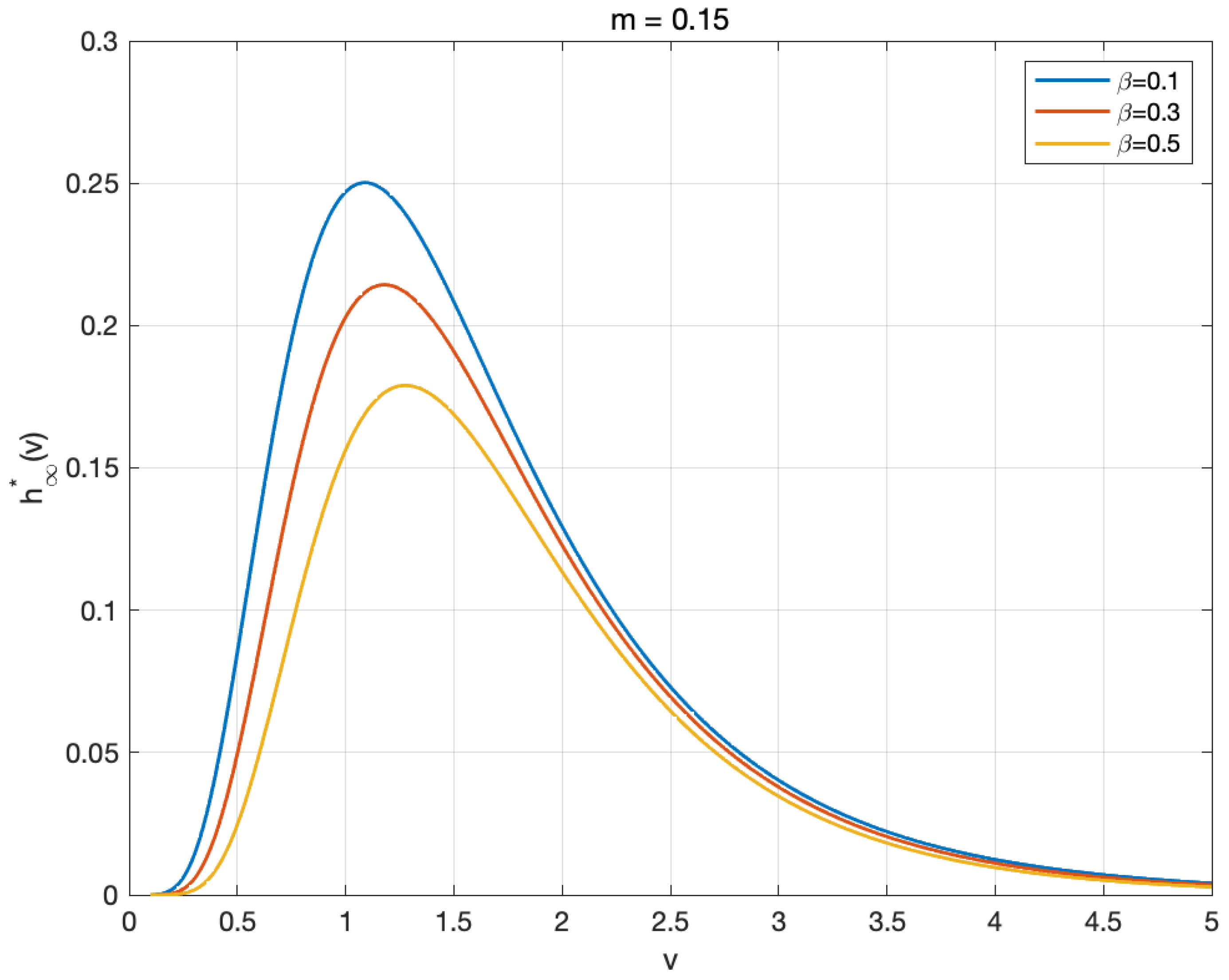
Figure 3.
The stationary profiles for (blue line), (red line), and (yellow line) with different values of m.
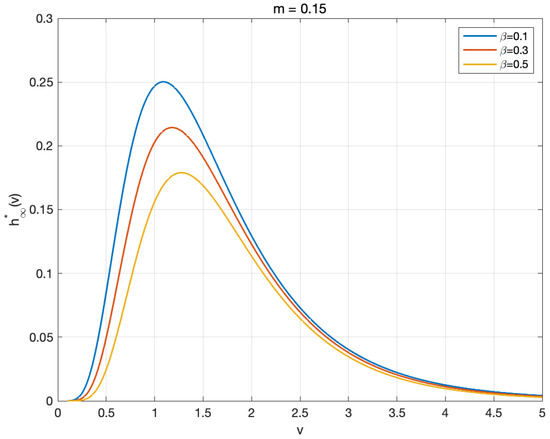
Figure 4.
Profiles of the stationary solution for (blue line), (red line), and (yellow line) with .
Figure 2 demonstrates how the equilibrium wealth distribution evolves as the transaction frequency parameter increases, while maintaining a fixed average wealth (). The results depict a systematic shift in the distribution profiles, characterized by a migration of peak values toward the upper-left region. This pattern suggests that elevated transaction frequencies in the market lead to wealth concentration within specific clusters.
The relationship between average wealth m and steady-state wealth distribution is illustrated in Figure 3, where we observe the stationary wealth distribution across different values of as m varies from 0.05 to 0.2. The profiles reveal a consistent trend of wealth accumulation toward the lower-left region, accompanied by decreasing peak heights as m increases. Despite the broader wealth dispersion observed at a high mean wealth level, the distribution maintains characteristics consistent with empirical observations of wealth concentration among a small subset of market participants, which depicts a strong correspondence with the lognormal form of the wealth distribution, as approximated in the model.
In addition, we analyze the steady-state distribution for varying values of with average wealth m fixed though such profiles. In detail, the explicit stationary solution (19) indicates that the mean of the steady-state distribution, denoted as , is influenced by the parameter of transaction frequency and the variance of the equilibrium distribution . The profiles in Figure 3 reveal that the vertices of each profile shift analogously toward the top-left corner as decreases, transitioning to a higher maximal point gradually. Since consequently diminishes as the transaction frequency increases, a similar mechanism is observed regarding the effect of transaction frequency.
Moreover, the stationary distribution is also affected by the parameter of psychological traits, denoted as , introduced in the value function . To be specific, the underlying mechanism operates through the modulation of ratios between , , and . Figure 4 illustrates the distribution behavior across different values of , showing increased dispersion as the value of rises. At that point, we obtain a clue that the condensation of the stationary wealth distribution is modulated through appropriate calibration of the psychological parameter, which reflects agents’ behavioral responses to the predicted and current prices of stocks.
Finally, these numerical results demonstrate the model’s capability to capture complex wealth distribution through the interaction of transaction frequencies, average wealth levels, and psychological traits. The findings align with empirical observations of wealth concentration patterns while providing insights into the mechanisms through which various parameters influence the distribution characteristics.
6. Conclusions
In this paper, we employ a kinetic exchange model based on microscopic binary interactions to analyze wealth distribution in a market characterized by financial assets (stocks and bonds). According to prospect theory, we introduce a value function that governs agents’ wealth allocation, reflecting their behavior in response to the predicted and current prices of the risky asset (stock). Additionally, our model considers the influence of transaction frequency on wealth distribution by incorporating a non-Maxwellian collision kernel. Applying the asymptotic limit method, we investigate the behaviors of wealth distribution, obtaining an entropy explicit stationary solution that exhibits exponential convergence to a lognormal wealth distribution. Numerical experiments are conducted on several parameters to support our theoretical results.
Author Contributions
Formal analysis, D.W.; Funding acquisition, S.L.; Investigation, D.W.; Methodology, S.L.; Software, D.W.; Validation, D.W.; Writing—original draft, D.W.; Writing—review and editing, S.L. All authors have read and agreed to the published version of the manuscript.
Funding
This research was funded by the Central Guidance for Local Sciences and Technology Development Project (No. 2024ZYD0062).
Institutional Review Board Statement
Not applicable.
Data Availability Statement
No new data were generated or analyzed in this study; therefore, data sharing is not applicable.
Acknowledgments
Thanks are given to the reviewers for their valuable comments and suggestions, which led to the meaningful improvement of the paper.
Conflicts of Interest
The authors declare no conflicts of interest.
References
- Chakraborti, B.K.; Chatterjee, A. Ideal gas-like distribution in economics: Effects of saving propensity. In The Application of Econophysics: Proceedings of the Second Nikkei Econophysics Symposium; Takayasu, H., Ed.; Springer: Tokoyo, Japan, 2004; pp. 280–285. [Google Scholar]
- Toscani, G. Kinetic models of opinion formation. Commun. Math. Sci. 2006, 4, 481–496. [Google Scholar] [CrossRef]
- Pareschi, L.; Toscani, G. Wealth distribution and collective knowledge: A Boltzmann approach. Philos. Trans. Math. Phys. Eng. Sci. 2014, 372, 1–15. [Google Scholar] [CrossRef] [PubMed]
- Cordier, S.; Pareschi, L.; Toscani, G. On a kinetic model for a simple market economy. J. Stat. Phys. 2005, 120, 253–277. [Google Scholar] [CrossRef]
- Bouchaud, J.F.; Mezard, M. Wealth condensation in a simple model of economy. Physica A 2000, 282, 536–545. [Google Scholar] [CrossRef]
- Bertotti, M.L. Modelling taxation and redistribution: A discrete active particle kinetic approach. Appl. Math. Comput. 2010, 217, 752–762. [Google Scholar] [CrossRef]
- Düring, B.; Matthes, D.; Toscani, G. A boltzmann-type approach to the formation of wealth distribution curves. Riv. Mat. Univ. Parma 2009, 8, 199–261. [Google Scholar]
- Brugna, C.; Toscani, G. Kinetic models of opinion formation in the presence of personal conviction. Phys. Rev. E 2015, 92, 052818. [Google Scholar] [CrossRef] [PubMed]
- Toscani, G.; Tosin, A.; Zanella, M. Kinetic modelling of multiple interactions in socio-economic systems. Netw. Heterog. Media 2020, 15, 519–542. [Google Scholar] [CrossRef]
- Hu, C.; Lai, S.; Lai, C. Investigations to the price evolutions of goods exchange with CES utility functions. Physica A 2020, 549, 123938. [Google Scholar] [CrossRef]
- Zhong, Y.; Lai, S.; Hu, C. Investigations to the dynamics of wealth distribution in a kinetic exchange model. Appl. Math. Comput. 2021, 404, 126231. [Google Scholar] [CrossRef]
- Furioli, G.; Pulvirenti, A.; Terraneo, E.; Toscani, G. Fokker-planck equations in the modelling of socio-economic phenomena. Math. Model. Methods Appl. Sci. 2017, 27, 115–158. [Google Scholar] [CrossRef]
- Maldarella, D.; Pareschi, L. Kinetic models for socio-economic dynamics of speculative markets. Physica A 2012, 391, 715–730. [Google Scholar] [CrossRef]
- Kahneman, D.; Tversky, A. Prospect Theory: An Analysis of Decision Under Risk. Econometrica 1979, 47, 263. [Google Scholar] [CrossRef]
- Kahneman, D.; Tversky, A. Choices, Values, and Frames. Am. Psychol. 1984, 39, 341. [Google Scholar] [CrossRef]
- Bobylev, A.V. The theory of the nonlinear spatially uniform Boltzmann equation for maxwell molecules. Sov. Sci. Rev. Sect. C 1988, 7, 112–229. [Google Scholar]

Disclaimer/Publisher’s Note: The statements, opinions and data contained in all publications are solely those of the individual author(s) and contributor(s) and not of MDPI and/or the editor(s). MDPI and/or the editor(s) disclaim responsibility for any injury to people or property resulting from any ideas, methods, instructions or products referred to in the content. |
© 2025 by the authors. Licensee MDPI, Basel, Switzerland. This article is an open access article distributed under the terms and conditions of the Creative Commons Attribution (CC BY) license (https://creativecommons.org/licenses/by/4.0/).