Abstract
In the identification (ID) scheme proposed by Ahlswede and Dueck, the receiver’s goal is simply to verify whether a specific message of interest was sent. Unlike Shannon’s transmission codes, which aim for message decoding, ID codes for a discrete memoryless channel (DMC) are far more efficient; their size grows doubly exponentially with the blocklength when randomized encoding is used. This indicates that when the receiver’s objective does not require decoding, the ID paradigm is significantly more efficient than traditional Shannon transmission in terms of both energy consumption and hardware complexity. Further benefits of ID schemes can be realized by leveraging additional resources such as feedback. In this work, we address the problem of joint ID and channel state estimation over a DMC with independent and identically distributed (i.i.d.) state sequences. State estimation functions as the sensing mechanism of the model. Specifically, the sender transmits an ID message over the DMC while simultaneously estimating the channel state through strictly causal observations of the channel output. Importantly, the random channel state is unknown to both the sender and the receiver. For this system model, we present a complete characterization of the ID capacity–distortion function.
1. Introduction
The identification (ID) scheme suggested by Ahlswede and Dueck [1] in 1989 is conceptually different from the classical message transmission scheme proposed by Shannon [2]. In classical message transmission, the encoder transmits a message over a noisy channel; at the receiver side, the aim of the decoder is to output an estimation of this message based on the channel observation. In the ID paradigm, however, the encoder sends an ID message (also called the identity) over a noisy channel, and the decoder aims to check whether or not a specific ID message of special interest to the receiver has been sent. Obviously, the sender has no prior knowledge of the specific ID message that the receiver is interested in. Ahlswede and Dueck demonstrated that in the theory of ID [1], if randomized encoding is used, then the size of ID codes for discrete memoryless channels (DMCs) grows doubly exponentially fast with the blocklength. If only deterministic encoding is allowed, then the number of identities that can be identified over a DMC scales exponentially with the blocklength. Nevertheless, the rate is still more significant than the transmission rate in the exponential scale, as shown in [3,4].
New applications in modern communications demand high reliability and latency requirements, including machine-to-machine and human-to-machine systems, digital watermarking [5,6,7], industry 4.0 [8], and 6G communication systems [9,10]. The aforementioned requirements are crucial for achieving trustworthiness [11]. For this purpose, the necessary latency resilience and data security requirements must be embedded in the physical domain. In this situation, the classical Shannon message transmission is limited and an ID scheme can achieve a better scaling behavior in terms of necessary energy and needed hardware components. It has been proved that information-theoretic security can be integrated into the ID scheme without paying an extra price for secrecy [12,13]. Further gains within the ID paradigm can be achieved by taking advantage of additional resources such as quantum entanglement, common randomness (CR), and feedback. In contrast to the classical Shannon message transmission, feedback can increase the ID capacity of a DMC [14]. Furthermore, it has been shown in [15] that the ID capacity of Gaussian channels with noiseless feedback is infinite. This holds to both rate definitions (as defined by Shannon for classical transmission) and (as defined by Ahlswede and Dueck for ID over DMCs). Interestingly, the authors of [15] showed that the ID capacity with noiseless feedback remains infinite regardless of the scaling used for the rate, e.g., double exponential, triple exponential, etc. In addition, the resource CR allows for a considerable increase in the ID capacity of channels [6,16,17]. The aforementioned communication scenarios emphasize that the ID capacity has completely different behavior than Shannon’s capacity.
A key technology within 6G communication systems is the joint design of radio communication and sensor technology [11]. This enables the realization of revolutionary end-user applications [18]. Joint communication and radar/radio sensing (JCAS) means that sensing and communication are jointly designed based on sharing the same bandwidth. Sensing and communication systems are usually designed separately, meaning that resources are dedicated to either sensing or data communications. The joint sensing and communication approach is a solution that can overcome the limitations of separation-based approaches. Recent works [19,20,21,22] have explored JCAS and showed that this approach can improve spectrum efficiency while minimizing hardware costs. For instance, the fundamental limits of joint sensing and communication for a point-to-point channel were studied in [23]. In this case, the transmitter wishes to simultaneously send a message to the receiver and sense its channel state through a strictly causal feedback link. Motivated by the drastic effects of feedback on the ID capacity [15], this work investigates joint ID and sensing. To the best of our knowledge, the problem of joint ID and sensing has not been treated in the literature yet. We study the problem of joint ID and channel state estimation over a DMC with i.i.d. state sequences. The sender simultaneously sends an ID message over the DMC with a random state and estimates the channel state via a strictly causal channel output. The random channel state is available to neither the sender nor the receiver. We consider the ID capacity–distortion tradeoff as a performance metric. This metric is analogous to the one studied in [24], and is defined as the supremum of all achievable ID rates such that some distortion constraint on state sensing is fulfilled. This model was motivated by the problem of adaptive and sequential optimization of the beamforming vectors during the initial access phase of communication [25]. We establish a lower bound on the ID capacity–distortion tradeoff. In addition, we show that in our communication setup, sensing can be viewed as an additional resource that increases the ID capacity.
Outline:The remainder of this paper is organized as follows. Section 2 introduces the system models, reviews key definitions related to identification (ID), and presents the main results, including a complete characterization of the ID capacity–distortion function. Section 3 provides detailed proofs of these main results. In Section 4, we explore an alternative more flexible distortion constraint, namely, the average distortion, and establish a lower bound on the corresponding ID capacity–distortion function. Finally, Section 5 concludes the paper with a discussion of the results and potential directions for future research.
Notation: The distribution of an RV X is denoted by ; for a finite set , we denote the set of probability distributions on by and the cardinality of by . If X is a RV with distribution , we denote the Shannon entropy of X by , the expectation of X by , and the variance of X by . If X and Y are two RVs with probability distributions and , then the mutual information between X and Y is denoted by . Finally, denotes the complement of , denotes the difference set, and all logarithms and information quantities are taken to base 2.
2. System Models and Main Results
Consider a discrete memoryless channel with random state consisting of a finite input alphabet , finite output alphabet , finite state set , and pmf on . The channel is memoryless, i.e., if the input sequence is sent and the sequence state is , then the probability of a sequence being received is provided by
The state sequence is i.i.d. according to the distribution . We assume that the input and state are statistically independent for all . In our settup depicted in Figure 1, we assume that the channel state is known to neither the sender nor the receiver.
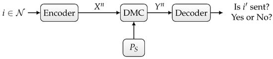
Figure 1.
Discrete memoryless channel with random state.
In the sequelae, we distinguish three scenarios:
- Randomized ID over the state-dependent channel , as depicted in Figure 1,
- Deterministic or randomized ID over the state-dependent channel in the presence of noiseless feedback between the sender and the receiver, as depicted in Figure 2,
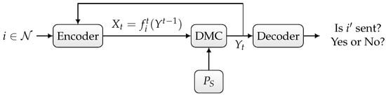 Figure 2. Discrete memoryless channel with random state and noiseless feedback.
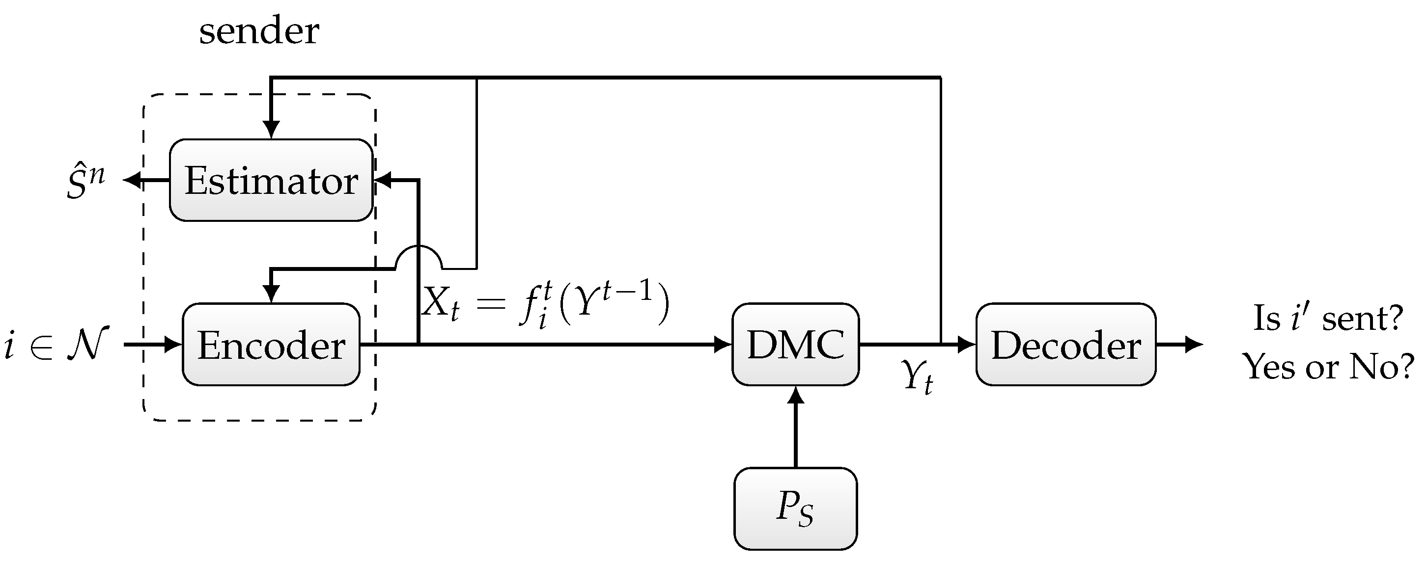
 - Joint deterministic or randomized ID and sensing, in which the sender wishes to simultaneously send an identity to the receiver and sense the channel state sequence based on the output of the noiseless feedback link, as depicted in Figure 3.
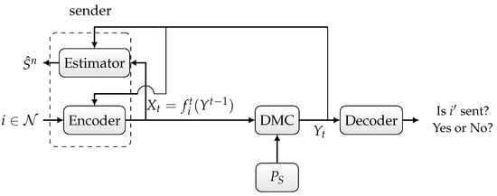 Figure 3. State-dependent channel with noiseless feedback.
First, we define randomized ID codes for the state-dependent channel defined above.
Definition 1.
An randomized ID code with for channel is a family of pairs with
such that the errors of the first kind and the second kind are bounded as follows:
In the following, we define the achievable ID rate and ID capacity for our system model.
Definition 2.
- 1.
- The rate R of a randomized ID code for the channel is bits.
- 2.
- The ID rate R for is said to be achievable if for there exists an such that for all there exists an randomized ID code for .
- 3.
- The randomized ID capacity of the channel is the supremum of all achievable rates.
The following theorem characterizes the randomized ID capacity of the state-dependent channel when the state information is known to neither the sender nor the receiver.
Theorem 1.
The randomized ID capacity of the channel is provided by
where denotes the Shannon transmission capacity of .
Proof.
The proof of Theorem 1 follows from Theorem 6.6.4 of [26] and Equation (7.2) of [27]. Because the channel satisfies the strong converse property [26], the randomized ID capacity of coincides with its Shannon transmission capacity determined in [27]. □
Now, we consider the second scenario depicted in Figure 2. Let further denote the output of the noiseless backward (feedback) channel:
In the following, we define a deterministic and randomized ID feedback code for the state-dependent channel .
Definition 3.
An deterministic ID feedback code with for the channel is characterized as follows. The sender wants to send an ID message that is encoded by the vector-valued function
where and for . At , the sender sends . At , the sender sends . The decoding sets should satisfy the following inequalities:
Definition 4.
An randomized ID feedback code
with for the channel is characterized as follows. The sender wants to send an ID message that is encoded by the probability distribution
where denotes the set of all n-length functions as . The decoding sets , should satisfy the following inequalities:
Definition 5.
- 1.
- The rate R of a (deterministic/randomized) ID feedback code for the channel is bits.
- 2.
- The (deterministic/randomized) ID feedback rate R for is said to be achievable if for there exists an such that for all there exists a (deterministic/randomized) ID feedback code for .
- 3.
- The (deterministic/randomized) ID feedback capacity / of the channel is the supremum of all achievable rates.
It has been demonstrated in [26] that noise increases the ID capacity of the DMC in the case of feedback. Intuitively, noise is considered a source of randomness, i.e., a random experiment for which outcome is provided to the sender and receiver via the feedback channel. Thus, adding a perfect feedback link enables the realization of a correlated random experiment between the sender and the receiver. The size of this random experiment can be used to compute the growth of the ID rate. This result has been further emphasized in [15,28], where it has been shown that the ID capacity of the Gaussian channel with noiseless feedback is infinite. This is because the authors of [15,28] provided a coding scheme that generates infinite common randomness between the sender and the receiver. Here, we want to investigate the effect of feedback on the ID capacity of the system model depicted in Figure 2. Theorem 2 characterizes the ID feedback capacity of the state-dependent channel with noiseless feedback. The proof of Theorem 2 is provided in Section 3.
Theorem 2.
If , then the deterministic ID feedback capacity of is provided by
Theorem 3.
If , then the randomized ID feedback capacity of is provided by
Remark 1.
It can be shown that the same ID feedback capacity formula holds if the channel state is known to either the sender or the receiver. This is because we achieve the same amount of common randomness as in the scenario depicted in Figure 2. Intuitively, the channel state is an additional source of randomness that we can take advantage of.
Now, we consider the third scenario depicted in Figure 3, where we want to jointly identify and sense the channel state. The sender comprises an encoder that sends a symbol for each identity and delayed feedback output along with a state estimator that outputs an estimation sequence based on the feedback output and input sequence. We define the per-symbol distortion as follows:
where is a distortion function and the expectation is over the joint distribution of conditioned by the ID message .
Definition 6.
- 1.
- An ID rate–distortion pair for is said to be achievable if for every there exists an such that for all there exists an (deterministic/randomized) ID code for and if for all .
- 2.
- The deterministic ID capacity–distortion function is defined as the supremum of R such that is achievable.
Without loss of generality, we choose the following deterministic estimation function :
where is an estimator that maps a channel input–feedback output pair to a channel state. If there exist several functions , we choose one randomly. We define the minimal distortion function for each input symbol as in [29]:
and the minimal distortion function for each input distribution as
In the following, we establish the ID capacity–distortion function defined above.
Theorem 4.
The deterministic ID capacity–distortion function of the state-dependent channel depicted in Figure 3 is provided by
where the set is provided by
We now turn our attention to a randomized encoder. In the following, we derive the ID capacity–distortion function of the state-dependent channel under the assumption of randomized encoding.
Theorem 5.
The randomized ID capacity–distortion function of the state-dependent channel is provided by
where the set is provided by
Remark 2.
Randomized encoding achieves higher rates than deterministic encoding. This is because we are combining two sources of randomness: local randomness used for the encoding, and shared randomness generated via the noiseless feedback link. The result is analogous to randomized ID over DMCs in the presence of noiseless feedback, as studied in [14].
3. Proof of the Main Results
In this section, we provide the proofs of Theorems 2–5.
3.1. Direct Proof of Theorem 2
Proof.
We consider an average channel provided by
The DMC is obtained by averaging the DMCs over the state. Now, it suffices to show that is an achievable ID feedback rate for the average channel . The deterministic ID feedback capacity of the average channel can be determined by applying Theorem 1 of [28] on . If the transmission capacity of is positive, we have
This completes the direct proof of Theorem 2. □
3.2. Converse Proof of Theorem 2
Proof.
For the converse proof, we use the techniques of [14] for deterministic ID over DMCs with noiseless feedback. We first extend Lemma 3 of [14] (image size for a deterministic feedback strategy) to the deterministic ID feedback code for described in Definition 3. □
Lemma 1.
For any feedback strategy and any , we have
where is provided by
where
Proof.
We use a similar idea as for the proof of Lemma 3 of [14]. Let be defined as follows:
It then follows from the definition of that . It remains to show that
For and a fixed feedback strategy , we have
Let the RV be defined as follows:
We have
Now, we want to establish a lower bound on . It suffices to find a lower bound on the expression in (40). Let the RV be defined as follows:
It can be shown that
Furthermore, we have
It can be shown that for ,
It follows from the definition of the RV in (41) that
where follows from the definition of in (27) and follows from (52).
It can be verified that
Therefore, we can apply Chebyshev’s inequality and obtain
where follows the definition of in (28). This completes the proof of Lemma 1. □
We establish an upper bound on the deterministic ID feedback rate for the channel model using Lemma 1. Let be an deterministic ID feedback code for channel with , and let be chosen such that
For each feedback strategy , we define the set that satisfies (26). For , we have
where follows from the union bound, follows from the definition of the ID feedback code and from (26), and follows from (61). Similarly, from the definition of the ID feedback code
from (26) and (61), for and it follows that
As the error of the second kind is smaller than , all the sets are distinct. Therefore, any deterministic ID feedback code for channel with has an associated deterministic ID feedback code , where and the set satisfies (26) . Thus, per Lemma 1, the cardinality N of the deterministic ID feedback code is upper-bounded as follows:
This completes the converse proof of Theorem 2.
3.3. Direct Proof of Theorem 3
Proof.
Similarly, we can consider the average channel defined in (23). It is sufficient to show that is an achievable randomized ID feedback rate for the average channel . The randomized ID feedback capacity of the average channel can be obtained by applying Theorem 2 of [28] on . If the transmission capacity of is positive, then we have
This completes the direct proof of Theorem 3. □
3.4. Converse Proof of Theorem 3
Proof.
We first extend Lemma 4 of [14] (image size for a randomized feedback strategy) to the randomized ID feedback code for . □
Lemma 2.
For any randomized feedback strategy over all n-length feedback encoding sets and any ,
where is provided by
where , .
Proof.
We use a similar idea as for the proof of Lemma 4 in [14]. We define the set as follows:
From the definition of , we have
□
Then, it is sufficient to show that . Let the RV be defined as follows:
where and is the set of all mapping . We have
Now, for any , we consider
Similarly, for all , we define the RV . It has been shown in (44) and (48) that and . Combining (80) and (83), we have
Assuming for all , we can apply Chebyshev’s inequality to obtain
Replacing in the converse proof of Theorem 2 with the corresponding as outlined in Lemma 2 completes the converse proof of Theorem 3.
3.5. Direct Proof of Theorem 4
3.5.1. Coding Scheme
Proof.
To some extent, we use the same coding scheme elaborated in [14]. We choose the blocklength as . Let be some symbol in . Regardless of which identity we want to identify, the sender first sends the sequence over the state-dependent channel . The received sequence becomes known to the sender (estimator and encoder) via the noiseless feedback link. The feedback provides the sender and receiver with knowledge of the outcome of the correlated random experiment . □
3.5.2. Common Randomness Generation
We want to generate uniform common randomness, as it is the most convenient form of common randomness [17]; therefore, we convert our correlated random experiment to a uniform one . For , the set is provided by
where is defined as follows.
Definition 7.
Let be the set of stochastic matrices . Let such that
For , the distance is defined as
Here, denotes the average channel defined by
We introduce the following lemmas.
Lemma 3
([30]).
Let be emitted by the DMS and let such that . Then, for every there exist and such that for we have
Lemma 4
([30]).
Let be emitted by the DMS and let . For every , there exist a and such that for we have
- 1.
- ,
- 2.
- ,
- 3.
- If , and if , then
Lemma 5
([31]).
Let be i.i.d. RVs taking values in with mean μ; then, with we have
where .
For arbitrary , we define and by
It is clear that is a non-decreasing function, because for arbitrary . Letting , we have
It follows from Lemma 4 that is essentially uniform on . Let the set be denoted by . Per Lemma 3, we have
As mentioned earlier, we have . This quantity is the size of the correlated random experiment , which determines the growth of the ID rate. Let be an code, where for each . We concatenate the sequence and the transmission code to build an ID feedback code for . We now have . The concatenation is performed using the coloring functions . We choose a suitable set of coloring functions at random. Every coloring function corresponds to an ID message i and maps each element to an element in a smaller set . After has been received by the sender (encoder and estimator) via the noiseless feedback channel, if is available, then the encoder sends . Note that we define an encoding strategy for each coloring function , as presented in Definition 4. If , then an error is declared. This error probability goes to zero as n goes to infinity, as computed in (102). For a fixed family of maps and for each , we define the decoding sets .
3.5.3. Error Analysis
Next, we analyze the maximal error performance of the deterministic ID feedback code. For our analysis of the error of the first kind, we choose a fixed set . The error of the first kind is upper-bounded by
where follows from the memorylessness property of the channel and the union bound, while follows from Lemma 3 and the definition of the transmission code .
In order to achieve a small error of the second kind, we choose suitable maps randomly. For , , let be independent RVs such that
Let be a realization of . For each , we define the RVs analogously to Section IV of [14]:
The are also independent for every . The expectation of is computed as follows:
Because the are i.i.d. for all , we can apply Hoeffding’s inequality Lemma 5 to obtain the following Lemma.
Lemma 6.
For , for each channel with , while for each we have
We can derive an upper bound on the error of the second kind for those values of satisfying Lemma 6:
where follows from the union bound, follows from the memorylessness property of the channel and the union bound, follows from Lemma 3 along with the definition of the transmission code and the definition of the set in (90), and follows from Lemma 6.
We repeatedly perform the same analysis of the error of the second kind for all pairs . For simplicity of notation, we denote the error of the second kind between the pair by . We have
where follows from the union bound, Equation (122) and Lemma 6. It is verifiable that we can construct an ID feedback code for with cardinality N satisfying
and with an error of the second kind upper-bounded as in (122).
The next step in the proof is dedicated to the state estimator. The per-symbol distortion defined in (15) can be rewritten as follows:
This completes the direct proof of Theorem 4.
3.6. Converse Proof of Theorem 4
Proof.
For the converse proof, we use the techniques for deterministic ID for as described in Section 3.2. We first extend Lemma 1 to the joint deterministic ID and sensing problem. □
Lemma 7.
For any feedback strategy which satisfies the per-symbol distortion constraint as described in (17), i.e., for all , and for any , we have
where is provided by
where
Proof.
Let be defined as follows:
Define an RV . Per (40), we have
Similarly, for all , we define an RV . It has been shown in (44) and (48) that and .
Moreover, for all and for all , we have
By combining (139) and (142), we have
This completes the proof of Lemma 7 □
The subsequent steps in the proof are identical to Section 3.2.
3.7. Direct Proof of Theorem 5
Proof.
For the direct proof of this theorem, we follow a code construction similar to that presented in [14], with one key difference, namely, that we optimize only over input distributions that satisfy the per-symbol constraint . □
3.7.1. Coding Scheme
We construct a randomized ID code with blocklength by concatenating two transmission codes, which is described in detail later. The first n symbols are allocated for generation of common randomness. We employ a distribution
where the maximization is performed over distributions subject to the constraint . Regardless of which identity we want to identify, the sender first sends n symbols with respect to the distribution over the state-dependent channel . The received sequence becomes known to the sender (estimator and encoder) via the noiseless feedback link. The feedback provides the sender and the receiver with knowledge of the outcome of the correlated random experiment .
3.7.2. Common Randomness Generation
Similar to the deterministic coding scheme, we want to generate uniform common randomness. Therefore, we convert our correlated random experiment
to a uniform one . For , the set is provided by
Per Lemma 4, we can obtain the following corollary.
Corollary 1.
Let be emitted by the DMS and let . For every , there exist a and such that for we have:
- 1.
- ,
- 2.
- ,
- 3.
- If , and if , then
Therefore, we have . The sender generates randomness according to the random experiment . Asymptotically, the error probability of goes to zero. Similar to the deterministic scheme, we prepare the coloring functions . The last symbols are used to transmit using a standard transmission code , where for each . The probability distribution for encoding is defined as and the decoding region is provided by .
3.7.3. Error Analysis
Subsequently, for all , the error of the first kind is upper-bounded by
where follows from the union bound and follows from Corollary 1. Furthermore, for all with , the probability of the error of the second kind should be asymptotically upper-bounded by . Without loss of generality, we fix , and examine the error probability :
where follows from the union bound, follows from the memoryless channel and the union bound, follows from Lemma 3 along with the definition of the transmission code and the definition of the set in (90), and follows from Corollary 1.
We repeatedly perform the same analysis of the error of the second kind for all pairs . It is verifiable that we can construct a randomized ID feedback code for with cardinality N satisfying
and with errors of the first and second kind that are upper-bounded as in (11) and (12), respectively.
Finally the state estimator is checked. The per-symbol distortion defined in (15) can be rewritten as follows:
This completes the direct proof of Theorem 5.
3.8. Converse Proof of Theorem 5
Proof.
We first extend Lemma 2 to the joint randomized ID and sensing problem. □
Lemma 8.
For any randomized feedback strategy over all n-length feedback encoding sets which satisfies the per symbol distortion constraint as described in (142), i.e., for all , and for any , we have
where is provided by
where , .
Proof.
Define a set as follows:
Define an auxiliary RV as follows:
Then, per (80), we have
Similarly, for any , we can examine
By applying Chebyshev’s inequality, we complete the proof of Lemma 8. □
The subsequent steps in the proof are the same as in Section 3.6.
4. Average Distortion
In addition to the per-symbol distortion constraint, an alternative and more flexible distortion constraint is the average distortion. This approach is valuable because it relaxes the per-symbol fidelity requirement, allowing for minor variations in individual symbol quality as long as the overall average distortion remains below a specified threshold. As defined in [32], the average distortion for a sequence of symbols is provided by
This metric captures the average quality of the reconstructed sequence, making it suitable for applications where consistent strict fidelity for each symbol is not essential but where the overall fidelity of the transmission needs to remain within acceptable limits.
In the case of a deterministic ID code, the average distortion can be expressed in a more detailed form as
Using the code construction method from Section 3.5 along with the minimum distortion condition defined in (17), we propose the following theorem, which provides a lower bound on the deterministic ID capacity–distortion function for a state-dependent channel under an average distortion constraint.
Theorem 6.
The deterministic ID capacity–distortion function with average distortion constraint of the state-dependent channel is lower-bounded as follows:
where the set is provided by
Despite the practical implications of this result, proving a converse theorem for this bound remains an open problem.
5. Conclusions and Discussion
In this work, we have studied the problem of joint ID and channel state estimation over a DMC with i.i.d. state sequences where the sender simultaneously sends an identity and senses the state via a strictly causal channel output. After establishing the capacity on the corresponding ID capacity–distortion function, it emerges that sensing can increase the ID capacity. In the proof of our theorem, we noticed that the generation of common randomness is a key tool for achieving a high ID rate. The common randomness generation is helped by feedback. The ID rate can be further increased by adding local randomness at the sender.
Our framework closely mirrors the one described in [23], with the key distinction being that we utilize an identification scheme instead of the classical transmission scheme. We want to simultaneously identify the sent message and estimate the channel’s state. As noted in the results of [23], the capacity–distortion function is consistently smaller than the transmission capacity of the state-dependent DMC except when the distortion is infinite. This observation aligns with expectations for the message transmission scheme, as the optimization is performed over a constrained input set defined by the distortion function. However, this does not directly apply to the ID scheme. An interesting aspect is that the capacity–distortion function for the deterministic encoding case scales double exponentially with the blocklength, as highlighted in Theorem 4. However, the ID capacity of the state-dependent DMC with deterministic encoding scales only exponentially with the blocklength. This is because feedback significantly enhances the ID capacity, enabling double-exponential growth of the ID capacity for the state-dependent DMC, as established in Theorem 2. This contrasts sharply with the message transmission scheme, where feedback does not increase the capacity of a DMC. Introducing an estimator into our framework naturally reduces the ID capacity compared to the scenario with feedback but without an estimator. This reduction occurs because the optimization is performed over a constrained input set defined by the distortion function. Nevertheless, the capacity–distortion function remains higher than in the case without feedback and without an estimator. This difference underscores a unique characteristic of the ID scheme, highlighting its distinct scaling behavior and potential advantages in certain scenarios.
We consider two cases, namely, deterministic and randomized identification. For a transmission system without sensing, it was shown in [1,3] that the number of messages grows exponentially, i.e., .
Remarkably, Theorem 4 demonstrates that by incorporating sensing, the growth rate of the number of messages becomes double exponential (); this result is notable, and closely parallels the findings on identification with feedback in [14].
In the case of randomized identification, Theorem 5 shows that the capacity is also improved by incorporating sensing. However, in both the deterministic and randomized settings, the scaling remains double exponential.
One application of message identification is in control and alarm systems [10,33]. For instance, it has been shown that identification codes can be used for status monitoring in digital twins [34]. In this context, our results demonstrate that incorporating a sensing process can significantly enhance the capacity.
Another potential application of our framework is molecular communication, where nanomachines use identification codes to determine when to perform specific actions such as drug delivery [35]. In this context, sensing the position of the nanomachines can enhance the communication rate. For such scenarios, it is also essential to explore alternative channel models such as the Poisson channel.
Furthermore, it is clear that in other applications it would be necessary to consider different distortion functions.
In the future, it would be interesting to apply the method proposed in this paper to other distortion functions. Furthermore, in practical scenarios, there are models where the the sensing is performed either additionally or exclusively by the receiver. This suggests the need to study a wider variety of system models. For wireless communications, the Gaussian channel is more practical and widely applicable. Therefore, it would be valuable to extend our results to the Gaussian case (JIDAS scheme with a Gaussian channel as the forward channel). It has been shown in [15,28] that the ID capacity of a Gaussian channel with noiseless feedback is infinite. Interestingly, the ID capacity of a Gaussian channel with noiseless feedback remains infinite regardless of the scaling used for the rate, e.g., double exponential, triple exponential, etc. By introducing an estimator, we conjecture that the same results will hold, leading to an infinite capacity–distortion function. Thus, considering scenarios with noisy feedback is more practical for future research.
Author Contributions
Writing—original draft preparation, W.L. and Y.Z.; supervision, C.D. and H.B. All authors have read and agreed to the published version of the manuscript.
Funding
The authors acknowledge financial support by the Federal Ministry of Education and Research of Germany (BMBF) through the “Souverän. Digital. Vernetzt.” programme, joint project “6G-life”, project identification number 16KISK002. H. Boche and W. Labidi were further supported in part by the BMBF within the national initiative on Post-Shannon Communication (NewCom) under Grant 16KIS1003K and within the national initiative on molecular communication (IoBNT) under grant 16KIS1988. C. Deppe was further supported in part by the BMBF within the national initiative on Post-Shannon Communication (NewCom) under Grant 16KIS1005. C. Deppe, W. Labidi and Y. Zhao were supported by the DFG within the projects DE1915/2-1 and BO 1734/38-1.
Institutional Review Board Statement
Not applicable.
Data Availability Statement
The original contributions presented in this study are included in the article. Further inquiries can be directed to the corresponding author.
Acknowledgments
This work has been presented in part at the IEEE International Symposium on Information Theory 2023 (ISIT 2023) [32].
Conflicts of Interest
The authors declare no conflicts of interest.
References
- Ahlswede, R.; Dueck, G. Identification via channels. IEEE Trans. Inf. Theory 1989, 35, 15–29. [Google Scholar] [CrossRef]
- Shannon, C.E. A mathematical theory of communication. Bell Syst. Tech. J. 1948, 27, 379–423. [Google Scholar] [CrossRef]
- Salariseddigh, M.J.; Pereg, U.; Boche, H.; Deppe, C. Deterministic Identification over Channels with Power Constraints. IEEE Trans. Inf. Theory 2022, 68, 1–24. [Google Scholar] [CrossRef]
- Ahlswede, R.; Cai, N. Identification without randomization. IEEE Trans. Inf. Theory 1999, 45, 2636–2642. [Google Scholar] [CrossRef]
- Moulin, P. The role of information theory in watermarking and its application to image watermarking. Signal Process. 2001, 81, 1121–1139. [Google Scholar] [CrossRef]
- Ahlswede, R. Watermarking Identification Codes with Related Topics on Common Randomness. In Identification and Other Probabilistic Models: Rudolf Ahlswede’s Lectures on Information Theory 6; Ahlswede, A., Althöfer, I., Deppe, C., Tamm, U., Eds.; Springer International Publishing: Cham, Switzerland, 2021; pp. 271–325. [Google Scholar] [CrossRef]
- Steinberg, Y.; Merhav, N. Identification in the presence of side information with application to watermarking. IEEE Trans. Inf. Theory 2001, 47, 1410–1422. [Google Scholar] [CrossRef]
- Lu, Y. Industry 4.0: A survey on technologies, applications and open research issues. J. Ind. Inf. Integr. 2017, 6, 1–10. [Google Scholar] [CrossRef]
- Fettweis, G.; Boche, H. 6G: The Personal Tactile Internet—And Open Questions for Information Theory. IEEE BITS Inf. Theory Mag. 2021, 1, 71–82. [Google Scholar] [CrossRef]
- Cabrera, J.; Boche, H.; Deppe, C.; Schaefer, R.F.; Scheunert, C.; Fitzek, F. 6G and the Post-Shannon-Theory. In Shaping Future 6G Networks: Needs, Impacts and Technologies; Bertin, E., Crespi, N., Magedanz, T., Eds.; Wiley-Blackwell: Oxford, UK, 2021. [Google Scholar] [CrossRef]
- Fettweis, G.; Boche, H. On 6G and trustworthiness. Commun. ACM 2022, 65, 48–49. [Google Scholar] [CrossRef]
- Ahlswede, R.; Zhang, Z. New directions in the theory of identification via channels. IEEE Trans. Inf. Theory 1995, 41, 1040–1050. [Google Scholar] [CrossRef]
- Labidi, W.; Deppe, C.; Boche, H. Secure Identification for Gaussian Channels. In Proceedings of the ICASSP 2020—2020 IEEE International Conference on Acoustics, Speech and Signal Processing (ICASSP), Barcelona, Spain, 4–8 May 2020; pp. 2872–2876. [Google Scholar] [CrossRef]
- Ahlswede, R.; Dueck, G. Identification in the presence of feedback-a discovery of new capacity formulas. IEEE Trans. Inf. Theory 1989, 35, 30–36. [Google Scholar] [CrossRef]
- Labidi, W.; Boche, H.; Deppe, C.; Wiese, M. Identification over the Gaussian Channel in the presence of feedback. In Proceedings of the 2021 IEEE International Symposium on Information Theory (ISIT), Melbourne, Australia, 12–20 July 2021; pp. 278–283. [Google Scholar] [CrossRef]
- Ahlswede, R. General theory of information transfer: Updated. Discret. Appl. Math. 2008, 156, 1348–1388. [Google Scholar] [CrossRef]
- Ahlswede, R.; Csiszar, I. Common randomness in information theory and cryptography. II. CR capacity. IEEE Trans. Inf. Theory 1998, 44, 225–240. [Google Scholar] [CrossRef]
- Proceedings of the 1st IEEE International Online Symposium on Joint Communications and Sensing; IEEE: Piscataway, NJ, USA, 2021; Available online: https://www.proceedings.com/58212.html (accessed on 18 November 2024).
- Sturm, C.; Wiesbeck, W. Waveform Design and Signal Processing Aspects for Fusion of Wireless Communications and Radar Sensing. Proc. IEEE 2011, 99, 1236–1259. [Google Scholar] [CrossRef]
- Bliss, D.W. Cooperative radar and communications signaling: The estimation and information theory odd couple. In Proceedings of the 2014 IEEE Radar Conference, Cincinnati, OH, USA, 9–23 May 2014; pp. 50–55. [Google Scholar] [CrossRef]
- Bica, M.; Huang, K.W.; Mitra, U.; Koivunen, V. Opportunistic Radar Waveform Design in Joint Radar and Cellular Communication Systems. In Proceedings of the 2015 IEEE Global Communications Conference (GLOBECOM), San Diego, CA, USA, 6–10 December 2015; pp. 1–7. [Google Scholar] [CrossRef]
- Huang, K.W.; Bică, M.; Mitra, U.; Koivunen, V. Radar waveform design in spectrum sharing environment: Coexistence and cognition. In Proceedings of the 2015 IEEE Radar Conference (RadarCon), Arlington, VA, USA, 10–15 May 2015; pp. 1698–1703. [Google Scholar] [CrossRef]
- Kobayashi, M.; Caire, G.; Kramer, G. Joint State Sensing and Communication: Optimal Tradeoff for a Memoryless Case. In Proceedings of the 2018 IEEE International Symposium on Information Theory (ISIT), Vail, CO, USA, 17–22 June 2018; pp. 111–115. [Google Scholar] [CrossRef]
- Choudhuri, C.; Kim, Y.H.; Mitra, U. Causal State Communication. IEEE Trans. Inf. Theory 2013, 59, 3709–3719. [Google Scholar] [CrossRef]
- Chiu, S.E.; Ronquillo, N.; Javidi, T. Active Learning and CSI Acquisition for mmWave Initial Alignment. IEEE J. Sel. Areas Commun. 2019, 37, 2474–2489. [Google Scholar] [CrossRef]
- Han, T.S. Information-Spectrum Methods in Information Theory; Stochastic Modelling and Applied Probability; Springer: Berlin/Heidelberg, Germany, 2014. [Google Scholar] [CrossRef]
- El Gamal, A.; Kim, Y.H. Network Information Theory; Cambridge University Press: Cambridge, UK, 2011. [Google Scholar] [CrossRef]
- Wiese, M.; Labidi, W.; Deppe, C.; Boche, H. Identification over Additive Noise Channels in the Presence of Feedback. IEEE Trans. Inf. Theory 2022, 69, 6811–6821. [Google Scholar] [CrossRef]
- Zhang, W.; Vedantam, S.; Mitra, U. Joint Transmission and State Estimation: A Constrained Channel Coding Approach. IEEE Trans. Inf. Theory 2011, 57, 7084–7095. [Google Scholar] [CrossRef]
- Csiszár, I.; Körner, J. Information Theory: Coding Theorems for Discrete Memoryless Systems; Cambridge University Press: Cambridge, UK, 2011. [Google Scholar] [CrossRef]
- Hoeffding, W. On Probabilities of Large Deviations. In The Collected Works of Wassily Hoeffding; Springer: New York, NY, USA, 1994; pp. 473–490. [Google Scholar] [CrossRef]
- Labidi, W.; Deppe, C.; Boche, H. Joint identification and sensing for discrete memoryless channels. In Proceedings of the 2023 IEEE International Symposium on Information Theory (ISIT), Taipei, Taiwan, 25–30 June 2023; pp. 442–447. [Google Scholar] [CrossRef]
- Bringer, J.; Chabanne, H. Code Reverse Engineering Problem for Identification Codes. IEEE Trans. Inf. Theory 2012, 58, 2406–2412. [Google Scholar] [CrossRef]
- von Lengerke, C.; Cabrera, J.A.; Fitzek, F.H.P. Identification Codes for Increased Reliability in Digital Twin Applications over Noisy Channels. In Proceedings of the 2023 IEEE International Conference on Metaverse Computing, Networking and Applications (MetaCom), Kyoto, Japan, 26–28 June 2023; pp. 550–557. [Google Scholar] [CrossRef]
- Labidi, W.; Deppe, C.; Boche, H. Information-Theoretical Analysis of Event-Triggered Molecular Communication. In Proceedings of the European Wireless 2024, Brno, Czech Republic, 9–11 September 2024. [Google Scholar]

Disclaimer/Publisher’s Note: The statements, opinions and data contained in all publications are solely those of the individual author(s) and contributor(s) and not of MDPI and/or the editor(s). MDPI and/or the editor(s) disclaim responsibility for any injury to people or property resulting from any ideas, methods, instructions or products referred to in the content. |
© 2024 by the authors. Licensee MDPI, Basel, Switzerland. This article is an open access article distributed under the terms and conditions of the Creative Commons Attribution (CC BY) license (https://creativecommons.org/licenses/by/4.0/).