
Probabilistic Estimation and Control of Dynamical Systems Using Particle Filter with Adaptive Backward Sampling


Abstract
1. Introduction
2. Methods
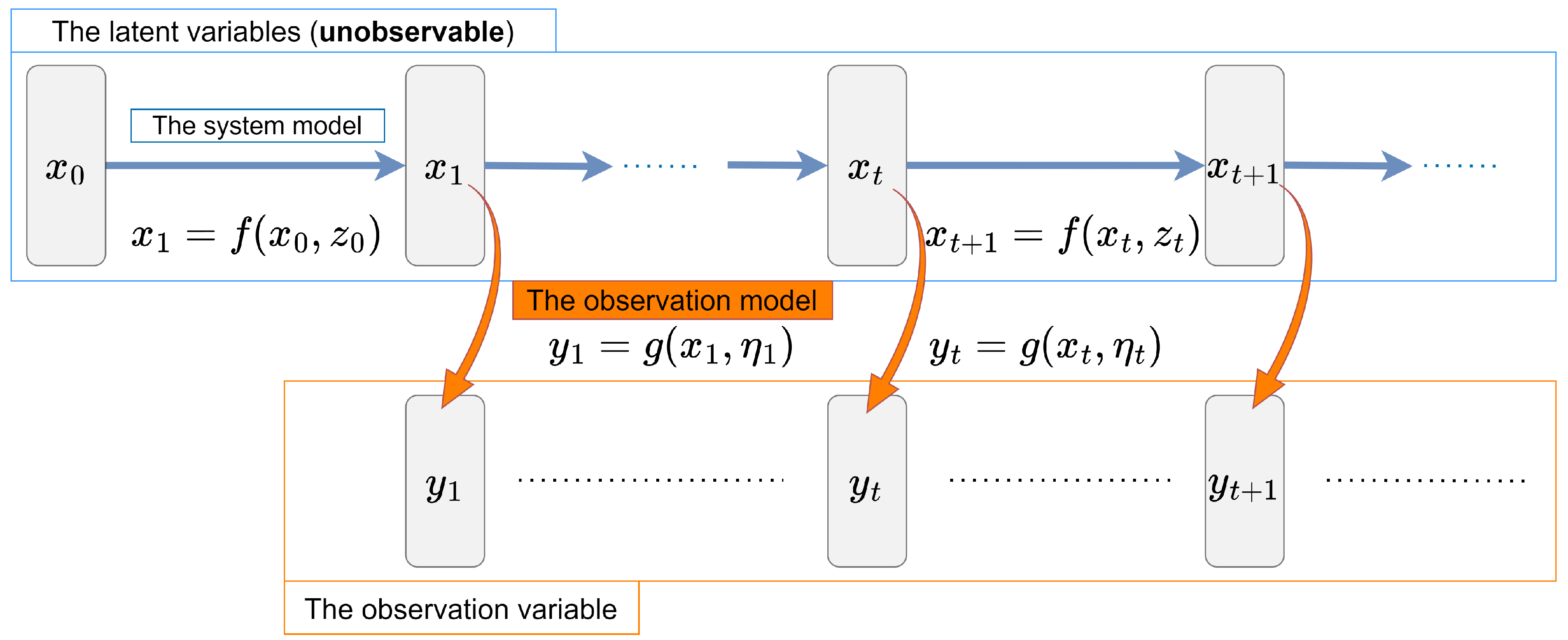
2.1. Formulation of State-Space Model
2.2. Estimation of the Hidden State
2.3. Estimation of the Parameter
2.3.1. EM Algorithm
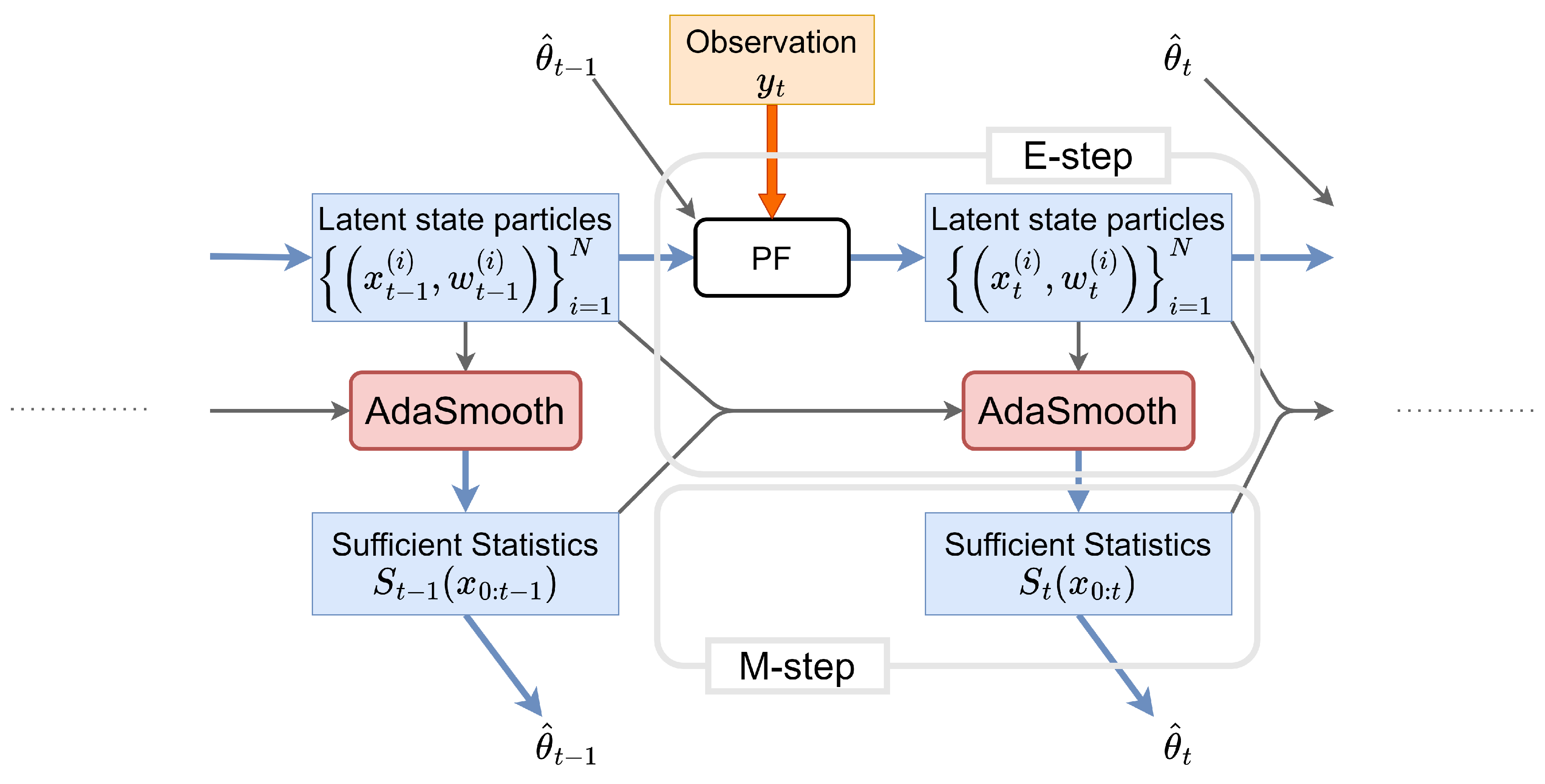
2.3.2. AdaSmooth-Based Online EM Algorithm
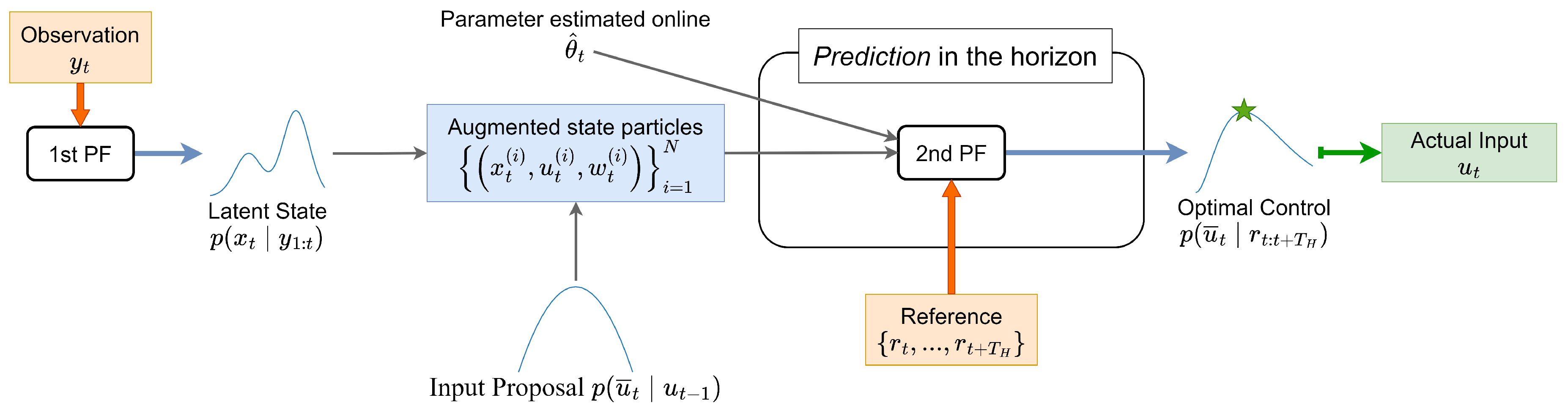
2.4. Control Strategy for the Dynamics
3. Experiments
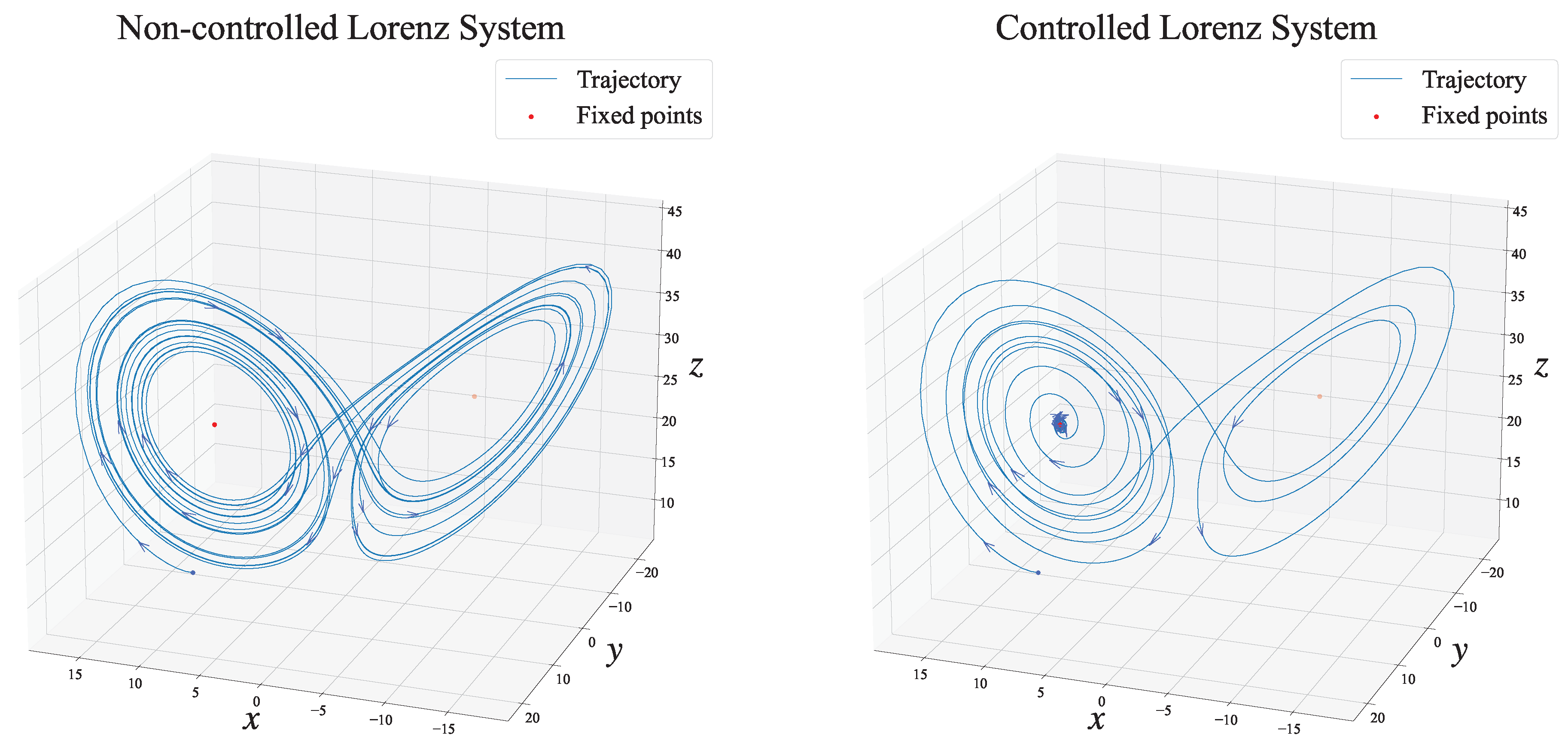
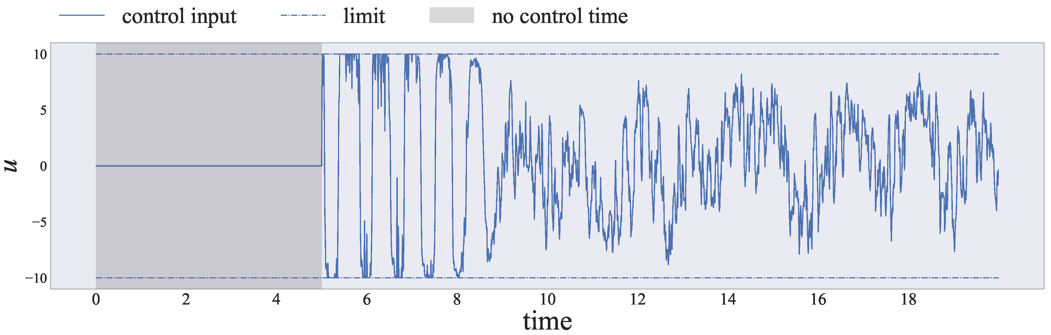
3.1. Application to Chaotic Lorenz System
3.1.1. Formulation of State-Space Model
3.1.2. Derivation of Online EM Algorithm
3.1.3. Formulation of the Augmented State-Space Model for Control
3.1.4. Settings
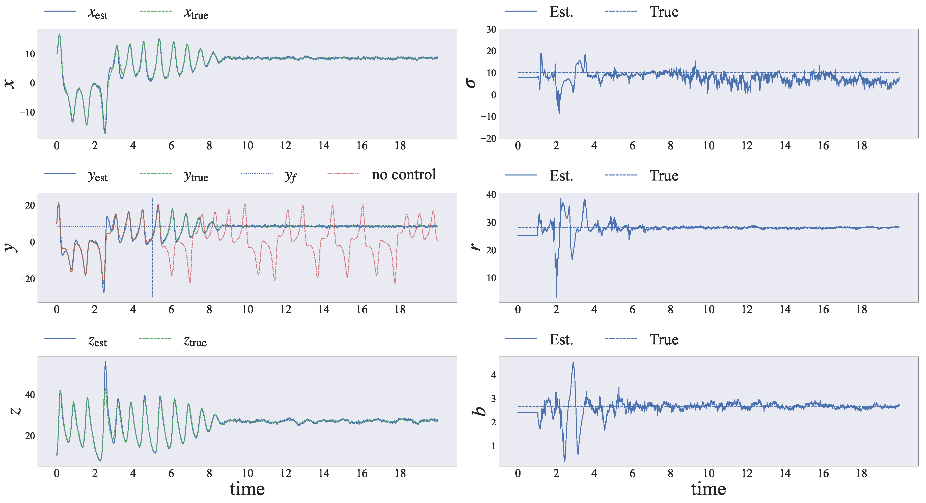
3.1.5. Results
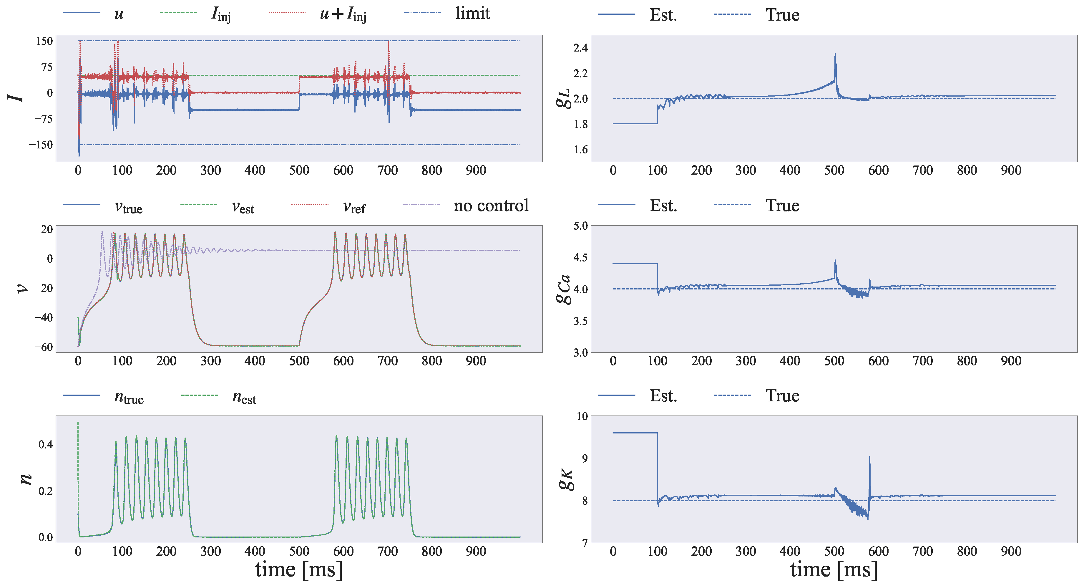
3.2. Application to Morris–Lecar Neuron Model
3.2.1. Formulation of State-Space Model
3.2.2. Derivation of Online EM Algorithm
3.2.3. Formulation of the Augmented State-Space Model for Control
3.2.4. Settings
3.2.5. Results
4. Conclusions
Author Contributions
Funding
Data Availability Statement
Conflicts of Interest
Abbreviations
| SSM | State-space model |
| PF | Particle filter |
| EM algorithm | Expectation-maximization algorithm |
| AdaSmooth | Adaptive smoothing |
| MPC | Model predictive control |
| PF-MPC | Particle filter-based model predictive control |
References
- Cheng, S.; Quilodrán-Casas, C.; Ouala, S.; Farchi, A.; Liu, C.; Tandeo, P.; Fablet, R.; Lucor, D.; Iooss, B.; Brajard, J.; et al. Machine learning with data assimilation and uncertainty quantification for dynamical systems: A review. IEEE/CAA J. Autom. Sin. 2023, 10, 1361–1387. [Google Scholar] [CrossRef]
- Inoue, H.; Hukushima, K.; Omori, T. Estimating distributions of parameters in nonlinear state space models with replica exchange particle marginal metropolis-hastings method. Entorpy 2022, 24, 115. [Google Scholar] [CrossRef] [PubMed]
- Ito, M.; Kuwatani, T.; Oyanagi, R.; Omori, T. Data-driven analysis of nonlinear heterogeneous reactions through sparse modeling and Bayesian statistical approaches. Entropy 2021, 23, 824. [Google Scholar] [CrossRef] [PubMed]
- Omori, T.; Kuwatani, T.; Okamoto, A.; Hukushima, K. Bayesian inversion analysis of nonlinear dynamics in surface heterogeneous reactions. Phys. Rev. E 2016, 94, 033305. [Google Scholar] [CrossRef] [PubMed]
- Ditlevsen, S.; Samson, A. Estimation in the partially observed stochastic Morris–Lecar neuronal model with particle filter and stochastic approximation methods. Ann. Appl. Stat. 2014, 8, 674–702. [Google Scholar] [CrossRef]
- Azza, L.J.; Crompton, D.; D’Eleuterio, G.M.T.; Skinner, F.; Lankarany, M. Adaptive unscented Kalman filter for neuronal state and parameter estimation. J. Comput. Neurosci. 2023, 51, 223–237. [Google Scholar] [CrossRef]
- Chan, J.C.; Strachan, R.W. Bayesian state space models in macroeconometrics. J. Econ. Surv. 2023, 37, 58–75. [Google Scholar] [CrossRef]
- Newman, K.; King, R.; Elvira, V.; de Valpine, P.; McCrea, R.; Morgan, B.J.T. State-space models for ecological time-series data: Practical model-fitting. Methods Ecol. Evol. 2023, 14, 26–42. [Google Scholar] [CrossRef]
- Ahwiadi, M.; Wang, W. An enhanced particle filter technology for battery system state estimation and RUL prediction. Measurement 2022, 191, 110817. [Google Scholar] [CrossRef]
- El-Dalahmeh, M.; Al-Greer, M.; El-Dalahmeh, M.; Bashir, I. Physics-based model informed smooth particle filter for remaining useful life prediction of lithium-ion battery. Measurement 2023, 214, 112838. [Google Scholar] [CrossRef]
- Kitagawa, G. A Monte Carlo filtering and smoothing method for non-Gaussian nonlinear state space models. In Proceedings of the 2nd U.S.-Japan Joint Seminar on Statistical Time Series, Honolulu, HI, USA, 25–29 January 1993. [Google Scholar]
- Doucet, A.; Freitas, N.; Gordon, N. Sequenatial Monte Carlo Methods in Practice; Springer: Berlin/Heidelberg, Germany, 2001. [Google Scholar]
- Wills, A.G.; Schön, T.B. Sequential Monte Carlo: A unified review. Annu. Rev. Control Robot. Auton. Syst. 2023, 6, 159–182. [Google Scholar] [CrossRef]
- Kantas, N.; Doucet, A.; Singh, S.S.; Maciejowski, J.; Chopin, N. On particle methods for parameter estimation in state-space models. Stat. Sci. 2015, 30, 328–351. [Google Scholar] [CrossRef]
- Dempster, A.P.; Laird, N.M.; Rubin, D.B. Maximum likelihood from incomplete data via the EM algorithm. J. R. Stat. Soc. Ser. B (Methodol.) 1977, 39, 1–22. [Google Scholar] [CrossRef]
- Olsson, J.; Westerborn, J. An efficient particle-based online EM algorithm for general state-space models. IFAC-Pap. 2015, 48, 963–968. [Google Scholar] [CrossRef]
- Schwenzer, M.; Ay, M.; Bergs, T.; Abel, D. Review on model predictive control: An engineering perspective. Int. J. Adv. Manuf. Technol. 2021, 117, 1327–1349. [Google Scholar] [CrossRef]
- Stahl, D.; Hauth, J. PF-MPC: Particle filter-model predictive control. Syst. Control Lett. 2011, 60, 632–643. [Google Scholar] [CrossRef]
- Mastrototaro, A.; Olsson, J.; Alenlöv, J. Fast and numerically stable particle-based online additive smoothing: The AdaSmooth algorithm. J. Am. Stat. Assoc. 2024, 119, 356–367. [Google Scholar] [CrossRef]
- Särkkä, S. Bayesian Filtering and Smoothing; Cambridge University Press: Cambridge, UK, 2013. [Google Scholar]
- Douc, R.; Cappe, O. Comparison of resampling schemes for particle filtering. In Proceedings of the 4th International Symposium on Image and Signal Processing and Analysis 2005, Zagreb, Croatia, 15–17 September 2005; pp. 64–69. [Google Scholar] [CrossRef]
- Hol, J.D.; Schon, T.B.; Gustafsson, F. On resampling algorithms for particle filters. In Proceedings of the 2006 IEEE Nonlinear Statistical Signal Processing Workshop 2006, Cambridge, UK, 13–15 September 2006; pp. 79–82. [Google Scholar] [CrossRef]
- Doucet, A.; Godsill, S.; Andrieu, C. On sequential Monte Carlo sampling methods for Bayesian filtering. Stat. Comput. 2000, 10, 197–208. [Google Scholar] [CrossRef]
- Neal, R.M.; Hinton, G.E. A View of the EM Algorithm That Justifies Incremental, Sparse, and Other Variants; Springer: Dordrecht, The Netherlands, 1998; pp. 355–368. [Google Scholar] [CrossRef]
- Cappé, O.; Moulines, E. Online EM algorithm for latent data models. J. R. Stat. Soc. Ser. B Stat. Methodol. 2007, 71, 593–613. [Google Scholar] [CrossRef]
- Olsson, J.; Westerborn, J. Efficient particle-based online smoothing in general hidden Markov models: The PaRIS algorithm. Bernoulli 2017, 23, 1951–1996. [Google Scholar] [CrossRef]
- Omi, T.; Omori, T. Simultaneously estimating and controlling nonlinear neuronal dynamics based on sequential Monte Carlo framework. Nonlinear Theory Appl. 2024, 15, 237–248. [Google Scholar] [CrossRef]
- Lorenz, E.N. Deterministic nonperiodic flow. J. Atmos. Sci. 1963, 20, 130–141. [Google Scholar] [CrossRef]
- Pyragas, K. Continuous control of chaos by self-controlling feedback. Phys. Lett. A 1992, 170, 421–428. [Google Scholar] [CrossRef]
- Pyragas, V.; Pyragas, K. Delayed feedback control of the Lorenz system: An analytical treatment at a subcritical Hopf bifurcation. Phys. Rev. E 2006, 73, 036215. [Google Scholar] [CrossRef] [PubMed]
- Shine, J.M.; Müller, E.J.; Munn, B.; Cabral, J.; Moran, R.J.; Breakspear, M. Computational models link cellular mechanisms of neuromodulation to large-scale neural dynamics. Nat. Neurosci. 2021, 24, 765–776. [Google Scholar] [CrossRef] [PubMed]
- Chialvo, D.R. Emergent complex neural dynamics. Nat. Phys. 2010, 6, 744–750. [Google Scholar] [CrossRef]
- Vogt, N. Voltage imaging in vivo. Nat. Rev. Neurosci. 2019, 16, 573. [Google Scholar] [CrossRef] [PubMed]
- Thomas, K.; Chenchen, S. Optical voltage imaging in neurons: Moving from technology development to practical tool. Nat. Rev. Neurosci. 2019, 20, 719–727. [Google Scholar]
- Peterka, D.S.; Takahashi, H.; Yuste, R. Imaging voltage in neurons. Neuron 2011, 69, 9–21. [Google Scholar] [CrossRef]
- Morris, C.; Lecar, H. Voltage oscillations in the barnacle giant muscle fiber. Biophys. J. 1981, 35, 193–213. [Google Scholar] [CrossRef]
- Ermentrout, G.B.; Terman, D.H. Mathematical Foundations of Neuroscience; Springer: Berlin/Heidelberg, Germany, 2010. [Google Scholar]


| Variable | Description | |
|---|---|---|
| Input | u | Control input |
| Output | Latent state | |
| Output | Parameters |
| Variable | Description | |
|---|---|---|
| Input | I | External input current |
| Output | Latent state | |
| Output | Parameters |
Disclaimer/Publisher’s Note: The statements, opinions and data contained in all publications are solely those of the individual author(s) and contributor(s) and not of MDPI and/or the editor(s). MDPI and/or the editor(s) disclaim responsibility for any injury to people or property resulting from any ideas, methods, instructions or products referred to in the content. |
© 2024 by the authors. Licensee MDPI, Basel, Switzerland. This article is an open access article distributed under the terms and conditions of the Creative Commons Attribution (CC BY) license (https://creativecommons.org/licenses/by/4.0/).
Share and Cite
Omi, T.; Omori, T. Probabilistic Estimation and Control of Dynamical Systems Using Particle Filter with Adaptive Backward Sampling. Entropy 2024, 26, 653. https://doi.org/10.3390/e26080653
Omi T, Omori T. Probabilistic Estimation and Control of Dynamical Systems Using Particle Filter with Adaptive Backward Sampling. Entropy. 2024; 26(8):653. https://doi.org/10.3390/e26080653
Chicago/Turabian StyleOmi, Taketo, and Toshiaki Omori. 2024. "Probabilistic Estimation and Control of Dynamical Systems Using Particle Filter with Adaptive Backward Sampling" Entropy 26, no. 8: 653. https://doi.org/10.3390/e26080653
APA StyleOmi, T., & Omori, T. (2024). Probabilistic Estimation and Control of Dynamical Systems Using Particle Filter with Adaptive Backward Sampling. Entropy, 26(8), 653. https://doi.org/10.3390/e26080653