
Robust Free-Space Optical Communication Utilizing Polarization for the Advancement of Quantum Communication

 , , , , and
Abstract
1. Introduction
2. Materials and Methods
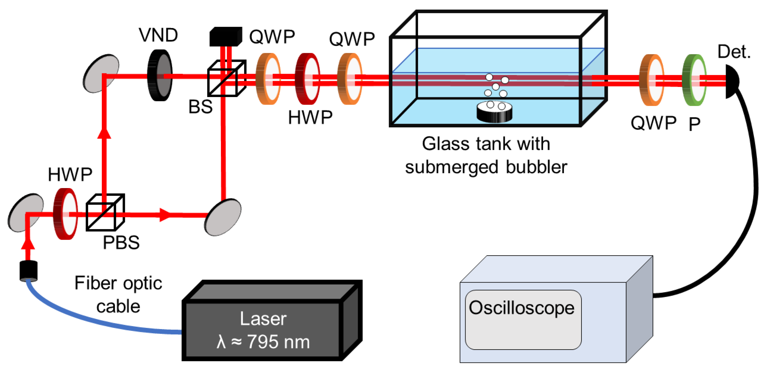
2.1. Experiment
2.2. Simulation
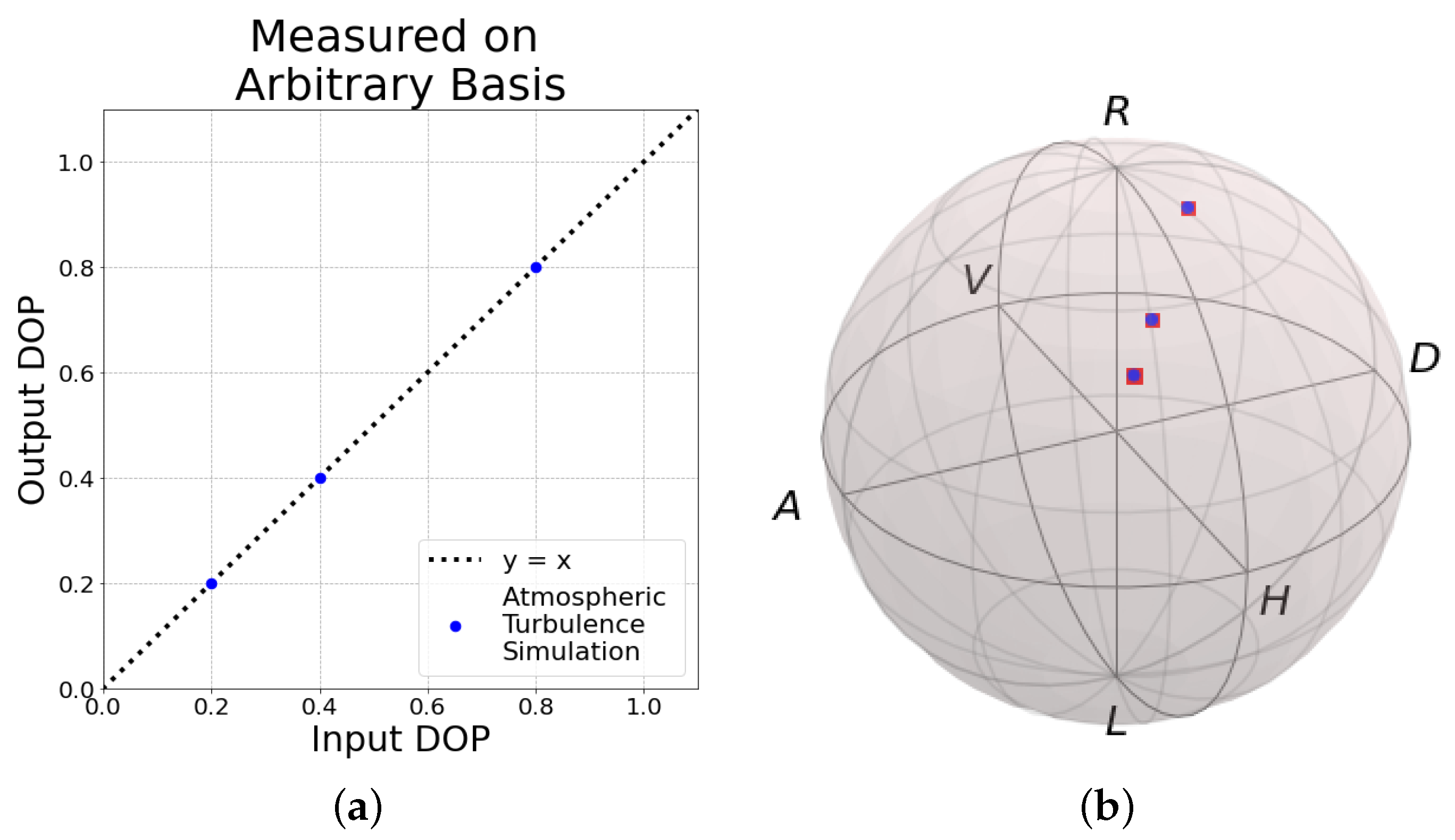
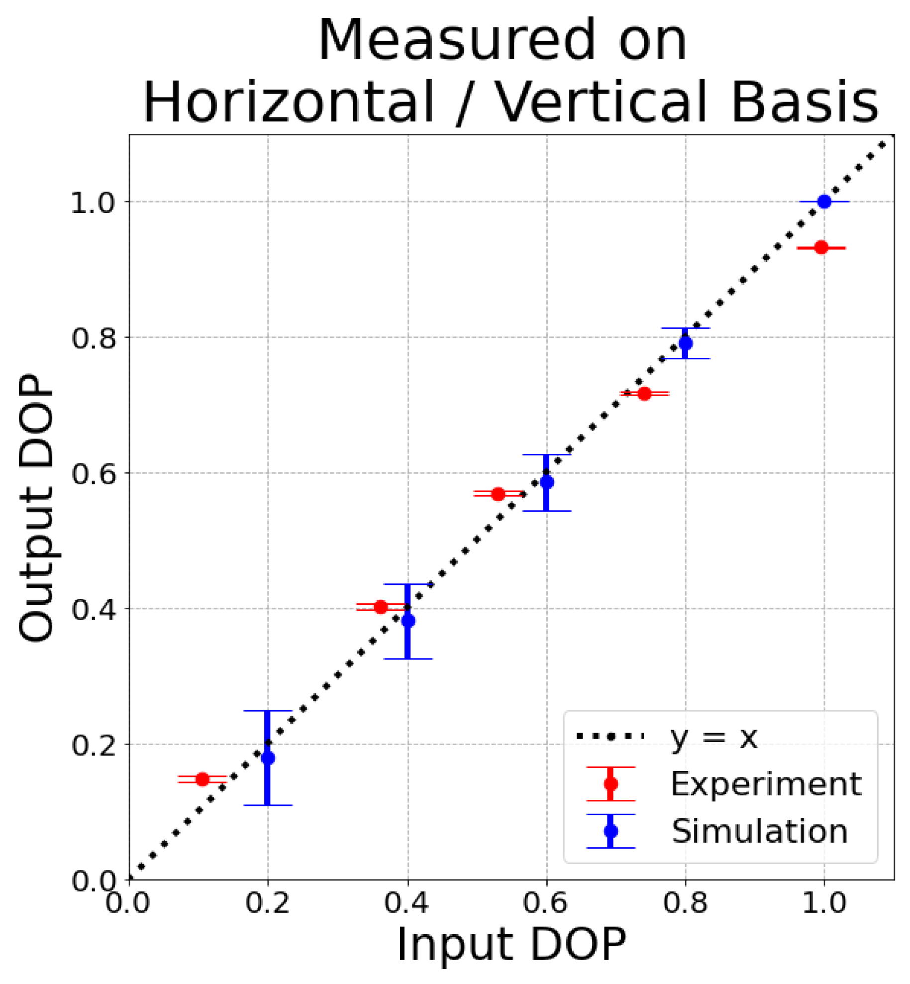
3. Results
4. Discussion
Author Contributions
Funding
Data Availability Statement
Acknowledgments
Conflicts of Interest
Abbreviations
| DOP | Degree of polarization |
| FSO | Free-space optics |
| SOP | State of polarization |
| LP | Linear polarizer |
| BS | Beam splitter |
| QWP | Quarter wave plate |
| HWP | Half wave plate |
| Det. | Detector |
| VND | Variable neutral density |
Appendix A. Simulation of Atmospheric Turbulence
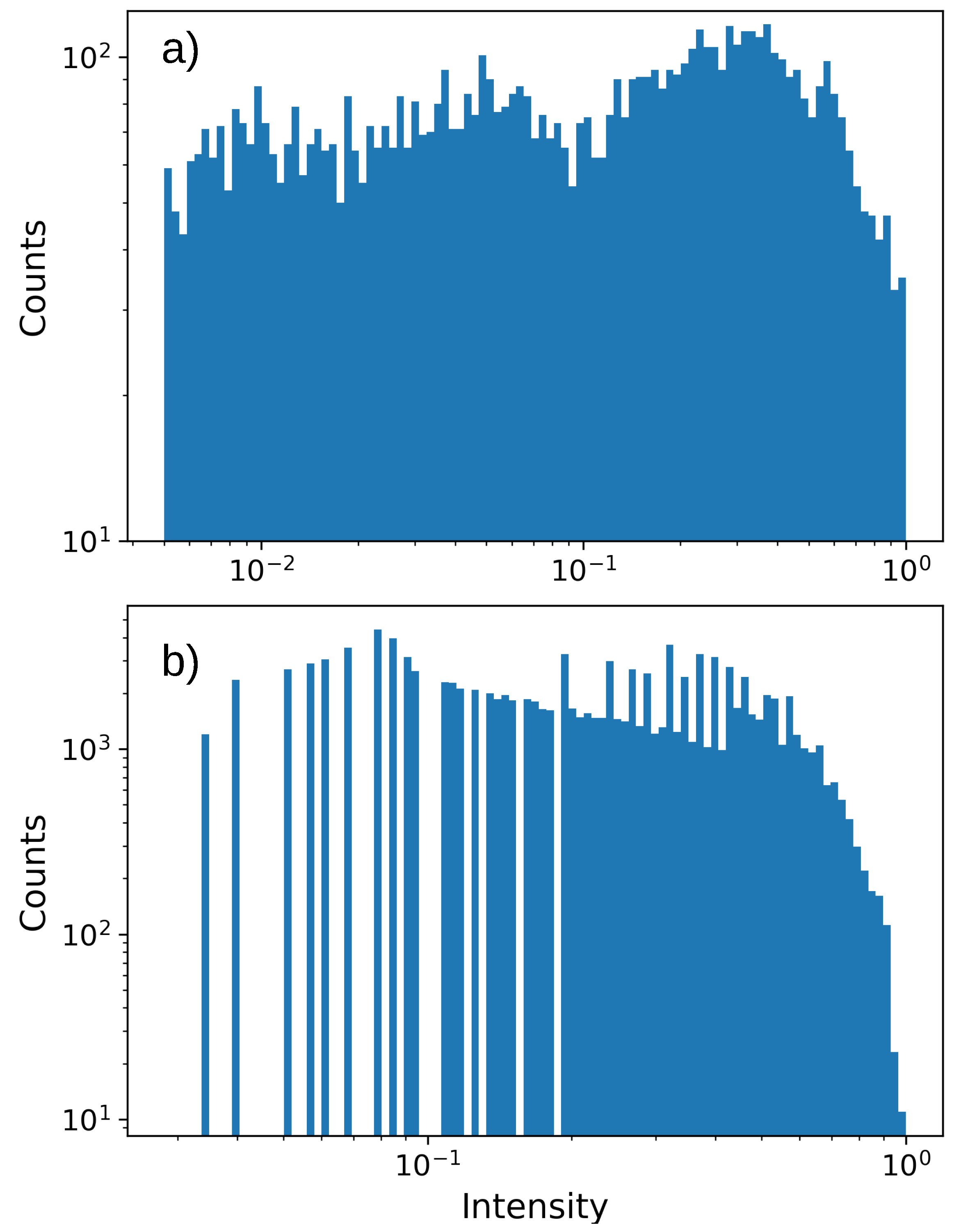
Appendix B. Intensity Distribution

References
- Malik, A.; Singh, P. Free space optics: Current applications and future challenges. Int. J. Opt. 2015, 2015, 945483. [Google Scholar] [CrossRef]
- Khalighi, M.A.; Uysal, M. Survey on Free Space Optical Communication: A Communication Theory Perspective. IEEE Commun. Surv. Tutor. 2014, 16, 2231–2258. [Google Scholar] [CrossRef]
- Willebrand, H.A.; Ghuman, B.S. Fiber optics without fiber. IEEE Spectr. 2001, 38, 40–45. [Google Scholar] [CrossRef]
- Yang, L.; Zhu, B.; Cheng, J.; Holzman, J.F. Free-Space Optical Communications Using on–off Keying and Source Information Transformation. J. Light. Technol. 2016, 34, 2601–2609. [Google Scholar] [CrossRef]
- Majumdar, A.K. Chapter 4—Fundamentals of Free-Space Optical Communications Systems, Optical Channels, Characterization, and Network/Access Technology. In Optical Wireless Communications for Broadband Global Internet Connectivity; Majumdar, A.K., Ed.; Elsevier: Amsterdam, The Netherlands, 2019; pp. 55–116. [Google Scholar] [CrossRef]
- Andrews, L.C.; Phillips, R.L.; Young, C.Y. Laser Beam Scintillation with Applications; SPIE Press: Bellingham, WA, USA, 2001. [Google Scholar] [CrossRef]
- Oh, E.S.; Ricklin, J.C.; Gilbreath, G.C.; Vallestero, N.; Eaton, F. Optical turbulence model for laser propagation and Imaging Applications. In Free-Space Laser Communication and Active Laser Illumination III; SPIE Press: Bellingham, WA, USA, 2004. [Google Scholar] [CrossRef]
- Kon, A.I.; Tatarskii, V.I. On the theory of propagation of partially coherent light beams in a turbulent atmosphere. Radiophys. Quantum Electron. 1972, 15, 1187–1192. [Google Scholar] [CrossRef]
- Trichili, A.; Ragheb, A.; Briantcev, D.; Esmail, M.A.; Altamimi, M.; Ashry, I.; Ooi, B.S.; Alshebeili, S.; Alouini, M.S. Retrofitting FSO Systems in Existing RF Infrastructure: A Non-Zero Sum Game Technology. IEEE Open J. Commun. Soc. 2021, 2, 2597–2615. [Google Scholar] [CrossRef]
- Shen, C.; Guo, Y.; Oubei, H.; Ng, T.; Liu, G.; Park, K.; Ho, K.; Alouini, M.; Ooi, B. 20-meter underwater wireless optical communication link with 1.5 Gbps data rate. Opt. Express 2016, 24, 25502–25509. [Google Scholar] [CrossRef]
- Zhu, X.; Kahn, J. Free-space optical communication through atmospheric turbulence channels. IEEE Trans. Commun. 2002, 50, 1293–1300. [Google Scholar] [CrossRef]
- Lohani, S.; Glasser, R.T. Turbulence correction with artificial neural networks. Opt. Lett. 2018, 43, 2611–2614. [Google Scholar] [CrossRef]
- Lohani, S.; Knutson, E.M.; O’Donnell, M.; Huver, S.D.; Glasser, R.T. On the use of deep neural networks in optical communications. Appl. Opt. 2018, 57, 4180–4190. [Google Scholar] [CrossRef]
- Arnon, S.; Kopeika, N. Effect of particulate on performance of optical communication in space and an adaptive method to minimize such effects. Appl. Opt. 1994, 33, 4930–4937. [Google Scholar] [CrossRef]
- Lohani, S.; Knutson, E.; Glasser, R. Generative machine learning for robust free-space communication. Commun. Phys. 2020, 3, 177. [Google Scholar] [CrossRef]
- Toyoshima, M.; Takenaka, H.; Shoji, Y.; Takayama, Y.; Koyama, Y.; Kunimori, H. Polarization measurements through space-to-ground atmospheric propagation paths by using a highly polarized laser source in space. Opt. Express 2009, 17, 22333–22340. [Google Scholar] [CrossRef]
- Peranic, M.; Clark, M.; Wang, R.; Bahrani, S.; Obada Alia, S.W.; Radman, A.; Loncaric, M.; Stipcevic, M.; Rarity, J.; Nejabati, R.; et al. A study of polarization compensation for quantum networks. EPJ Quantum Technol. 2023, 10, 30. [Google Scholar] [CrossRef]
- Goodman, J.; Skrockij, G.; Kokin, A. Statistical Optics; A Wiley-Interscience Publication; Wiley: Hoboken, NJ, USA, 1985. [Google Scholar]
- Clifford, S.F. The classical theory of wave propagation in a turbulent medium. In Laser Beam Propagation in the Atmosphere; Strohbehn, J.W., Ed.; Springer: Berlin/Heidelberg, Germany, 1978; pp. 9–43. [Google Scholar] [CrossRef]
- Strohbehn, J.; Clifford, S. Polarization and angle-of-arrival fluctuations for a plane wave propagated through a turbulent medium. IEEE Trans. Antennas Propag. 1967, 15, 416–421. [Google Scholar] [CrossRef]
- Zhang, W.; Saripalli, R.K.; Leamer, J.M.; Glasser, R.T.; Bondar, D.I. All-optical input-agnostic polarization transformer. arXiv 2021, arXiv:2103.05398. [Google Scholar]
- Cvijetic, N.; Qian, D.; Yu, J.; Huang, Y.K.; Wang, T. Polarization-Multiplexed Optical Wireless Transmission with Coherent Detection. J. Light. Technol. 2010, 28, 1218–1227. [Google Scholar] [CrossRef]
- Rosskopf, M.; Mohr, T.; Elsäßer, W. Ghost Polarization Communication. Phys. Rev. Appl. 2020, 13, 034062. [Google Scholar] [CrossRef]
- Zhang, J.; Li, R.; Dang, A. Experimental Studies on Characteristics of Polarization Parameters over Atmospheric Turbulence. In Proceedings of the ECOC 2016—42nd European Conference on Optical Communication, Dusseldorf, Germany, 18–22 September 2016; pp. 1–3. [Google Scholar]
- Tang, X.; Xu, Z.; Ghassemlooy, Z. Coherent Polarization Modulated Transmission through MIMO Atmospheric Optical Turbulence Channel. J. Light. Technol. 2013, 31, 3221–3228. [Google Scholar] [CrossRef]
- Yang, R.; Xue, Y.; Li, Y.; Shi, L.; Zhu, Y.; Zhu, Q. Influence of atmospheric turbulence on the quantum polarization state. In Young Scientists Forum 2017; Zhuang, S., Chu, J., Pan, J.W., Eds.; International Society for Optics and Photonics, SPIE: Bellingham, WA, USA, 2018; Volume 10710, pp. 36–41. [Google Scholar] [CrossRef]
- Sait, M.; Sun, X.; Alkhazragi, O.; Alfaraj, N.; Kong, M.; Ng, T.K.; Ooi, B.S. The effect of turbulence on NLOS underwater wireless optical communication channels [Invited]. Chin. Opt. Lett. 2019, 17, 100013. [Google Scholar] [CrossRef]
- Zedini, E.; Oubei, H.M.; Kammoun, A.; Hamdi, M.; Ooi, B.S.; Alouini, M.S. Unified Statistical Channel Model for Turbulence-Induced Fading in Underwater Wireless Optical Communication Systems. IEEE Trans. Commun. 2019, 67, 2893–2907. [Google Scholar] [CrossRef]
- Jamali, M.V.; Mirani, A.; Parsay, A.; Abolhassani, B.; Nabavi, P.; Chizari, A.; Khorramshahi, P.; Abdollahramezani, S.; Salehi, J.A. Statistical Studies of Fading in Underwater Wireless Optical Channels in the Presence of Air Bubble, Temperature, and Salinity Random Variations. IEEE Trans. Commun. 2018, 66, 4706–4723. [Google Scholar] [CrossRef]
- Oubei, H.M.; ElAfandy, R.T.; Park, K.H.; Ng, T.K.; Alouini, M.S.; Ooi, B.S. Performance Evaluation of Underwater Wireless Optical Communications Links in the Presence of Different Air Bubble Populations. IEEE Photonics J. 2017, 9, 7903009. [Google Scholar] [CrossRef]
- Shin, M.; Park, K.H.; Alouini, M.S. Statistical Modeling of the Impact of Underwater Bubbles on an Optical Wireless Channel. IEEE Open J. Commun. Soc. 2020, 1, 808–818. [Google Scholar] [CrossRef]
- Barberena, D.; Gatti, G.; Zela, F.D. Experimental demonstration of a secondary source of partially polarized states. J. Opt. Soc. Am. A 2015, 32, 697–700. [Google Scholar] [CrossRef] [PubMed]
- Ijaz, M. Experimental Characterisation and Modelling of Atmospheric Fog and Turbulence in FSO. Ph.D. Thesis, Northumbria University, Newcastle upon Tyne, UK, 2013. [Google Scholar]
- van Vliet, V.; van der Heide, S.; van den Hout, M.; Okonkwo, C. Turbulence Characterisation for Free Space Optical Communication Using Off-Axis Digital Holography. In Signal Processing in Photonic Communications; Optica Publishing Group: Washington, DC, USA, 2022. [Google Scholar] [CrossRef]
- Leamer, J.M.; Zhang, W.; Saripalli, R.K.; Glasser, R.T.; Bondar, D.I. Robust polarimetry via convex optimization. Appl. Opt. 2020, 59, 8886–8894. [Google Scholar] [CrossRef] [PubMed]
- Schaefer, B.; Collett, E.; Smyth, R.; Barrett, D.; Fraher, B. Measuring the Stokes polarization parameters. Am. J. Phys. 2007, 75, 163–168. [Google Scholar] [CrossRef]
- COMSOL Multiphysics ®v. 6.0; COMSOL AB: Stockholm, Sweden; Available online: https://www.comsol.com/release/6.0 (accessed on 26 March 2024).
- Leamer, J.M. DOP Communication. 2020. Available online: https://github.com/jleamer/DOP_Comm (accessed on 26 March 2024).
- Son, I.K.; Mao, S. A survey of free space optical networks. Digit. Commun. Netw. 2017, 3, 67–77. [Google Scholar] [CrossRef]
- Kaushal, H.; Kaddoum, G. Underwater Optical Wireless Communication. IEEE Access 2016, 4, 1518–1547. [Google Scholar] [CrossRef]
- Bennett, C.H.; Brassard, G. Quantum cryptography: Public key distribution and coin tossing. Proc. IEEE Int. Conf. Comput. Syst. Signal Process. 1984, 175, 8. [Google Scholar] [CrossRef]
- Wu, H.W.; Lu, H.H.; Tsai, W.S.; Huang, Y.C.; Xie, J.Y.; Huang, Q.P.; Tu, S.C. A 448-Gb/s PAM4 FSO Communication with Polarization-Multiplexing Injection-Locked VCSELs through 600 M Free-Space Link. IEEE Access 2020, 8, 28859–28866. [Google Scholar] [CrossRef]
- Willner, A.; Ren, Y.; Xie, G.; Yan, Y.; Li, L.; Zhao, Z.; Wang, J.; Tur, M.; Molisch, A.; Ashrafi, S. Recent advances in high-capacity free-space optical and radio-frequency communications using orbital angular momentum multiplexing. Philos. Trans. R. Soc. Math. Phys. Eng. Sci. 2017, 375, 20150439. [Google Scholar] [CrossRef] [PubMed]
- Takenaka, H.; Carrasco-Casado, A.; Fujiwara, M.; Kitamura, M.; Sasaki, M.; Toyoshima, M. Satellite-to-ground quantum-limited communication using a 50-kg-class microsatellite. Nat. Photonics 2017, 11, 502–508. [Google Scholar] [CrossRef]
- Zhang, D.; Hao, S.; Zhao, Q.; Zhang, M.; Fan, B. Atmospheric turbulence phase screen modeling method based on sub-bands division and multirate sampling. Optik 2018, 163, 72–80. [Google Scholar] [CrossRef]
- Martin, J.M.; Flatté, S.M. Intensity images and statistics from numerical simulation of wave propagation in 3-D random media. Appl. Opt. 1988, 27, 2111–2126. [Google Scholar] [CrossRef] [PubMed]
- Rampy, R.; Gavel, D.; Dillon, D.; Thomas, S. Production of phase screens for simulation of atmospheric turbulence. Appl. Opt. 2012, 51, 8769–8778. [Google Scholar] [CrossRef] [PubMed]
- Wild, A.J.; Hobbs, R.W.; Frenje, L. Modelling complex media: An introduction to the phase-screen method. Phys. Earth Planet. Inter. 2000, 120, 219–225. [Google Scholar] [CrossRef]
- Wu, R.S. Wide-angle elastic wave one-way propagation in heterogeneous media and an elastic wave complex-screen method. J. Geophys. Res. Solid Earth 1994, 99, 751–766. [Google Scholar] [CrossRef]
- Vorontsov, A.M.; Paramonov, P.V.; Valley, M.T.; Vorontsov, M.A. Generation of infinitely long phase screens for modeling of optical wave propagation in atmospheric turbulence. Waves Random Complex Media 2008, 18, 91–108. [Google Scholar] [CrossRef]
- Buckley, R. Diffraction by a random phase-changing screen: A numerical experiment. J. Atmos. Terr. Phys. 1975, 37, 1431–1446. [Google Scholar] [CrossRef]


| Parameter | Symbol | Value |
|---|---|---|
| Power transmitted | ≈24 dBm | |
| Transmitter gain | ≈0 dB | |
| Transmitter loss | ≈15 to 18 dB | |
| Free-space loss | ≈0 dB | |
| Turbulence related loss | ≈13 dB | |
| Receiver gain | ≈0 dB | |
| Receiver loss | ≈0 to 20 dB |
| State | DOP | |||||||
|---|---|---|---|---|---|---|---|---|
| Input | Output | Input | Output | Input | Output | Input | Output | |
| 0 | 0.09 | 0.14 | −0.04 | 0.01 | −0.04 | −0.05 | 0.11 | 0.15 |
| 1 | 0.36 | 0.39 | −0.05 | −0.07 | −0.03 | −0.07 | 0.36 | 0.40 |
| 2 | 0.53 | 0.55 | −0.04 | −0.08 | −0.02 | −0.10 | 0.53 | 0.57 |
| 3 | 0.74 | 0.71 | −0.05 | −0.03 | −0.02 | −0.06 | 0.74 | 0.72 |
| 4 | 0.99 | 0.92 | −0.06 | −0.10 | −0.02 | −0.08 | 0.99 | 0.93 |
| State | DOP | |||||||
|---|---|---|---|---|---|---|---|---|
| Input | Output | Input | Output | Input | Output | Input | Output | |
| 0 | 0.03 | 0.04 | 0.06 | −0.02 | 0.05 | 0.10 | 0.08 | 0.11 |
| 1 | 0.08 | 0.11 | −0.11 | −0.15 | 0.29 | 0.33 | 0.32 | 0.38 |
| 2 | 0.12 | 0.13 | −0.32 | −0.25 | 0.43 | 0.43 | 0.55 | 0.51 |
| 3 | 0.18 | 0.17 | −0.45 | −0.36 | 0.62 | 0.68 | 0.79 | 0.79 |
| 4 | 0.25 | 0.25 | −0.43 | −0.47 | 0.78 | 0.73 | 0.93 | 0.91 |
Disclaimer/Publisher’s Note: The statements, opinions and data contained in all publications are solely those of the individual author(s) and contributor(s) and not of MDPI and/or the editor(s). MDPI and/or the editor(s) disclaim responsibility for any injury to people or property resulting from any ideas, methods, instructions or products referred to in the content. |
© 2024 by the authors. Licensee MDPI, Basel, Switzerland. This article is an open access article distributed under the terms and conditions of the Creative Commons Attribution (CC BY) license (https://creativecommons.org/licenses/by/4.0/).
Share and Cite
Savino, N.; Leamer, J.; Saripalli, R.; Zhang, W.; Bondar, D.; Glasser, R. Robust Free-Space Optical Communication Utilizing Polarization for the Advancement of Quantum Communication. Entropy 2024, 26, 309. https://doi.org/10.3390/e26040309
Savino N, Leamer J, Saripalli R, Zhang W, Bondar D, Glasser R. Robust Free-Space Optical Communication Utilizing Polarization for the Advancement of Quantum Communication. Entropy. 2024; 26(4):309. https://doi.org/10.3390/e26040309
Chicago/Turabian StyleSavino, Nicholas, Jacob Leamer, Ravi Saripalli, Wenlei Zhang, Denys Bondar, and Ryan Glasser. 2024. "Robust Free-Space Optical Communication Utilizing Polarization for the Advancement of Quantum Communication" Entropy 26, no. 4: 309. https://doi.org/10.3390/e26040309
APA StyleSavino, N., Leamer, J., Saripalli, R., Zhang, W., Bondar, D., & Glasser, R. (2024). Robust Free-Space Optical Communication Utilizing Polarization for the Advancement of Quantum Communication. Entropy, 26(4), 309. https://doi.org/10.3390/e26040309