
Fractal Conditional Correlation Dimension Infers Complex Causal Networks


Abstract
1. Introduction
2. Problem Statement
2.1. Preliminaries and Basic Definitions
2.2. Geometric Causation of Information Flow in Networks
| Algorithm 1 Algorithm |
|
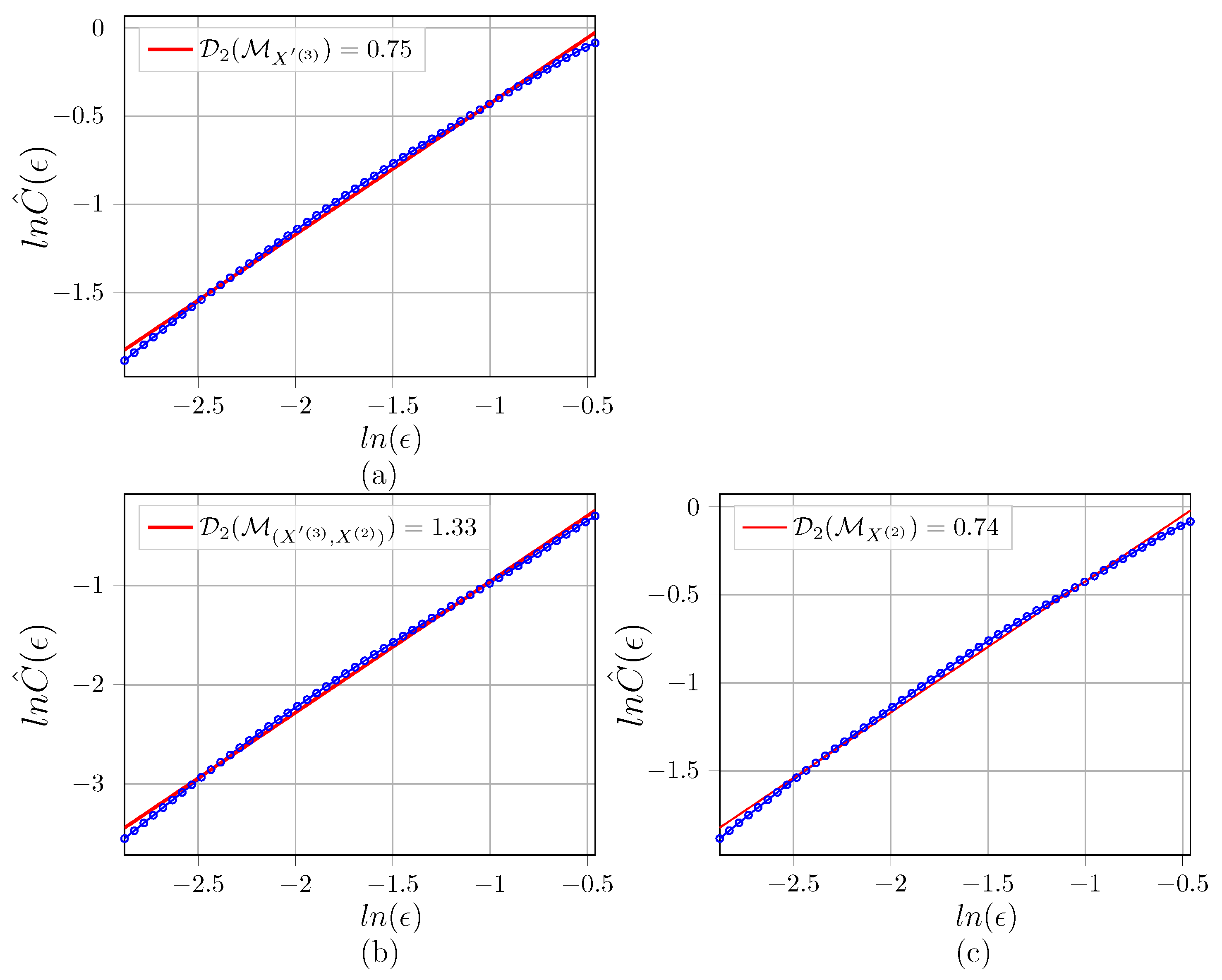
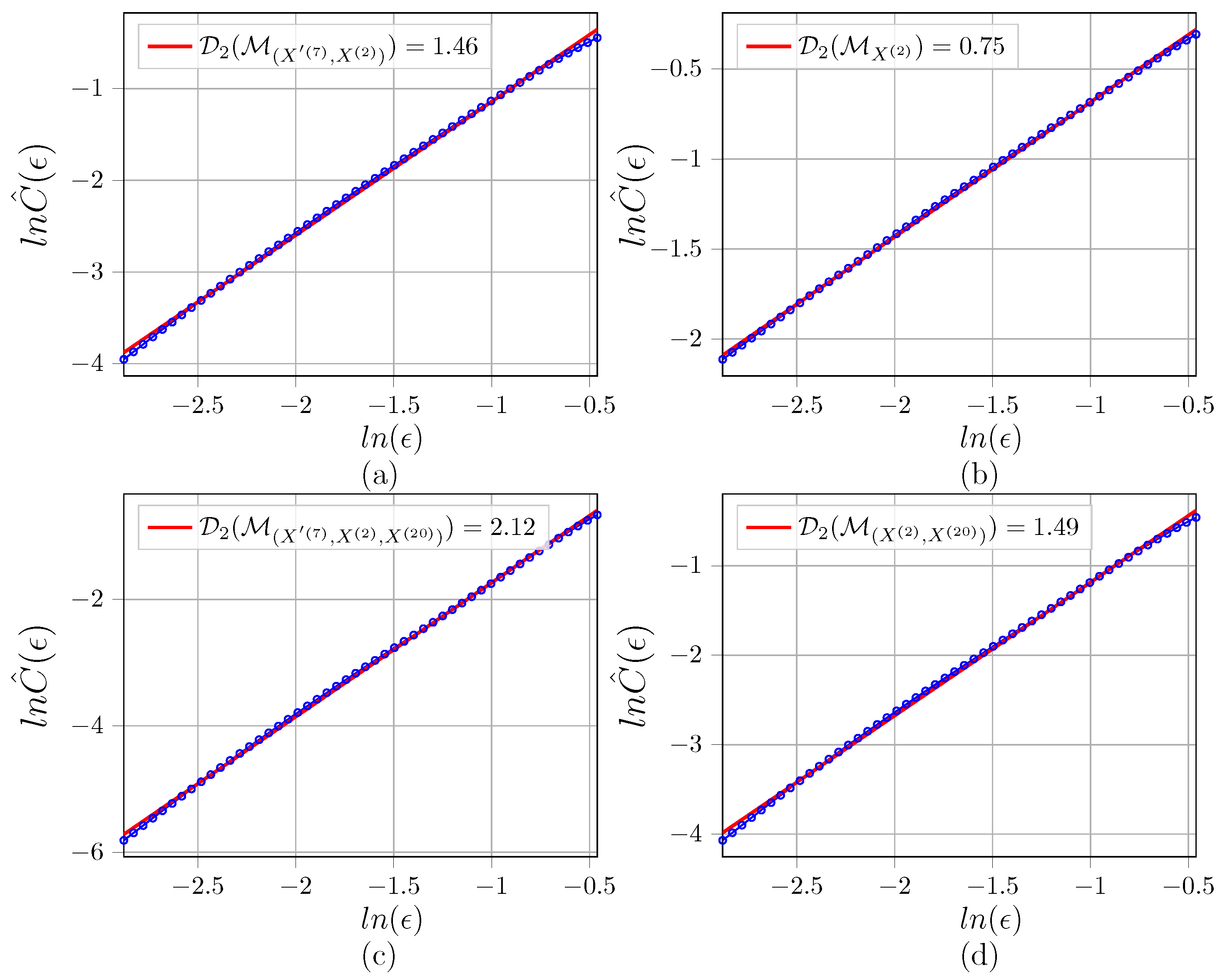
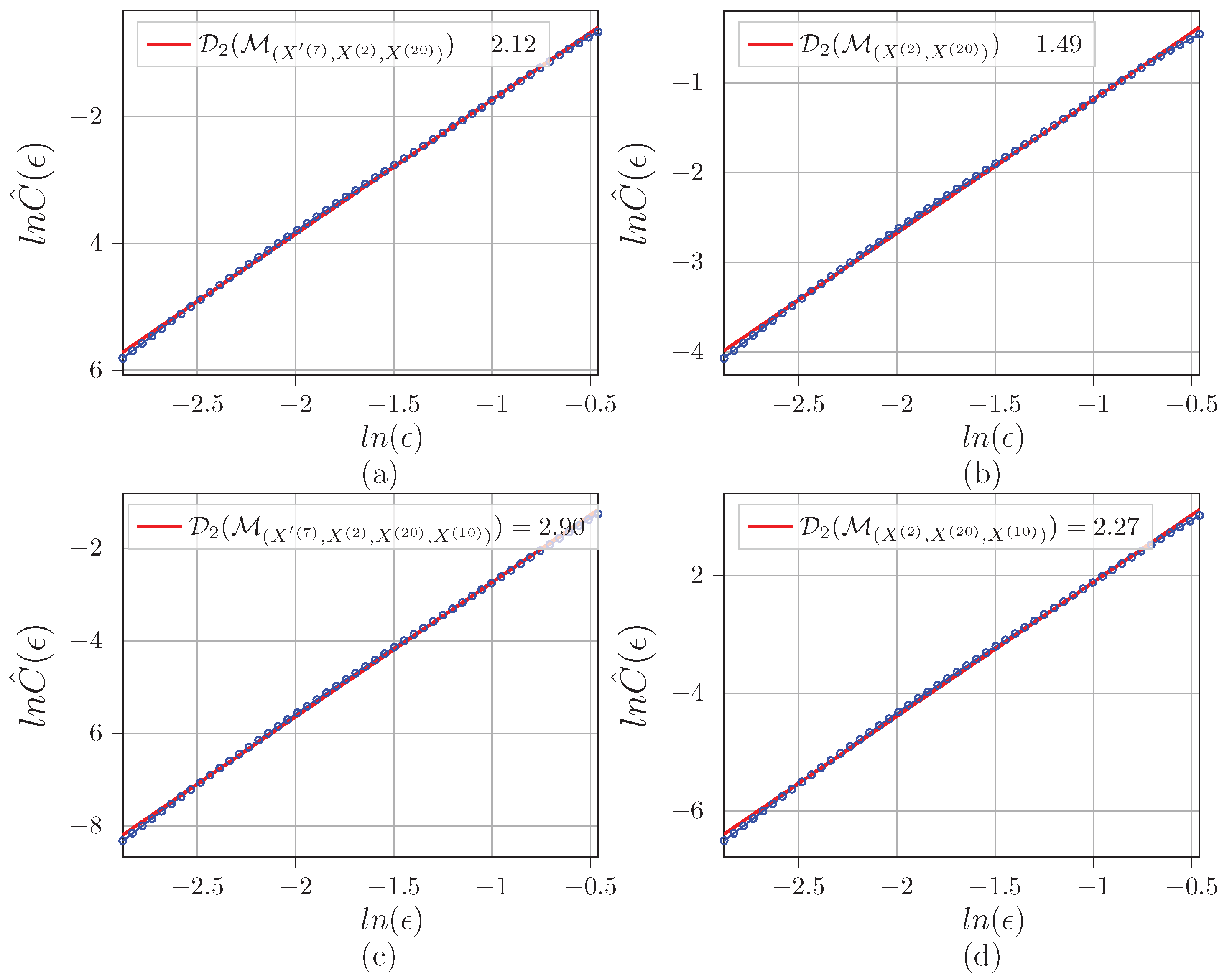
Estimation of Correlation Dimension
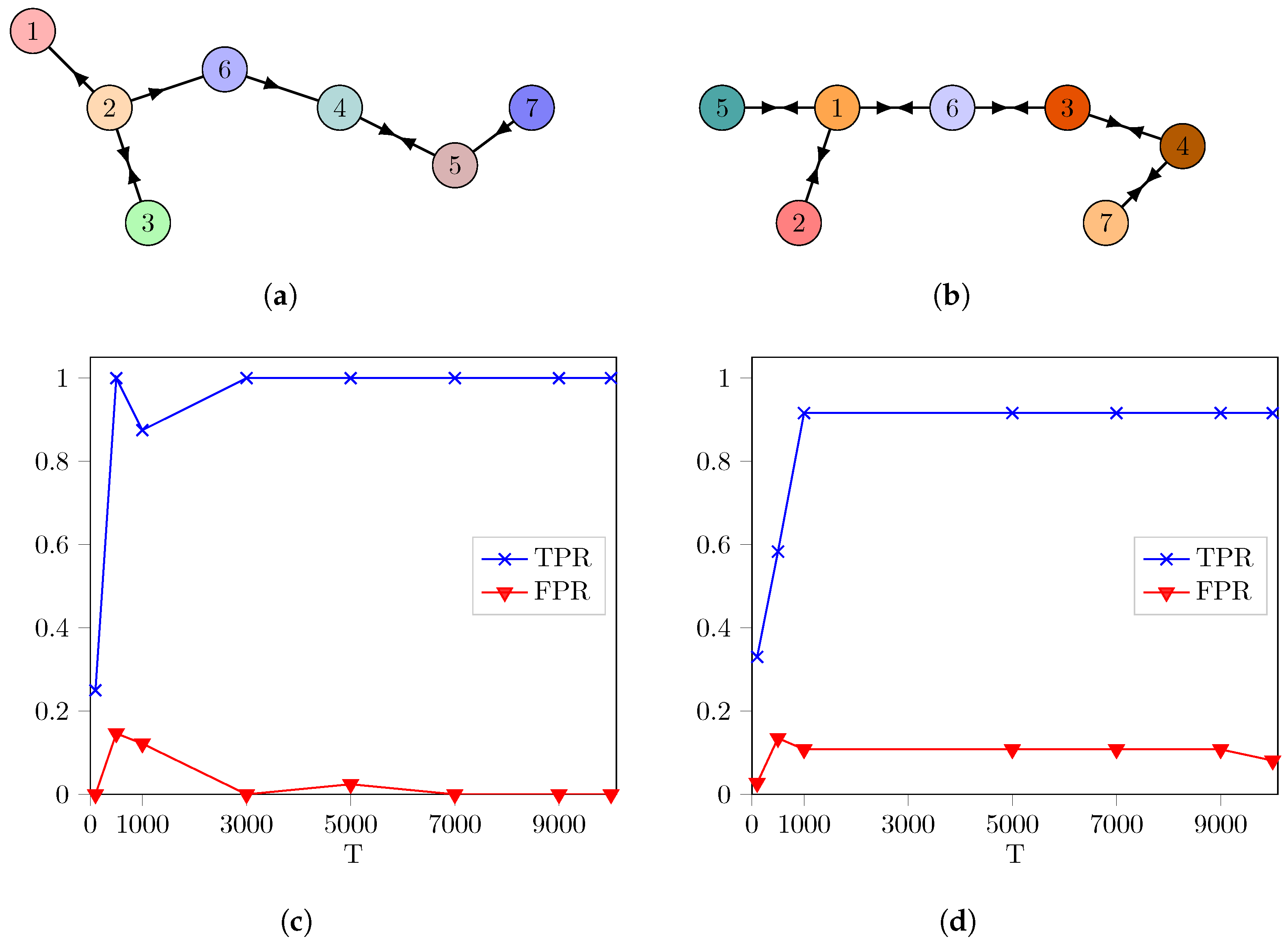
3. Results
4. Discussion
Author Contributions
Funding
Institutional Review Board Statement
Data Availability Statement
Acknowledgments
Conflicts of Interest
Appendix A. Estimation of Correlation Dimension
| Algorithm A1 Estimation |
|
Appendix B. Shuffle Test to Determine the Zero
| Algorithm A2 Shuffle Test |
|
Appendix C. Illustration of D 2 Estimations for the Networks


References
- Sudu Ambegedara, A.; Sun, J.; Janoyan, K.; Bollt, E. Information-theoretical noninvasive damage detection in bridge structures. arXiv 2016, arXiv:1612.09340. [Google Scholar] [CrossRef] [PubMed]
- Runge, J.; Bathiany, S.; Bollt, E.; Camps-Valls, G.; Coumou, D.; Deyle, E.; Glymour, C.; Kretschmer, M.; Mahecha, M.D.; Muñoz-Marí, J.; et al. Inferring causation from time series in Earth system sciences. Nat. Commun. 2019, 10, 2553. [Google Scholar] [CrossRef] [PubMed]
- Runge, J.; Gerhardus, A.; Varando, G.; Eyring, V.; Camps-Valls, G. Causal inference for time series. Nat. Rev. Earth Environ. 2023, 4, 487–505. [Google Scholar] [CrossRef]
- Seth, A.K.; Chorley, P.; Barnett, L.C. Granger causality analysis of fMRI BOLD signals is invariant to hemodynamic convolution but not downsampling. Neuroimage 2013, 65, 540–555. [Google Scholar] [CrossRef] [PubMed]
- Sugihara, G.; May, R.; Ye, H.; Hsieh, C.h.; Deyle, E.; Fogarty, M.; Munch, S. Detecting causality in complex ecosystems. Science 2012, 338, 496–500. [Google Scholar] [CrossRef]
- Bollt, E.M. Open or closed? Information flow decided by transfer operators and forecastability quality metric. arXiv 2018, arXiv:1804.03687. [Google Scholar] [CrossRef]
- Surasinghe, S.; Bollt, E.M. On geometry of information flow for causal inference. Entropy 2020, 22, 396. [Google Scholar] [CrossRef]
- Hendry, D.F. The nobel memorial prize for clive wj granger. Scand. J. Econ. 2004, 106, 187–213. [Google Scholar] [CrossRef]
- Wiener, N. The theory of prediction. In Modern Mathematics for Engineers; McGraw Hill: New York, NY, USA, 1956. [Google Scholar]
- Granger, C.W. Investigating causal relations by econometric models and cross-spectral methods. Econometrica 1969, 424–438. [Google Scholar] [CrossRef]
- Marinazzo, D.; Pellicoro, M.; Stramaglia, S. Kernel method for nonlinear Granger causality. Phys. Rev. Lett. 2008, 100, 144103. [Google Scholar] [CrossRef] [PubMed]
- Barrett, A.B.; Barnett, L.; Seth, A.K. Multivariate Granger causality and generalized variance. Phys. Rev. E 2010, 81, 041907. [Google Scholar] [CrossRef] [PubMed]
- Marinazzo, D.; Liao, W.; Chen, H.; Stramaglia, S. Nonlinear connectivity by Granger causality. Neuroimage 2011, 58, 330–338. [Google Scholar] [CrossRef] [PubMed]
- Rulkov, N.F.; Sushchik, M.M.; Tsimring, L.S.; Abarbanel, H.D. Generalized synchronization of chaos in directionally coupled chaotic systems. Phys. Rev. E 1995, 51, 980. [Google Scholar] [CrossRef] [PubMed]
- Schiff, S.J.; So, P.; Chang, T.; Burke, R.E.; Sauer, T. Detecting dynamical interdependence and generalized synchrony through mutual prediction in a neural ensemble. Phys. Rev. E 1996, 54, 6708. [Google Scholar] [CrossRef] [PubMed]
- Arnhold, J.; Grassberger, P.; Lehnertz, K.; Elger, C.E. A robust method for detecting interdependences: Application to intracranially recorded EEG. Phys. D Nonlinear Phenom. 1999, 134, 419–430. [Google Scholar] [CrossRef]
- Quiroga, R.Q.; Kraskov, A.; Kreuz, T.; Grassberger, P. Performance of different synchronization measures in real data: A case study on electroencephalographic signals. Phys. Rev. E 2002, 65, 041903. [Google Scholar] [CrossRef]
- Andrzejak, R.G.; Kraskov, A.; Stögbauer, H.; Mormann, F.; Kreuz, T. Bivariate surrogate techniques: Necessity, strengths, and caveats. Phys. Rev. E 2003, 68, 066202. [Google Scholar] [CrossRef]
- Chicharro, D.; Andrzejak, R.G. Reliable detection of directional couplings using rank statistics. Phys. Rev. E 2009, 80, 026217. [Google Scholar] [CrossRef]
- Ye, H.; Deyle, E.R.; Gilarranz, L.J.; Sugihara, G. Distinguishing time-delayed causal interactions using convergent cross mapping. Sci. Rep. 2015, 5, 14750. [Google Scholar] [CrossRef]
- Mønster, D.; Fusaroli, R.; Tylén, K.; Roepstorff, A.; Sherson, J.F. Causal inference from noisy time-series data—Testing the Convergent Cross-Mapping algorithm in the presence of noise and external influence. Future Gener. Comput. Syst. 2017, 73, 52–62. [Google Scholar] [CrossRef]
- Breston, L.; Leonardis, E.J.; Quinn, L.K.; Tolston, M.; Wiles, J.; Chiba, A.A. Convergent cross sorting for estimating dynamic coupling. Sci. Rep. 2021, 11, 20374. [Google Scholar] [CrossRef] [PubMed]
- Schreiber, T. Measuring information transfer. Phys. Rev. Lett. 2000, 85, 461. [Google Scholar] [CrossRef] [PubMed]
- Sun, J.; Bollt, E.M. Causation entropy identifies indirect influences, dominance of neighbors and anticipatory couplings. Phys. D Nonlinear Phenom. 2014, 267, 49–57. [Google Scholar] [CrossRef]
- Sun, J.; Taylor, D.; Bollt, E.M. Causal network inference by optimal causation entropy. SIAM J. Appl. Dyn. Syst. 2015, 14, 73–106. [Google Scholar] [CrossRef]
- Lord, W.M.; Sun, J.; Ouellette, N.T.; Bollt, E.M. Inference of causal information flow in collective animal behavior. IEEE Trans. Mol. Biol. Multi-Scale Commun. 2016, 2, 107–116. [Google Scholar] [CrossRef]
- Janjarasjitt, S.; Loparo, K. An approach for characterizing coupling in dynamical systems. Phys. D Nonlinear Phenom. 2008, 237, 2482–2486. [Google Scholar] [CrossRef]
- Krakovská, A.; Budáčová, H. Interdependence measure based on correlation dimension. In Proceedings of the 9th International Conference on Measurement, Bratislava, Slovakia, 27–30 May 2013; pp. 31–34. [Google Scholar]
- Krakovská, A.; Jakubík, J.; Budáčová, H.; Holecyová, M. Causality studied in reconstructed state space. Examples of uni-directionally connected chaotic systems. arXiv 2015, arXiv:1511.00505. [Google Scholar]
- Krakovská, A. Correlation dimension detects causal links in coupled dynamical systems. Entropy 2019, 21, 818. [Google Scholar] [CrossRef]
- Takens, F. Detecting strange attractors in turbulence. In Dynamical Systems and Turbulence; Springer: New York, NY, USA, 1981; pp. 366–381. [Google Scholar]
- Cummins, B.; Gedeon, T.; Spendlove, K. On the efficacy of state space reconstruction methods in determining causality. SIAM J. Appl. Dyn. Syst. 2015, 14, 335–381. [Google Scholar] [CrossRef]
- Kantz, H.; Schreiber, T. Nonlinear Time Series Analysis; Cambridge University Press: Cambridge, UK, 2003. [Google Scholar]
- Sauer, T.; Yorke, J.A.; Casdagli, M. Embedology. J. Stat. Phys. 1991, 65, 579–616. [Google Scholar] [CrossRef]
- Good, P. Permutation, Parametric, and Bootstrap Tests of Hypotheses; Springer: New York, NY, USA, 2005. [Google Scholar]
- Grassberger, P.; Procaccia, I. Characterization of strange attractors. Phys. Rev. Lett. 1983, 50, 346. [Google Scholar] [CrossRef]
- Grassberger, P.; Procaccia, I. Measuring the strangeness of strange attractors. Phys. D Nonlinear Phenom. 1983, 9, 189–208. [Google Scholar] [CrossRef]
- Theiler, J. Efficient algorithm for estimating the correlation dimension from a set of discrete points. Phys. Rev. A 1987, 36, 4456. [Google Scholar] [CrossRef] [PubMed]
- Abarbanel, H. Analysis of Observed Chaotic Data; Springer Science & Business Media: New York, NY, USA, 2012. [Google Scholar]
- Sammut, C.; Webb, G.I. Encyclopedia of Machine Learning; Springer Science & Business Media: New York, NY, USA, 2011. [Google Scholar]
- Erdős, P.; Rényi, A. On the evolution of random graphs. Publ. Math. Inst. Hung. Acad. Sci. 1960, 5, 17–60. [Google Scholar]
- Eckmann, J.P.; Ruelle, D. Fundamental limitations for estimating dimensions and Lyapunov exponents in dynamical systems. Phys. D Nonlinear Phenom. 1992, 56, 185–187. [Google Scholar] [CrossRef]
- Schreiber, T. Determination of the noise level of chaotic time series. Phys. Rev. E 1993, 48, R13. [Google Scholar] [CrossRef]
- Ji, C.; Zhu, H.; Jiang, W. A novel method to identify the scaling region for chaotic time series correlation dimension calculation. Chi. Sci. Bull. 2011, 56, 925–932. [Google Scholar] [CrossRef]
- Krakovská, A.; Chvosteková, M. Simple correlation dimension estimator and its use to detect causality. Chaos Solitons Fractals 2023, 175, 113975. [Google Scholar] [CrossRef]
- Makarov, V.A.; Muñoz, R.; Herreras, O.; Makarova, J. Correlation dimension of high-dimensional and high-definition experimental time series. Chaos Interdiscip. Nonlinear Sci. 2023, 33, 123114. [Google Scholar] [CrossRef]
- Porta, A.; de Abreu, R.M.; Bari, V.; Gelpi, F.; De Maria, B.; Catai, A.M.; Cairo, B. On the validity of the state space correspondence strategy based on k-nearest neighbor cross-predictability in assessing directionality in stochastic systems: Application to cardiorespiratory coupling estimation. Chaos An Interdiscip. J. Nonlinear Sci. 2024, 34, 053115. [Google Scholar] [CrossRef]
Disclaimer/Publisher’s Note: The statements, opinions and data contained in all publications are solely those of the individual author(s) and contributor(s) and not of MDPI and/or the editor(s). MDPI and/or the editor(s) disclaim responsibility for any injury to people or property resulting from any ideas, methods, instructions or products referred to in the content. |
© 2024 by the authors. Licensee MDPI, Basel, Switzerland. This article is an open access article distributed under the terms and conditions of the Creative Commons Attribution (CC BY) license (https://creativecommons.org/licenses/by/4.0/).
Share and Cite
Canlı Usta, Ö.; Bollt, E.M. Fractal Conditional Correlation Dimension Infers Complex Causal Networks. Entropy 2024, 26, 1030. https://doi.org/10.3390/e26121030
Canlı Usta Ö, Bollt EM. Fractal Conditional Correlation Dimension Infers Complex Causal Networks. Entropy. 2024; 26(12):1030. https://doi.org/10.3390/e26121030
Chicago/Turabian StyleCanlı Usta, Özge, and Erik M. Bollt. 2024. "Fractal Conditional Correlation Dimension Infers Complex Causal Networks" Entropy 26, no. 12: 1030. https://doi.org/10.3390/e26121030
APA StyleCanlı Usta, Ö., & Bollt, E. M. (2024). Fractal Conditional Correlation Dimension Infers Complex Causal Networks. Entropy, 26(12), 1030. https://doi.org/10.3390/e26121030