1. Introduction
Integer-valued time series are ubiquitous in scientific research and everyday life, encompassing examples such as the daily count of hospitalized patients admitted to hospitals and the frequency of crimes committed daily or monthly. Consequently, integer-valued time series have increasingly garnered attention from scholars. However, traditional continuous-valued time series models fail to capture the integer-valued characteristics, only approximating integer-valued data through continuous-valued time series models. This approximation may result in model misspecification issues, complicating statistical inference. As a result, the modeling and analysis of integer-valued time series data have become a growing area of focus in academia. Among the variety of integer-valued time series modeling methods, thinning operator models have gained favor due to their resemblance to autoregressive moving average (ARMA) models found in traditional continuous-valued time series theory. Thinning operator models substitute the multiplication in ARMA models with the binomial thinning operator introduced by Steutel and Van Harn [
1]:
In this equation,
represents a count sequence, while
denotes a series of Bernoulli random variables independent of
. The probability mass function satisfies
with
. Building on this foundation, Al-Osh and Alzaid [
2] developed the first-order integer-valued autoregressive (INAR (1)) model for
:
where
is regarded as the innovation term entering the model at period
, with its marginal distribution being a Poisson distribution with an expected value of
. Consequently, model (2) is called the Poisson INAR(1) model. Later, Du and Li [
3] introduced the INAR(p) model and provided conditions for ensuring the stationarity and ergodicity of the INAR(p) process. The incorporation of additional lag terms increased the model’s flexibility. Subsequently, Joe [
4] and Zheng, Basawa, and Datta [
5] developed the random coefficient thinning operator model (RCINAR(1)) by allowing the parameter
in the INAR(1) model to follow a specific random distribution. Zheng, Basawa, and Datta [
6] extended the RCINAR(1) model to the p-th order integer-valued autoregressive model, known as the RCINAR(p) model. Zhang, Wang, and Zhu [
7] established a data-driven empirical likelihood interval estimation for the RCINAR(p) model using the empirical likelihood (EL) estimation method. By employing the geometric thinning operator (also referred to as the negative binomial thinning operator) proposed by Ristić, Bakouch, and Nastić [
8], Tian, Wang, and Cui [
9]) constructed an INAR(1) model capable of describing seasonal effects. Lu [
10] investigated the prediction problem of the thinning operator model using the Taylor expansion. For further discussions on thinning operator models, readers can consult the textbook by Weiß [
11].
In general, researchers engaged in statistical analysis, particularly during the initial stages of time series data investigation, frequently encounter the challenge of model selection. Current model selection techniques can be broadly categorized into three groups: The first group relies on sample autocorrelation (ACF) and partial autocorrelation (PACF) functions for model selection, as exemplified by Latour [
12]; the second group, which is the most prevalent method for variable selection, comprises a series of information criteria founded on maximum likelihood estimation. Akaike [
13] introduced the Akaike Information Criterion (AIC) by performing an unbiased estimation of the expected log-likelihood function, while Schwarz [
14] established the Bayesian Information Criterion (BIC) by employing a Laplace expansion for the posterior estimation of the expected log-likelihood function. Ding, Tarokh, and Yang [
15] devised a novel information criterion for autoregressive time series models by connecting AIC and BIC. Furthermore, given that empirical likelihood estimation can substantially circumvent issues stemming from model misspecification and maintain certain maximum likelihood estimation features, researchers have started to investigate data-driven information criteria based on empirical likelihood estimation. Variyath, Chen, and Abraham [
16] formulated the Empirical Akaike Information Criterion (EAIC) and the Empirical Bayesian Information Criterion (EBIC) by drawing on the principles of AIC and BIC with empirical likelihood estimation. They demonstrated that EBIC possesses consistency in variable selection. Chen, Wang, Wu, and Li [
17] addressed potential computational convergence problems in empirical likelihood estimation by incorporating external estimators (typically moment estimators) into the empirical likelihood function, thereby developing a robust and consistent information criterion. For additional discussions on information criteria, readers may consult the textbook by Konishi and Kitagawa [
18] and the review article by Ding, Tarokh, and Hong [
19].
In the specific domain of integer-valued time series analysis, our objective is to determine which lagged variables of
ought to be incorporated into the model. Extensive research has been conducted on model selection for integer-valued autoregressive conditional heteroskedasticity (INARCH) models, which allow for relatively straightforward likelihood function establishment. Notable examples include Weiß and Feld [
20], who provided comprehensive numerical simulations for integer-valued time series model selection using information criteria, and Diop and Kengne [
21], who introduced consistent model selection methods for INARCH models based on quasi-maximum likelihood estimation. However, the process becomes more challenging when dealing with higher-order and random coefficient INAR(p) models constructed using thinning operators. The complexity of the likelihood functions and the substantial computational requirements make it difficult to establish and utilize information criteria. Consequently, Zheng, Basawa, and Datta [
6] proposed estimating the model based on its conditional moments rather than relying on likelihood functions. While this approach facilitates the estimation of unknown parameters for researchers, it creates complications for variable selection. To overcome this hurdle, Wang, Wang, and Yang [
22] implemented penalty functions and pseudo-quasi-maximum likelihood estimation (PQML) for variable selection, demonstrating the robustness of their method even when faced with contaminated data. Drawing inspiration from these preceding studies, this paper endeavors to establish a novel model selection method akin to information criteria founded upon the estimating equations in conditional least squares (CLS) estimation. Furthermore, we attempt to demonstrate the consistency of this innovative model selection method in addressing variable selection problems within integer-valued time series. This approach circumvents the need for complex probability distribution assumptions while preserving effective variable selection capabilities.
The organization of this paper is as follows: In
Section 2, we revisit the RCINAR(p) model, introduce the proposed information criterion, and outline its asymptotic properties. In
Section 3, we carry out numerical simulation studies on variable selection utilizing this information criterion. In
Section 4, we endeavor to apply this information criterion for variable selection in real data sets. Lastly, in
Section 5, we engage in a discussion and offer concluding remarks.
2. RCINAR Model and Model Selection Procedure
In this section, we discuss the ergodic stationary RCINAR model and its associated model selection methods.
2.1. RCINAR(p) Model and Its Estimation
The INAR(p) model with constant coefficients, as introduced by Du and Li [
3], is formulated as follows:
In this expression, given the vector
, the elements
are deemed to be mutually conditionally independent. This conditional independence ensures that the autocorrelation function of the INAR(p) model is congruent with that of its continuous-valued Autoregressive (AR(p)) counterpart. Moreover, Du and Li [
3] substantiated that, under these model settings, the stationarity condition for the INAR(p) model necessitates that the roots of the polynomial
are located outside the unit circle. This implies that the INAR(p) model attains stationarity when the sum
is less than 1. Building upon these foundational insights, Zheng, Basawa, and Datta [
6] extended the INAR(p) model under the constant coefficient assumption, giving rise to the Random Coefficient Integer-valued Autoregressive (RCINAR(p)) model.
Let
represent a non-negative integer-valued sequence. The RCINAR(p) model is defined by the following equation:
where “
” denotes the thinning operator defined in Equation (1). Let
be the true parameter vector of this data-generating process, with
, where
is a compact subset of
.
represents the
dimensional parameter vector to be estimated. Here,
are sequences of independent and identically distributed random variables defined on
with a mean of
, and their probability density function
,
, with
.
Moreover, we do not assume a specific parametric distribution for
, only requiring that
be an independent and identically distributed non-negative integer-valued random variable sequence with a mean of
and a probability mass function
,
. In this context, we consider the semiparametric INAR model as described by Drost, Van den Akker, and Werker [
23].
Remark 1. As can be discerned from the preceding discussion, the INAR(p) model (3) represents a special case of the RCINAR(p) model (4). That is, when
is a constant coefficient vector, the RCINAR(p) model reduces to the INAR(p) model. As demonstrated by Zheng, Basawa, and Datta [6], the statistical methods employed in the study of the RCINAR(p) model can also be directly applied to the INAR(p) model. Consequently, in order to cater to a wider range of application scenarios, the academic community tends to prioritize the study of the RCINAR model while investigating thinning operator models. For instance, Kang and Lee [24] investigated the problem of change-point detection in the RCINAR model by leveraging the Cumulative Sum (CUSUM) test. Similarly, Zhang, Wang, and Zhu [7] proposed an interval estimation method for the RCINAR model based on empirical likelihood estimation. Awale, Balakrishna, and Ramanathan [25], on the other hand, constructed a locally most powerful-type test devised specifically for examining structural changes within the framework of the RCINAR model. Therefore, this paper will center its research on the RCINAR model. To estimate the RCINAR(p) model and establish model selection criteria, we draw inspiration from the assumptions delineated by Zhang, Wang, and Zhu [
7]. These assumptions are as follows:
- (A1)
constitutes an ergodic and strictly stationary RCINAR(p) process.
- (A2)
There exists such that .
Derived from Equation (4), the one-step-ahead transition probability is as follows:
Here,
represents the joint distribution function of
. Utilizing this one-step-ahead transition probability function, we can construct the likelihood function:
The likelihood function
for model (4) is notably complex, involving numerous multivariate numerical integrations within statistical computations, which demand substantial computational resources. Consequently, Zheng, Basawa, and Datta [
6] advocated for estimating the model based on its conditional moments rather than employing the likelihood function. This preference also underlies the prevalent use of conditional least squares (CLS) estimation in the study of RCINAR(p) models within the scholarly community. In the subsequent section, we offer a concise introduction to the CLS estimation methodology for the RCINAR(p) model.
We can obtain the first-order conditional moment of model (4) as follows:
where
. This derivation allows us to compute the conditional least squares (CLS) estimation. Let
represent the conditional least squares (CLS) objective function. The CLS estimator is then given by:
Then the estimating equations are:
where
For the estimating equation , we introduce an additional assumption:
- (A3)
is identifiable, that is, , and if is in the neighborhood of , then exists and .
Assumption (A3) is the identifiability assumption, which further implies that the model (4) is identifiable if only the currently specified model satisfies . Based on these assumptions above, the following lemma can be deduced:
Lemma 1. Based on assumptions (A1) to (A3), the subsequent conclusions are valid:
- (i)
constitutes a positive definite matrix.
- (ii)
remains continuous within the neighborhood of .
- (iii)
Both
and
possess upper bounds in the neighborhood of .
Moreover, Zheng, Basawa, and Datta [
6] established that
is a consistent estimator with an asymptotic distribution:
where:
2.2. Model Selection Procedure
For the data-generating process defined by Equation (4), we establish the following settings:
A model is a subset of , with its dimension denoted as . Consequently, represents the maximum model dimension we consider, noted as the full model, while the minimum model dimension we consider is , corresponding to an independent and identically distributed non-negative integer-valued random variable sequence. Let the true model be .
is the parameter vector associated with model , which can be extended to the p + 1 dimensional vector . For instance, if the considered model is , then , , and it can be extended to the dimensional vector .
Let be the compact parameter space of model , constitutes a compact subset of , and all possible values, when restricted to the dimensional vector , are interior points of its corresponding compact subset . Furthermore, we denote as the parameter vector to be estimated in , i.e., the parameter vector of the full model .
For model
, we partition
into two components, i.e.,
, where
and
. Correspondingly, it is evident that if the model
is correctly specified, denoted as
,
, then
. We can then divide the estimating equation
into two parts:
where
Let
, i.e.,
is the solution to
, where
is constrained to be
. Therefore
represents the CLS estimator of model
. Define the function:
We can then derive the following lemma:
Lemma 2. Given assumptions (A1)–(A3), as :
Because the proof of this lemma closely resembles the proof of Theorem 1 in Zhang, Wang, and Zhu [
7], we omit the details. It is important to note that when
,
is the solution to the estimating equation
, and in this case,
. Furthermore, Lemma 2 suggests that
.
Definition 1. We propose the following penalized criteria:
where the penalty term is an increasing sequence,
and satisfies
and
.
Remark 2. Intuitively, in this penalized criterion, serves as a measure of the model’s fit to the data. If it can be demonstrated that the divergence rate of
is slower when
compared to the divergence rate of
when
, then a smaller would suggest a superior fit of model
to the data. However, upon closer examination, it becomes evident that if we merely adopt model
, then
. Consequently, it is necessary to introduce a penalty term,
, to constrain the number of lagged variables incorporated by model
. By striking a balance between the degree of data fitting
and the number of lagged variables
, Theorems 1–3 substantiate the ability to select the appropriate model.
Under the correct model specification, the following theorem can be derived:
Theorem 1. Given assumptions (A1) and (A2), under the correct model specification
and
converges in probability to , where
is the eigenvalue of the matrix ,
where Theorem 1 establishes the asymptotic distribution of and under the correct model specification, which serves as a crucial component in the derivation for the consistency of our penalized criteria (6). In the following, we discuss the performance of when the model specification m is incorrect.
Theorem 2. Given assumptions (A1)–(A3), for any
in the neighborhood of , we have:
Theorem 2 and assumption (A3) ensure that if the model is misspecified, will diverge to positive infinity at a rate of at least . Combining Theorems 1 and 2, we can present the primary conclusion of this paper. When the model is specified as , we have the following theorem.
Theorem 3. Given assumptions (A1)–(A3), we have:
From the proof of Theorem 3, and Lemma A.1, we can observe that the divergence rate of needs to be at least as fast as . In practical applications, we may use settings such as . In such settings, although , in finite samples, . In fact, in the interval , , which may result in the performance of not being as effective as in finite samples. Nevertheless, such penalty term settings still hold value, and we will discuss this situation in the numerical simulation section.
Theorem 3 provides the consistency of the penalized criteria (6) for model selection. It becomes evident that Theorem 3 holds under very relaxed assumptions and relies solely on the CLS estimation, which can be rapidly completed in any statistical software, and the estimating equation constructed by first-order conditional moments, which is easy to derive. This makes the penalized criteria (6) highly suitable for use in INAR models, particularly in RCINAR models. Now let
be the model selected by the criterion (6):
We now present the asymptotic properties of the selected model:
Theorem 4. Given assumptions (A1)–(A3), we have:
Remark 3. From the inference process in this section, we can see that the estimating equation used in constructing the penalized criteria (6) actually utilizes the information of , where and does not involve the information of thinning operators. Therefore, the penalized criteria (6) can be applied to models with the same linear form conditional expectations, such as INARCH models and continuous-valued AR models. The likelihood functions of INARCH and AR models can be established with relative ease, enabling us to compare the efficacy of the penalty criteria (6) with that of AIC and BIC across both models.
3. Numerical Simulations
In this section, we first conduct a simulation study to evaluate the performance of the penalized criteria proposed in this paper for INAR models. Secondly, to compare the proposed penalized criteria with the traditional likelihood-based AIC and BIC, we apply these criteria to INARCH models and AR models. Finally, by utilizing innovation terms of different random distributions, we carry out a simulation study on the robustness of the penalized criteria proposed in this paper.
3.1. Performance of the Penalized Criteria in INAR Models
In this subsection, we consider the true data-generating process to be:
where the mean of
is 0.4, the mean of
is 0.2, and
, i.e.,
. By applying the penalized criteria (6), we attempt to select the true model from all RCINAR models up to the third order. In
Table 1 below:
represents an i.i.d. Poisson random variable sequence,
represents the model ,
,
,
,
,
,
.
In addition, “Coef” denotes the random distribution of the coefficient. In this subsection, we focus on the performance of penalized criteria in INAR models. We use boldface to highlight the true model, i.e., . We compare three different penalty term settings , , and and consider three different distributions for and :
- (i)
Fixed coefficients, i.e., , , regardless of ;
- (ii)
follows a uniform distribution on the interval , follows a uniform distribution on the interval ;
- (iii)
follows a beta distribution with a mean of 0.4, follows a beta distribution with a mean of 0.2. In this scenario, we fix the parameter vector for the beta distribution with and control the parameter to achieve different means.
We consider sample sizes T = 100, 200, 300, 500, 1000, and for each sample size and parameter setting, we perform 1000 independent repeated experiments.
As shown in
Table 1, for the three penalty terms, the accuracy of model selection using the penalized criteria (6) increases with the sample size
, consistent with the asymptotic conclusion described in Theorem 3. However, when the sample size is large, we find that the accuracy of
is slightly worse than
and
. This is because
However, in the interval
,
, which may cause the performance of
in larger finite samples to be not as good as
. Nonetheless, the penalty term setting
is not entirely without merit. As shown in
Table 1, when the sample size is small, i.e.,
, the performance of
is better.
Table 1.
Frequency of model selection for INAR model of order 2 by the penalized criterion (6).
Table 1.
Frequency of model selection for INAR model of order 2 by the penalized criterion (6).
|
|---|
| Models to be Selected |
|---|
| Coef | | | | | | | | | |
|---|
| 100 | Fixed | | 0.054 | 0.601 | 0.003 | 0.019 | 0.015 | 0.296 | 0.002 | 0.01 |
| | | | 0.05 | 0.599 | 0.003 | 0.018 | 0.016 | 0.301 | 0.002 | 0.011 |
| | | | 0.006 | 0.361 | 0.001 | 0.012 | 0.047 | 0.493 | 0.001 | 0.079 |
| | Uniform | | 0.059 | 0.596 | 0.005 | 0.037 | 0.015 | 0.275 | 0 | 0.013 |
| | | | 0.055 | 0.592 | 0.005 | 0.037 | 0.015 | 0.283 | 0 | 0.013 |
| | | | 0.01 | 0.366 | 0.001 | 0.018 | 0.049 | 0.475 | 0.004 | 0.077 |
| | Beta | | 0.072 | 0.585 | 0.002 | 0.029 | 0.026 | 0.281 | 0.002 | 0.003 |
| | | | 0.069 | 0.582 | 0.002 | 0.029 | 0.027 | 0.285 | 0.002 | 0.004 |
| | | | 0.013 | 0.369 | 0.002 | 0.017 | 0.056 | 0.479 | 0.003 | 0.061 |
| 200 | Fixed | | 0 | 0.368 | 0 | 0.002 | 0.016 | 0.607 | 0 | 0.007 |
| | | | 0 | 0.326 | 0 | 0.002 | 0.017 | 0.644 | 0 | 0.011 |
| | | | 0 | 0.126 | 0 | 0 | 0.03 | 0.781 | 0 | 0.063 |
| | Uniform | | 0.001 | 0.429 | 0 | 0.002 | 0.016 | 0.545 | 0 | 0.007 |
| | | | 0 | 0.37 | 0 | 0.001 | 0.02 | 0.594 | 0 | 0.015 |
| | | | 0 | 0.159 | 0 | 0 | 0.032 | 0.721 | 0 | 0.088 |
| | Beta | | 0.002 | 0.363 | 0 | 0.001 | 0.021 | 0.602 | 0 | 0.011 |
| | | | 0.002 | 0.314 | 0 | 0 | 0.025 | 0.645 | 0 | 0.014 |
| | | | 0 | 0.122 | 0 | 0 | 0.029 | 0.768 | 0 | 0.081 |
| 300 | Fixed | | 0 | 0.183 | 0 | 0 | 0.008 | 0.802 | 0 | 0.007 |
| | | | 0 | 0.132 | 0 | 0 | 0.007 | 0.845 | 0 | 0.016 |
| | | | 0 | 0.037 | 0 | 0 | 0.009 | 0.88 | 0 | 0.074 |
| | Uniform | | 0 | 0.252 | 0 | 0 | 0.01 | 0.725 | 0 | 0.013 |
| | | | 0 | 0.176 | 0 | 0 | 0.015 | 0.79 | 0 | 0.019 |
| | | | 0 | 0.06 | 0 | 0 | 0.02 | 0.842 | 0 | 0.078 |
| | Beta | | 0 | 0.218 | 0 | 0 | 0.012 | 0.766 | 0 | 0.004 |
| | | | 0 | 0.15 | 0 | 0 | 0.016 | 0.825 | 0 | 0.009 |
| | | | 0 | 0.06 | 0 | 0 | 0.021 | 0.859 | 0 | 0.06 |
| 500 | Fixed | | 0 | 0.04 | 0 | 0 | 0.002 | 0.955 | 0 | 0.003 |
| | | | 0 | 0.014 | 0 | 0 | 0.003 | 0.974 | 0 | 0.009 |
| | | | 0 | 0.002 | 0 | 0 | 0.002 | 0.95 | 0 | 0.046 |
| | Uniform | | 0 | 0.062 | 0 | 0 | 0.004 | 0.932 | 0 | 0.002 |
| | | | 0 | 0.03 | 0 | 0 | 0.007 | 0.955 | 0 | 0.008 |
| | | | 0 | 0.007 | 0 | 0 | 0.006 | 0.919 | 0 | 0.068 |
| | Beta | | 0 | 0.046 | 0 | 0 | 0.003 | 0.936 | 0 | 0.015 |
| | | | 0 | 0.026 | 0 | 0 | 0.003 | 0.96 | 0 | 0.011 |
| | | | 0 | 0.005 | 0 | 0 | 0.003 | 0.932 | 0 | 0.06 |
| 1000 | Fixed | | 0 | 0 | 0 | 0 | 0 | 0.999 | 0 | 0.001 |
| | | | 0 | 0 | 0 | 0 | 0 | 0.989 | 0 | 0.011 |
| | | | 0 | 0 | 0 | 0 | 0 | 0.964 | 0 | 0.036 |
| | Uniform | | 0 | 0 | 0 | 0 | 0 | 0.997 | 0 | 0.003 |
| | | | 0 | 0 | 0 | 0 | 0 | 0.99 | 0 | 0.01 |
| | | | 0 | 0 | 0 | 0 | 0 | 0.952 | 0 | 0.048 |
| | Beta | | 0 | 0 | 0 | 0 | 0 | 0.998 | 0 | 0.002 |
| | | | 0 | 0 | 0 | 0 | 0 | 0.992 | 0 | 0.008 |
| | | | 0 | 0 | 0 | 0 | 0 | 0.94 | 0 | 0.06 |
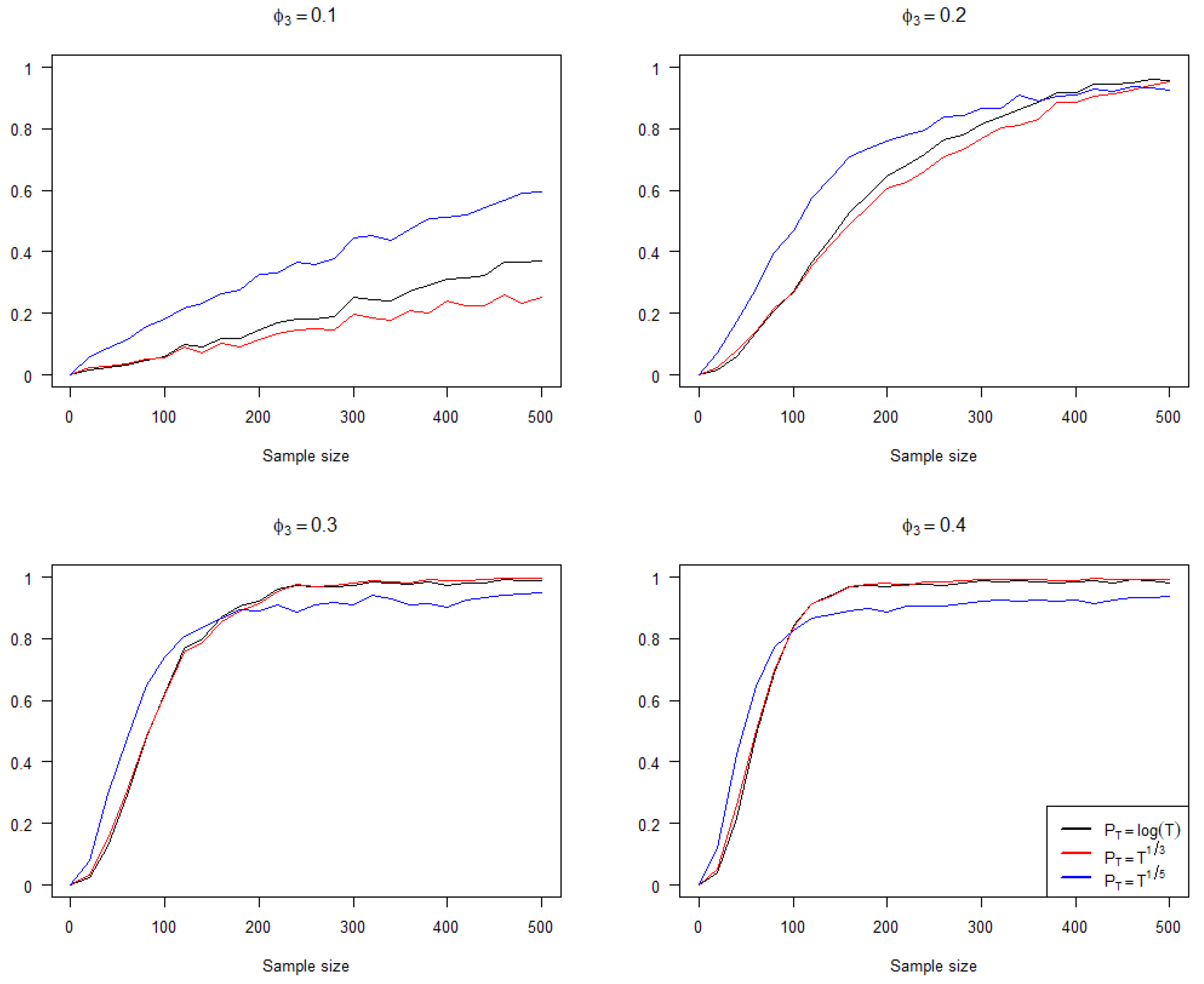
To investigate the performance of the three penalty terms under varying sample sizes and coefficient mean settings, we continue to consider model (7), where
follows a beta distribution with a mean of 0.4, and
follows a beta distribution with a mean of
. In
Figure 1, we report the impact of sample size on the accuracy of the penalized criteria using the three penalty terms under different
settings. In
Figure 1 and
Figure 2, the red line represents
, the black line represents
, and the blue line represents
, and the vertical axis of both figures represents the frequency of the penalized criteria (6) selecting the correct model. It can be observed that when
is small or the sample size is small, the performance of
is superior. However, as
gradually moves further from 0 and the sample size increases, the performance of
becomes slightly worse than
and
.
In
Figure 2, we report the frequency of selecting the model
using the penalized criteria (6) as
gradually varies from 0 to 0.4 under different sample size conditions. It should be noted that when
,
represents an incorrect model setting and the correct model setting, in this case, should be
. As shown in
Figure 2, when the sample size is small, particularly when the sample size is 100, the performance of
is notably improved compared to
and
. As the sample size increases, this advantage gradually diminishes, but the penalty term setting
still maintains an advantage when
is relatively close to 0.
Based on the numerical simulation results presented in this subsection, we can offer recommendations for applying the penalized criteria (6): when the sample size is small, or some coefficients in the true model are relatively close to 0, we can employ the penalty term setting
. In other cases, the performance of the penalty term settings
and
is comparable and slightly better than
. Furthermore, we also conducted a simulation study on lag variable selection for the data-generating process:
where the mean of
is 0.3. The results can be found in
Table A1 in
Appendix A.
3.2. Performance of Penalized Criteria in INARCH Models and AR Models
As stated in the Remark of
Section 2, we can apply the penalty criteria (6) to both INARCH and AR models. Because the likelihood functions for these two models can be easily established, we can compare the performance of the penalty criteria (6) with that of AIC and BIC for both these models.
3.2.1. INARCH Model
In this subsection, we consider the true data-generating process as follows:
where
,
, and
. Fokianos, Rahbek, and Tjøstheim [
26] proposed this model and derived the conditions for its stationarity and ergodicity. By applying the penalized criteria (6) alongside AIC and BIC, we attempt to select the true model from all INARCH models up to the third order. In
Table 2:
represents an i.i.d. Poisson random variable sequence,
represents the model ,
,
,
,
,
,
,
“Criterion” denotes the model selection criteria we use, and we use
to denote penalized criteria (6). Furthermore, we have bolded the true model
. We consider sample sizes
T = 100, 200, 300, 500, 1000, and for each sample size
T and parameter setting, we conduct 1000 independent repeated experiments.
From
Table 2, we can observe that, similar to the INAR case, the accuracy of
is slightly worse than
and
in larger sample sizes, but in smaller sample sizes, i.e.,
, the performance of
is superior. In addition, from
Table 2, we can observe that the accuracy of the penalized criteria proposed in this paper is roughly equivalent to BIC when
and
, while the accuracy is roughly equivalent to AIC in small samples when
, but
is far better than AIC when the sample size is large.
Table 2.
Frequency of model selection for INARCH model of order 2 by the penalized criterion (6).
Table 2.
Frequency of model selection for INARCH model of order 2 by the penalized criterion (6).
|
|---|
|
|---|
| Models to Be Selected |
|---|
| Criterion | | | | | | | | | |
|---|
| 100 | | | 0.059 | 0.576 | 0.001 | 0.019 | 0.021 | 0.309 | 0.001 | 0.014 |
| | | | 0.057 | 0.568 | 0.001 | 0.017 | 0.021 | 0.32 | 0.001 | 0.015 |
| | | | 0.012 | 0.337 | 0 | 0.007 | 0.054 | 0.509 | 0.003 | 0.078 |
| | | | 0.003 | 0.27 | 0 | 0.006 | 0.054 | 0.559 | 0.001 | 0.107 |
| | | | 0.032 | 0.551 | 0.002 | 0.021 | 0.022 | 0.361 | 0.001 | 0.01 |
| 200 | | | 0 | 0.406 | 0 | 0.002 | 0.013 | 0.574 | 0 | 0.005 |
| | | | 0 | 0.359 | 0 | 0.001 | 0.017 | 0.612 | 0 | 0.011 |
| | | | 0 | 0.138 | 0 | 0 | 0.028 | 0.756 | 0 | 0.078 |
| | | | 0 | 0.068 | 0 | 0 | 0.024 | 0.774 | 0 | 0.134 |
| | | | 0 | 0.296 | 0 | 0.001 | 0.019 | 0.673 | 0 | 0.011 |
| 300 | | | 0 | 0.22 | 0 | 0 | 0.07 | 0.767 | 0 | 0.006 |
| | | | 0 | 0.153 | 0 | 0 | 0.011 | 0.826 | 0 | 0.01 |
| | | | 0 | 0.041 | 0 | 0 | 0.01 | 0.874 | 0 | 0.075 |
| | | | 0 | 0.016 | 0 | 0 | 0.006 | 0.832 | 0 | 0.146 |
| | | | 0 | 0.127 | 0 | 0 | 0.008 | 0.855 | 0 | 0.01 |
| 500 | | | 0 | 0.035 | 0 | 0 | 0.03 | 0.958 | 0 | 0.004 |
| | | | 0 | 0.017 | 0 | 0 | 0.002 | 0.971 | 0 | 0.01 |
| | | | 0 | 0.001 | 0 | 0 | 0.002 | 0.934 | 0 | 0.063 |
| | | | 0 | 0 | 0 | 0 | 0.001 | 0.841 | 0 | 0.158 |
| | | | 0 | 0.012 | 0 | 0 | 0.004 | 0.976 | 0 | 0.008 |
| 1000 | | | 0 | 0 | 0 | 0 | 0 | 1 | 0 | 0 |
| | | | 0 | 0 | 0 | 0 | 0 | 0.991 | 0 | 0.009 |
| | | | 0 | 0 | 0 | 0 | 0 | 0.956 | 0 | 0.044 |
| | | | 0 | 0 | 0 | 0 | 0 | 0.848 | 0 | 0.152 |
| | | | 0 | 0 | 0 | 0 | 0 | 0.995 | 0 | 0.005 |
Additionally, we provide a simulation study on lag variable selection for the data-generating process:
The results can be found in
Table A2 in the
Appendix A.
3.2.2. AR Model
In this subsection, we consider the true data-generating process as follows:
where
,
,
, and
follows a normal distribution with a mean of 0 and a standard deviation of 2. By applying the penalized criteria (6) alongside AIC and BIC, we attempt to select the true model from all AR models up to the third order. In
Table 3:
represents an i.i.d. Normal random variable sequence,
represents the model ,
,
,
,
,
,
,
“Criterion” denotes the model selection criteria we use, and we use to denote penalized criteria (6). We use boldface to highlight the true model:
Table 3.
Frequency of model selection AR model of order 1 by the penalized criterion (6).
Table 3.
Frequency of model selection AR model of order 1 by the penalized criterion (6).
|
|---|
| Models to Be Selected |
|---|
| Criterion | | | | | | | | | |
|---|
| 100 | | | 0.048 | 0.577 | 0.002 | 0.02 | 0.018 | 0.324 | 0.001 | 0.01 |
| | | | 0.048 | 0.564 | 0.002 | 0.02 | 0.018 | 0.336 | 0.001 | 0.011 |
| | | | 0.009 | 0.34 | 0.002 | 0.012 | 0.044 | 0.524 | 0.001 | 0.068 |
| | | | 0.004 | 0.255 | 0.002 | 0.005 | 0.059 | 0.578 | 0.002 | 0.095 |
| | | | 0.032 | 0.564 | 0.001 | 0.016 | 0.018 | 0.352 | 0.001 | 0.016 |
| 200 | | | 0.001 | 0.323 | 0 | 0.001 | 0.011 | 0.654 | 0 | 0.01 |
| | | | 0.001 | 0.279 | 0 | 0 | 0.014 | 0.693 | 0 | 0.013 |
| | | | 0 | 0.11 | 0 | 0 | 0.025 | 0.79 | 0 | 0.075 |
| | | | 0 | 0.062 | 0 | 0 | 0.021 | 0.771 | 0 | 0.146 |
| | | | 0.001 | 0.261 | 0 | 0 | 0.013 | 0.713 | 0 | 0.012 |
| 300 | | | 0 | 0.167 | 0 | 0 | 0.004 | 0.825 | 0 | 0.004 |
| | | | 0 | 0.116 | 0 | 0 | 0.004 | 0.874 | 0 | 0.006 |
| | | | 0 | 0.042 | 0 | 0 | 0.007 | 0.893 | 0 | 0.058 |
| | | | 0 | 0.017 | 0 | 0 | 0.007 | 0.824 | 0 | 0.152 |
| | | | 0 | 0.107 | 0 | 0 | 0.005 | 0.88 | 0 | 0.008 |
| 500 | | | 0 | 0.034 | 0 | 0 | 0.003 | 0.959 | 0 | 0.004 |
| | | | 0 | 0.013 | 0 | 0 | 0.004 | 0.975 | 0 | 0.008 |
| | | | 0 | 0.002 | 0 | 0 | 0.001 | 0.937 | 0 | 0.06 |
| | | | 0 | 0 | 0 | 0 | 0 | 0.837 | 0 | 0.163 |
| | | | 0 | 0.011 | 0 | 0 | 0.003 | 0.977 | 0 | 0.009 |
| 1000 | | | 0 | 0 | 0 | 0 | 0 | 0.996 | 0 | 0.004 |
| | | | 0 | 0 | 0 | 0 | 0 | 0.989 | 0 | 0.011 |
| | | | 0 | 0 | 0 | 0 | 0 | 0.951 | 0 | 0.046 |
| | | | 0 | 0 | 0 | 0 | 0 | 0.846 | 0 | 0.154 |
| | | | 0 | 0 | 0 | 0 | 0 | 0.988 | 0 | 0.012 |
From
Table 3, we can observe that, similar to the INAR case, the accuracy of
is slightly worse than
and
in larger sample sizes, but in smaller sample sizes, i.e.,
, the performance of
is superior. The comparison of the penalized criteria proposed in this paper with AIC and BIC in the AR model is analogous to that in the INARCH model; thus further elaboration is not required.
3.3. Robustness of Variable Selection Procedure
In this section, we investigate the robustness of the penalized criteria (6) for different distributions of the innovation term
in model (7). Specifically, we consider
to follow a Poisson distribution, a geometric distribution with a mean of 2, and a uniform distribution over
. In
Table 4, “
” denotes the random distribution of the innovation term, whereas “geom” denotes the geometric distribution.
Through
Table 4, we observe that the penalized criteria (6) remain robust for various distributions of the innovation term
. This finding suggests that the criteria proposed in this paper can effectively select the correct lag order even when the innovation term adheres to different distributions. We use boldface to highlight the true model:
Table 4.
Frequency of model selection of INAR model by the penalized criterion (6) with misspecification.
Table 4.
Frequency of model selection of INAR model by the penalized criterion (6) with misspecification.
|
|---|
| Models to Be Selected |
|---|
| | | | | | | | | | |
|---|
| 100 | Poisson | | 0.045 | 0.587 | 0.003 | 0.018 | 0.018 | 0.319 | 0 | 0.01 |
| | | | 0.043 | 0.584 | 0.003 | 0.019 | 0.018 | 0.323 | 0 | 0.01 |
| | | | 0.005 | 0.349 | 0.002 | 0.008 | 0.053 | 0.514 | 0.003 | 0.066 |
| | Uniform | | 0.048 | 0.564 | 0.001 | 0.02 | 0.018 | 0.336 | 0.001 | 0.048 |
| | | | 0.043 | 0.559 | 0 | 0.019 | 0.02 | 0.345 | 0.001 | 0.043 |
| | | | 0.014 | 0.332 | 0 | 0.004 | 0.047 | 0.519 | 0 | 0.014 |
| | Geom | | 0.07 | 0.575 | 0.004 | 0.032 | 0.023 | 0.285 | 0.001 | 0.02 |
| | | | 0.067 | 0.57 | 0.004 | 0.032 | 0.024 | 0.292 | 0.001 | 0.02 |
| | | | 0.009 | 0.327 | 0.002 | 0.011 | 0.052 | 0.511 | 0.002 | 0.086 |
| 200 | Poisson | | 0 | 0.37 | 0 | 0.001 | 0.008 | 0.612 | 0 | 0.008 |
| | | | 0 | 0.319 | 0 | 0.002 | 0.012 | 0.655 | 0 | 0.012 |
| | | | 0 | 0.109 | 0 | 0.001 | 0.02 | 0.795 | 0 | 0.075 |
| | Uniform | | 0 | 0.343 | 0 | 0 | 0.012 | 0.636 | 0 | 0.009 |
| | | | 0 | 0.29 | 0 | 0 | 0.016 | 0.681 | 0 | 0.013 |
| | | | 0 | 0.13 | 0 | 0 | 0.026 | 0.776 | 0 | 0.068 |
| | Geom | | 0.005 | 0.358 | 0 | 0 | 0.018 | 0.603 | 0 | 0.016 |
| | | | 0.004 | 0.312 | 0 | 0 | 0.02 | 0.643 | 0 | 0.021 |
| | | | 0 | 0.108 | 0 | 0 | 0.034 | 0.752 | 0 | 0.106 |
| 300 | Poisson | | 0 | 0.193 | 0 | 0 | 0.003 | 0.801 | 0 | 0.003 |
| | | | 0 | 0.138 | 0 | 0 | 0.004 | 0.852 | 0 | 0.006 |
| | | | 0 | 0.044 | 0 | 0 | 0.005 | 0.878 | 0 | 0.073 |
| | Uniform | | 0 | 0.184 | 0 | 0 | 0.01 | 0.802 | 0 | 0.004 |
| | | | 0 | 0.122 | 0 | 0 | 0.012 | 0.851 | 0 | 0.015 |
| | | | 0 | 0.03 | 0 | 0 | 0.011 | 0.885 | 0 | 0.074 |
| | Geom | | 0 | 0.188 | 0 | 0 | 0.012 | 0.796 | 0 | 0.004 |
| | | | 0 | 0.133 | 0 | 0 | 0.015 | 0.834 | 0 | 0.018 |
| | | | 0 | 0.027 | 0 | 0 | 0.013 | 0.88 | 0 | 0.08 |
| 500 | Poisson | | 0 | 0.027 | 0 | 0 | 0.005 | 0.962 | 0 | 0.006 |
| | | | 0 | 0.008 | 0 | 0 | 0.005 | 0.975 | 0 | 0.012 |
| | | | 0 | 0.002 | 0 | 0 | 0.003 | 0.923 | 0 | 0.072 |
| | Uniform | | 0 | 0.04 | 0 | 0 | 0.004 | 0.95 | 0 | 0.006 |
| | | | 0 | 0.02 | 0 | 0 | 0.002 | 0.964 | 0 | 0.014 |
| | | | 0 | 0.003 | 0 | 0 | 0 | 0.926 | 0 | 0.071 |
| | Geom | | 0 | 0.035 | 0 | 0 | 0.008 | 0.954 | 0 | 0.003 |
| | | | 0 | 0.018 | 0 | 0 | 0.007 | 0.964 | 0 | 0.011 |
| | | | 0 | 0.002 | 0 | 0 | 0.003 | 0.928 | 0 | 0.067 |
| 1000 | Poisson | | 0 | 0 | 0 | 0 | 0 | 0.998 | 0 | 0.002 |
| | | | 0 | 0 | 0 | 0 | 0 | 0.989 | 0 | 0.011 |
| | | | 0 | 0 | 0 | 0 | 0 | 0.952 | 0 | 0.048 |
| | Uniform | | 0 | 0 | 0 | 0 | 0 | 1 | 0 | 0 |
| | | | 0 | 0 | 0 | 0 | 0 | 0.995 | 0 | 0.05 |
| | | | 0 | 0 | 0 | 0 | 0 | 0.944 | 0 | 0.056 |
| | Geom | | 0 | 0 | 0 | 0 | 0 | 0.994 | 0 | 0.006 |
| | | | 0 | 0 | 0 | 0 | 0 | 0.982 | 0 | 0.018 |
| | | | 0 | 0 | 0 | 0 | 0 | 0.947 | 0 | 0.053 |
Furthermore, we compare the performance of the penalized criteria proposed in this paper, AIC, and BIC when the innovation term
in AR model (8) follows a uniform distribution over [−2, 2] while the assumption of
is a normal distribution with mean 0 and unknown variance
. In
Appendix A,
Table A3 shows that regardless of the distribution of the innovation term, when the conditional mean is set correctly, the performance and robustness of the penalized criteria proposed in this paper are generally equivalent to those of AIC and BIC.
5. Discussion and Conclusions
In this paper, we propose a model selection criterion based on an estimation equation established in Conditional Least Squares estimation. This penalized method does not rely on detailed distributional assumptions for the data-generating process. It circumvents the complex likelihood function construction in Random Coefficient Integer-Valued Autoregressive models and can consistently select the correct variables under relatively mild assumptions.
In our numerical simulations, we compared the impact of three penalty term settings on the performance of the penalty criteria. We found that the impact of these penalty terms on the performance of the information criteria varies as partial coefficients in the RCINAR model move farther away from 0 or as the sample size increases. Moreover, we applied the model selection method proposed in this paper to both the INARCH and traditional continuous-valued AR models. We discovered that in both scenarios where likelihood functions can be easily constructed, the proposed model selection criteria and the traditional likelihood-based information criteria, AIC and BIC, exhibit similar model selection efficiency. Specifically, under the settings of and , the accuracy of the proposed model selection method is similar to that of BIC. However, in cases with smaller sample sizes, the proposed model selection method with performs similarly to AIC while outperforming AIC with larger sample sizes.
In the future, model selection methods based on estimation equations have considerable potential for development. In this discussion section, we briefly introduce three aspects:
- (1)
Distinguishing between different thinning operators or innovation terms with varying distributions: The criterion (6) provided in this paper is primarily used for lag variable selection but lacks the ability to differentiate between various thinning operators and distinct distributions of innovation terms. It is well known that INAR models can describe scenarios such as zero inflation, variance inflation, and extreme values by flexibly selecting thinning operators and innovation terms. Therefore, if a model selection criterion can distinguish between different thinning operators and varying distributions of innovation terms, it will have a more extensive application scope.
- (2)
Incorporating higher-order conditional moments from the data-generating process into the information criterion. Through the form of the
function:
It is evident that criterion (6) only contains the mean structure information of the model and lacks the ability to describe higher-order moment information. Since many variants of the INAR model exhibit differences in higher-order moments, incorporating higher-order moment information into the model selection criterion would enable criterion (6) to perform model selection within a broader context.
- (3)
Detecting change points. In the field of time series data research, the change point detection problem has a long history. Specifically, within the integer-valued time series domain, the change point problem refers to the existence of positive integers
, such that:
For continuous-valued time series models, Chen and Gupta [
28] introduced a method for change point detection using AIC and BIC. Since parameter changes are prominently reflected in the mean structure of INAR models, it is likely feasible to perform change point detection using the criterion (6) based on the estimation equations.


