
Far from Asymptopia: Unbiased High-Dimensional Inference Cannot Assume Unlimited Data


Abstract
1. Introduction
2. Results
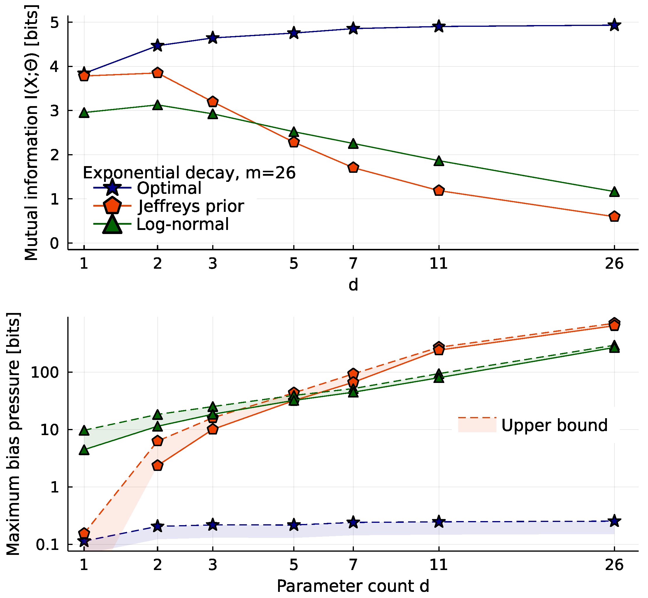
2.1. Exponential Decay Models
2.2. The Costs of High Dimensionality
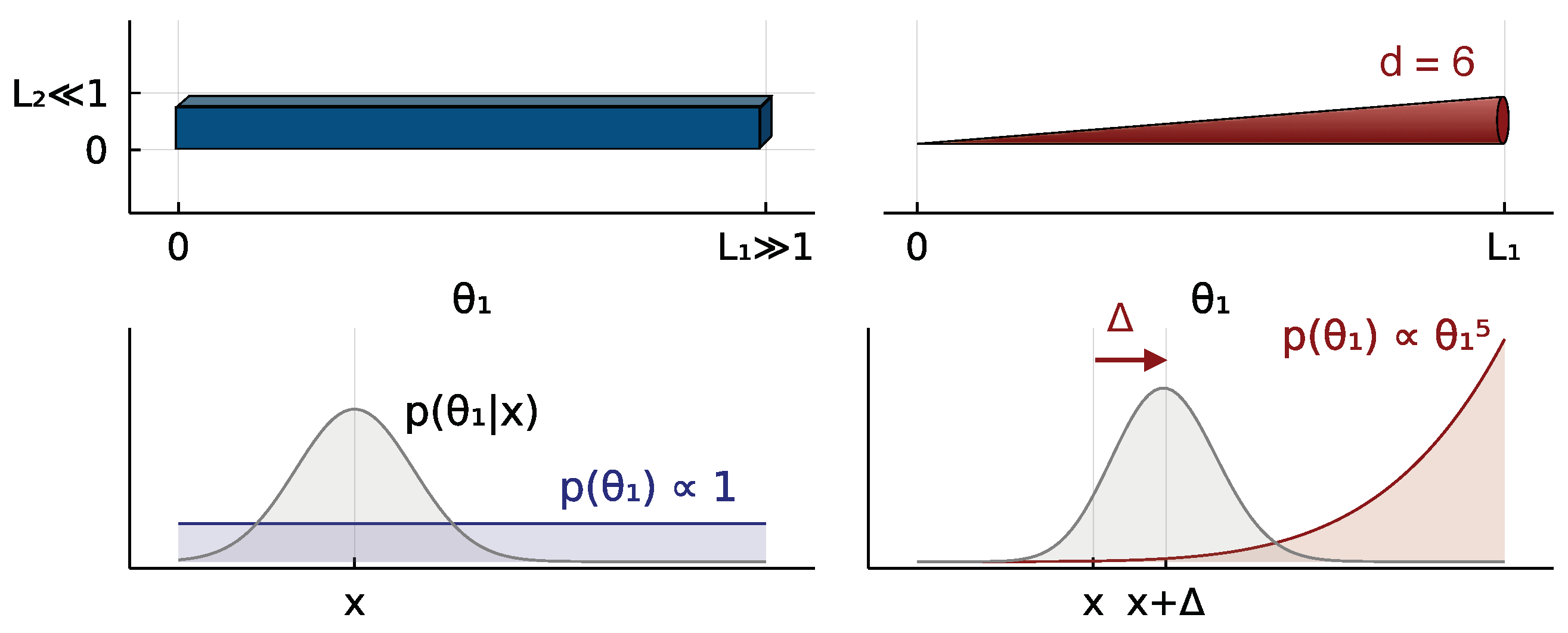
2.3. Inequivalent Parameters
3. Discussion
Author Contributions
Funding
Institutional Review Board Statement
Informed Consent Statement
Data Availability Statement
Acknowledgments
Conflicts of Interest
Appendix A
Appendix A.1. Square Hypercone

Appendix A.2. Estimating I(X;Θ) and Its Gradient
Appendix A.3. Other Methods
- More recently, the following lower bound for was used by [41] to find approximations to :This bound is too crude to see the features of interest here: For all models in this paper, it favors a prior with just two delta functions, for any noise level .
- We mentioned above that adjusting some “meta-parameters” of some distribution would be one way to handle near-optimal priors. This is the approach of [41], and of many papers maximizing other scores, often described as “variational”.
- Another prior that typically has large was introduced in [6] under the name “adaptive slab-and-spike prior”. It pulls every point x in a distributionback to its maximum likelihood point :The result has weight everywhere in the model manifold, but has extra weight on the edges. Because the amount of weight on edges is controlled by , it adopts an appropriate effective dimensionality (8), and has a low bias (5).
Appendix A.4. Bias Alla Bennett
Appendix A.5. Jeffreys and Vandermonde
Appendix A.6. Michaelis–Menten et al.
Appendix A.7. Ever since the Big Bang
Appendix A.8. Terminology
References
- Rao, C.R. Information and accuracy attainable in the estimation of statistical parameters. Bull. Calcutta Math. Soc. 1945, 37, 81–91. [Google Scholar]
- Amari, S.I. A foundation of information geometry. Electron. Commun. Jpn. 1983, 66, 1–10. [Google Scholar] [CrossRef]
- Brown, K.S.; Sethna, J.P. Statistical mechanical approaches to models with many poorly known parameters. Phys. Rev. E 2003, 68, 021904. [Google Scholar] [CrossRef]
- Daniels, B.C.; Chen, Y.J.; Sethna, J.P.; Gutenkunst, R.N.; Myers, C.R. Sloppiness, robustness, and evolvability in systems biology. Curr. Opin. Biotechnol. 2008, 19, 389–395. [Google Scholar] [CrossRef]
- Machta, B.B.; Chachra, R.; Transtrum, M.K.; Sethna, J.P. Parameter space compression underlies emergent theories and predictive models. Science 2013, 342, 604–607. [Google Scholar] [CrossRef]
- Quinn, K.N.; Abbott, M.C.; Transtrum, M.K.; Machta, B.B.; Sethna, J.P. Information geometry for multiparameter models: New perspectives on the origin of simplicity. Rep. Prog. Phys. 2023, 86, 035901. [Google Scholar] [CrossRef]
- Lindley, D.V. The use of prior probability distributions in statistical inference and decisions. In Proceedings of the Fourth Berkeley Symposium on Mathematical Statistics and Probability, Berkeley, CA, USA, 30 June–30 July 1961. [Google Scholar]
- Bernardo, J.M. Reference posterior distributions for Bayesian inference. J. Roy. Stat. Soc. B 1979, 41, 113–128. [Google Scholar] [CrossRef]
- Mattingly, H.H.; Transtrum, M.K.; Abbott, M.C.; Machta, B.B. Maximizing the information learned from finite data selects a simple model. Proc. Natl. Acad. Sci. USA 2018, 115, 1760–1765. [Google Scholar] [CrossRef]
- Kashyap, R. Prior probability and uncertainty. IEEE Trans. Inform. Theory 1971, 17, 641–650. [Google Scholar] [CrossRef]
- Haussler, D. A general minimax result for relative entropy. IEEE Trans. Inform. Theory 1997, 43, 1276–1280. [Google Scholar] [CrossRef]
- Krob, J.; Scholl, H.R. A minimax result for the Kullback Leibler Bayes risk. Econ. Qual. Control 1997, 12, 147–157. [Google Scholar]
- Färber, G. Die Kanalkapazität allgemeiner Übertragunskanäle bei begrenztem Signalwertbereich beliebigen Signalübertragungszeiten sowie beliebiger Störung. Arch. Elektr. Übertr. 1967, 21, 565–574. [Google Scholar]
- Smith, J.G. The information capacity of amplitude-and variance-constrained scalar gaussian channels. Inf. Control. 1971, 18, 203–219. [Google Scholar] [CrossRef]
- Berger, J.O.; Bernardo, J.M.; Mendoza, M. On priors that maximize expected information. In Recent Developments in Statistics and Their Applications; Seoul Freedom Academy Publishing: Seoul, Republic of Korea, 1989. [Google Scholar]
- Zhang, Z. Discrete Noninformative Priors. Ph.D. Thesis, Yale University, New Haven, CT, USA, 1994. [Google Scholar]
- Scholl, H.R. Shannon optimal priors on independent identically distributed statistical experiments converge weakly to Jeffreys’ prior. Test 1998, 7, 75–94. [Google Scholar] [CrossRef]
- Sims, C.A. Rational inattention: Beyond the linear-quadratic case. Am. Econ. Rev. 2006, 96, 158–163. [Google Scholar] [CrossRef]
- Connes, A. Noncommutative Geometry; Academic Press: San Diego, CA, USA, 1994. [Google Scholar]
- Jeffreys, H. An invariant form for the prior probability in estimation problems. Proc. R. Soc. Lond. A 1946, 186, 453–461. [Google Scholar] [CrossRef]
- Clarke, B.S.; Barron, A.R. Jeffreys’ prior is asymptotically least favorable under entropy risk. J. Stat. Plan. Inference 1994, 41, 37–60. [Google Scholar] [CrossRef]
- Balasubramanian, V. Statistical inference, Occam’s razor, and statistical mechanics on the space of probability distributions. Neural Comput. 1997, 9, 349–368. [Google Scholar] [CrossRef]
- Transtrum, M.K.; Machta, B.B.; Sethna, J.P. Why are nonlinear fits to data so challenging? Phys. Rev. Lett. 2010, 104, 060201. [Google Scholar] [CrossRef]
- Clarke, B.; Barron, A. Information-theoretic asymptotics of Bayes methods. IEEE Trans. Inform. Theory 1990, 36, 453–471. [Google Scholar] [CrossRef]
- Abbott, M.C.; Machta, B.B. A scaling law from discrete to continuous solutions of channel capacity problems in the low-noise limit. J. Stat. Phys. 2019, 176, 214–227. [Google Scholar] [CrossRef]
- Bennett, C.H. Efficient estimation of free energy differences from Monte Carlo data. J. Comput. Phys 1976, 22, 245–268. [Google Scholar] [CrossRef]
- Hines, K.E.; Middendorf, T.R.; Aldrich, R.W. Determination of parameter identifiability in nonlinear biophysical models: A Bayesian approach. J. Gen. Physiol. 2014, 143, 401–416. [Google Scholar] [CrossRef] [PubMed]
- Transtrum, M.K.; Qiu, P. Bridging mechanistic and phenomenological models of complex biological systems. PLoS Comput. Biol. 2016, 12, e1004915. [Google Scholar] [CrossRef]
- Akaike, H. A new look at the statistical model identification. IEEE Trans. Automat. Contr. 1974, 19, 716–723. [Google Scholar] [CrossRef]
- Rissanen, J. Modeling by shortest data description. Automatica 1978, 14, 465–471. [Google Scholar] [CrossRef]
- Grünwald, P.; Roos, T. Minimum description length revisited. Int. J. Math. Ind. 2019, 11, 1930001. [Google Scholar] [CrossRef]
- Schwarz, G. Estimating the dimension of a model. Ann. Statist. 1978, 6, 461–464. [Google Scholar] [CrossRef]
- Myung, I.J.; Balasubramanian, V.; Pitt, M.A. Counting probability distributions: Differential geometry and model selection. Proc. Natl. Acad. Sci. USA 2000, 97, 11170–11175. [Google Scholar] [CrossRef]
- Piasini, E.; Balasubramanian, V.; Gold, J.I. Effect of geometric complexity on intuitive model selection. In Machine Learning, Optimization, and Data Science; Springer: Berlin/Heidelberg, Germany, 2022; pp. 1–24. [Google Scholar] [CrossRef]
- O’Leary, T.; Williams, A.H.; Caplan, J.S.; Marder, E. Correlations in ion channel expression emerge from homeostatic tuning rules. Proc. Natl. Acad. Sci. USA 2013, 110, E2645–E2654. [Google Scholar] [CrossRef]
- Wen, M.; Shirodkar, S.N.; Plecháč, P.; Kaxiras, E.; Elliott, R.S.; Tadmor, E.B. A force-matching Stillinger-Weber potential for MoS2: Parameterization and Fisher information theory based sensitivity analysis. J. Appl. Phys. 2017, 122, 244301. [Google Scholar] [CrossRef]
- Marschmann, G.L.; Pagel, H.; Kügler, P.; Streck, T. Equifinality, sloppiness, and emergent structures of mechanistic soil biogeochemical models. Environ. Model. Softw. 2019, 122, 104518. [Google Scholar] [CrossRef]
- Karakida, R.; Akaho, S.; Amari, S.i. Pathological spectra of the Fisher information metric and its variants in deep neural networks. Neural Comput. 2021, 33, 2274–2307. [Google Scholar] [CrossRef] [PubMed]
- Kadanoff, L.P. Scaling laws for Ising models near Tc. Physics 1966, 2, 263–272. [Google Scholar] [CrossRef]
- Wilson, K.G. Renormalization group and critical phenomena. 1. Renormalization group and the Kadanoff scaling picture. Phys. Rev. 1971, B4, 3174–3183. [Google Scholar] [CrossRef]
- Nalisnick, E.; Smyth, P. Learning approximately objective priors. arXiv 2017, arXiv:1704.01168. [Google Scholar]
- Bezanson, J.; Karpinski, S.; Shah, V.B.; Edelman, A. Julia: A fast dynamic language for technical computing. arXiv 2012, arXiv:1209.5145. [Google Scholar]
- Huber, M.F.; Bailey, T.; Durrant-Whyte, H.; Hanebeck, U.D. On entropy approximation for Gaussian mixture random vectors. In Proceedings of the 2008 IEEE International Conference on Multisensor Fusion and Integration for Intelligent Systems, Seoul, Republic of Korea, 20–22 August 2008; pp. 181–188. [Google Scholar] [CrossRef]
- Nocedal, J. Updating quasi-Newton matrices with limited storage. Math. Comp. 1980, 35, 773–782. [Google Scholar] [CrossRef]
- Johnson, S.G. The NLopt Nonlinear-Optimization Package. Available online: http://github.com/stevengj/nlopt (accessed on 6 May 2022).
- Mitchell, D.P. Spectrally optimal sampling for distribution ray tracing. SIGGRAPH Comput. Graph. 1991, 25, 157–164. [Google Scholar] [CrossRef]
- Blahut, R. Computation of channel capacity and rate-distortion functions. IEEE Trans. Inform. Theory 1972, 18, 460–473. [Google Scholar] [CrossRef]
- Arimoto, S. An algorithm for computing the capacity of arbitrary discrete memoryless channels. IEEE Trans. Inform. Theory 1972, 18, 14–20. [Google Scholar] [CrossRef]
- Lafferty, J.; Wasserman, L.A. Iterative Markov chain Monte Carlo computation of reference priors and minimax risk. Uncertain. AI 2001, 17, 293–300. [Google Scholar]
- Goodman, J.; Weare, J. Ensemble samplers with affine invariance. CAMCoS 2010, 5, 65–80. [Google Scholar] [CrossRef]
- Ma, Y.; Dixit, V.; Innes, M.; Guo, X.; Rackauckas, C. A comparison of automatic differentiation and continuous sensitivity analysis for derivatives of differential equation solutions. arXiv 2021, arXiv:1812.01892. [Google Scholar]
- Michaelis, L.; Menten, M.L. Die Kinetik der Invertinwirkung. Biochem. Z 1913, 49, 333–369. [Google Scholar]
- Briggs, G.E.; Haldane, J.B.S. A note on the kinetics of enzyme action. Biochem. J. 1925, 19, 338–339. [Google Scholar] [CrossRef]
- Schnell, S.; Mendoza, C. Closed Form Solution for Time-dependent Enzyme Kinetics. J. Theor. Biol. 1997, 187, 207–212. [Google Scholar] [CrossRef]
- Planck Collaboration. Planck 2018 results. VI. Cosmological parameters. Astron. Astrophys. 2021, 641, A6. [Google Scholar] [CrossRef]
- Kass, R.E.; Wasserman, L. The selection of prior distributions by formal rules. J. Am. Stat. Assoc. 1996, 91, 1343–1370. [Google Scholar] [CrossRef]


Disclaimer/Publisher’s Note: The statements, opinions and data contained in all publications are solely those of the individual author(s) and contributor(s) and not of MDPI and/or the editor(s). MDPI and/or the editor(s) disclaim responsibility for any injury to people or property resulting from any ideas, methods, instructions or products referred to in the content. |
© 2023 by the authors. Licensee MDPI, Basel, Switzerland. This article is an open access article distributed under the terms and conditions of the Creative Commons Attribution (CC BY) license (https://creativecommons.org/licenses/by/4.0/).
Share and Cite
Abbott, M.C.; Machta, B.B. Far from Asymptopia: Unbiased High-Dimensional Inference Cannot Assume Unlimited Data. Entropy 2023, 25, 434. https://doi.org/10.3390/e25030434
Abbott MC, Machta BB. Far from Asymptopia: Unbiased High-Dimensional Inference Cannot Assume Unlimited Data. Entropy. 2023; 25(3):434. https://doi.org/10.3390/e25030434
Chicago/Turabian StyleAbbott, Michael C., and Benjamin B. Machta. 2023. "Far from Asymptopia: Unbiased High-Dimensional Inference Cannot Assume Unlimited Data" Entropy 25, no. 3: 434. https://doi.org/10.3390/e25030434
APA StyleAbbott, M. C., & Machta, B. B. (2023). Far from Asymptopia: Unbiased High-Dimensional Inference Cannot Assume Unlimited Data. Entropy, 25(3), 434. https://doi.org/10.3390/e25030434