
Expecting the Unexpected: Entropy and Multifractal Systems in Finance


Abstract
1. Introduction
2. Materials and Methods
2.1. Data
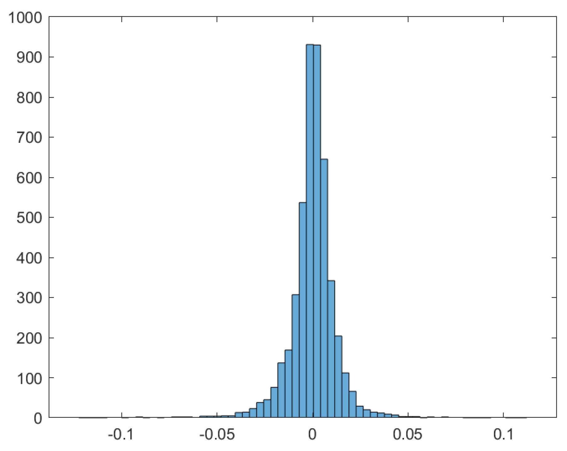
2.1.1. Real Data
2.1.2. Simulated Data
2.2. Sample Entropy
- Parameters
2.3. Spectral Analysis
2.4. Multifractality and Determinism
2.5. Segmentation and Correlation
3. Results and Analysis
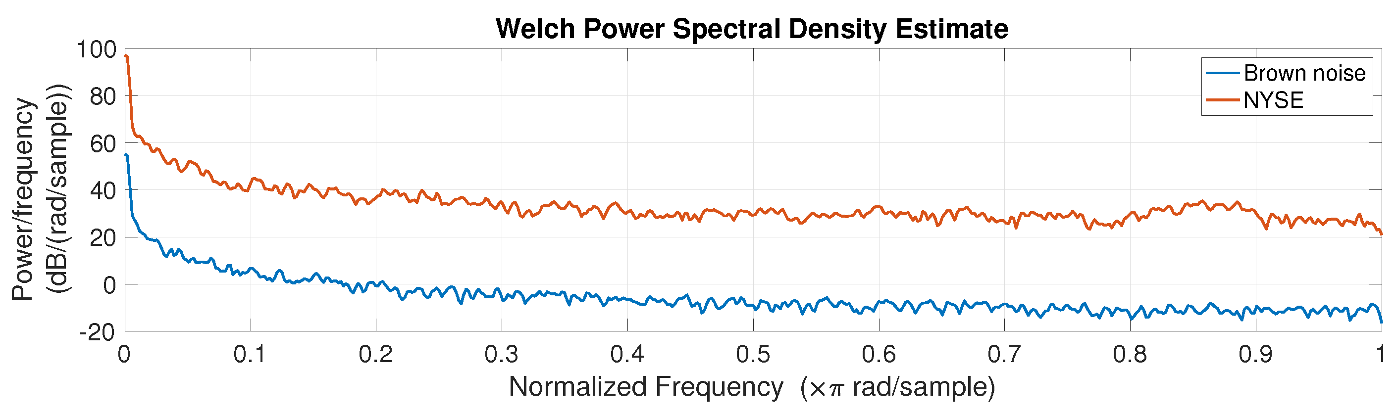
3.1. Power Spectral Density
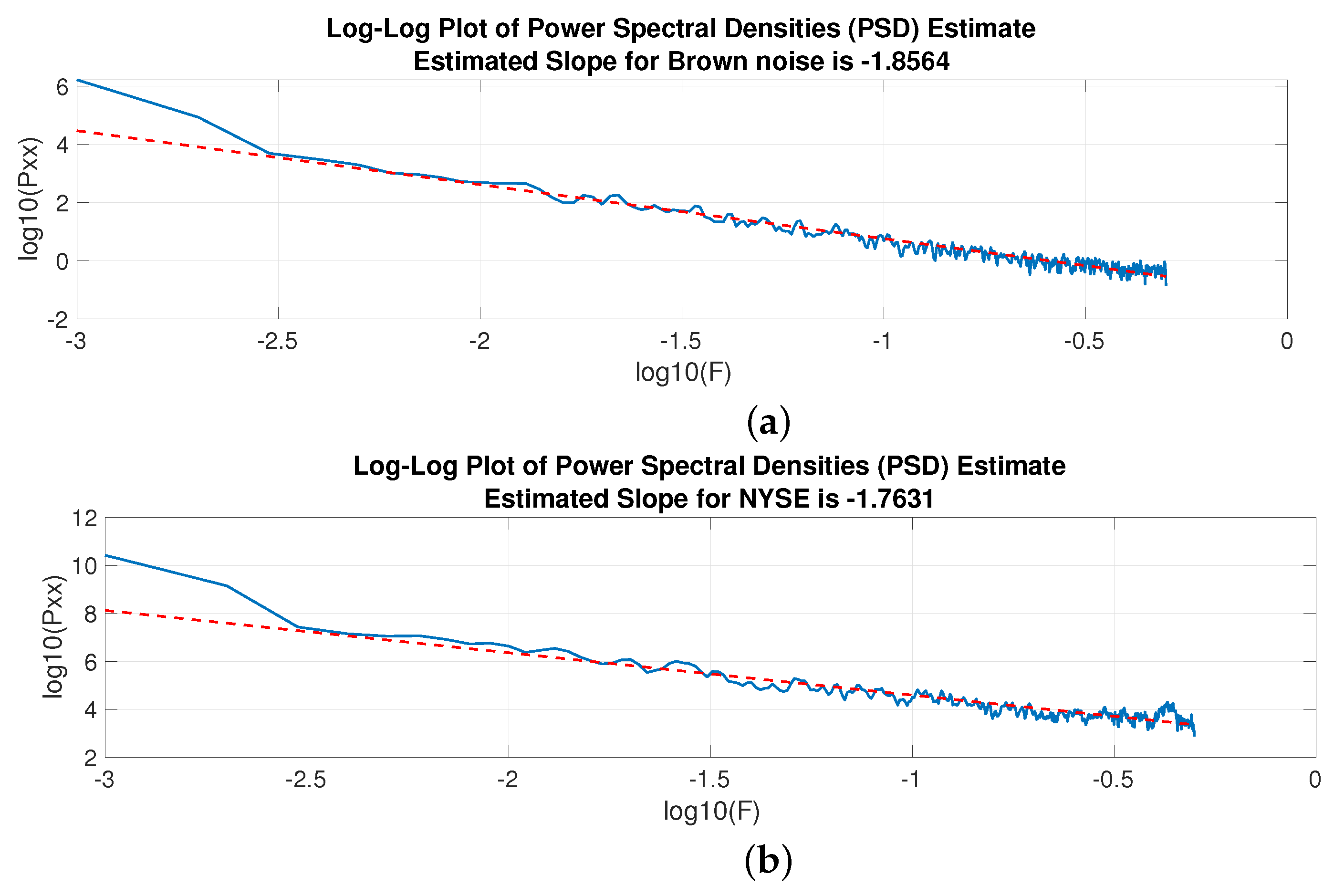
3.2. Power Law Process Estimation
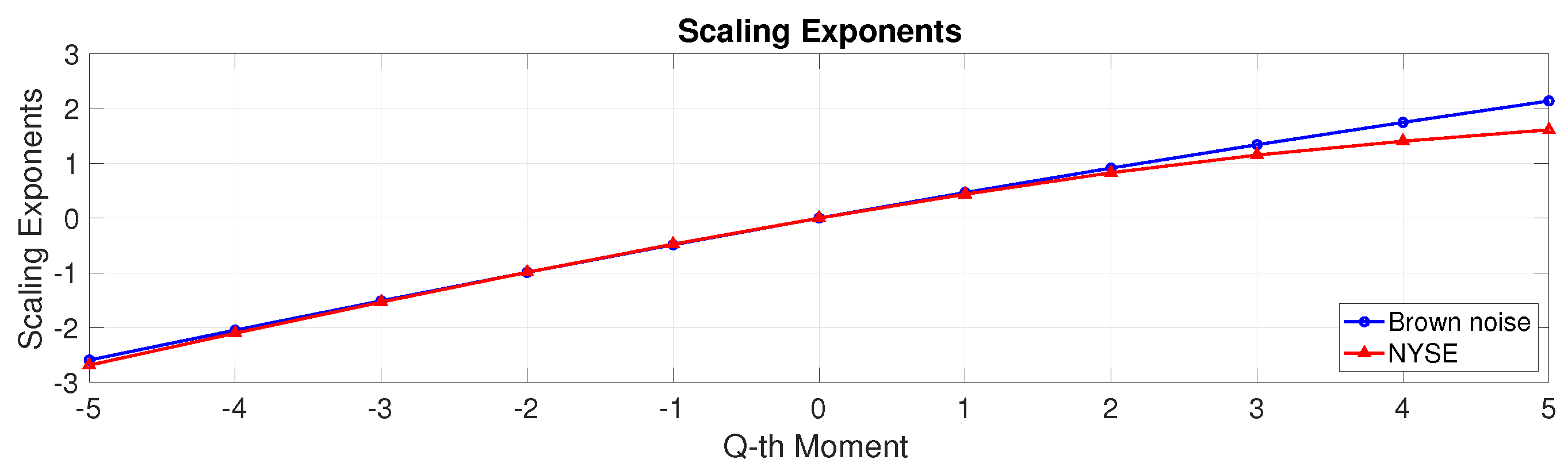
3.3. Multifractal Analysis
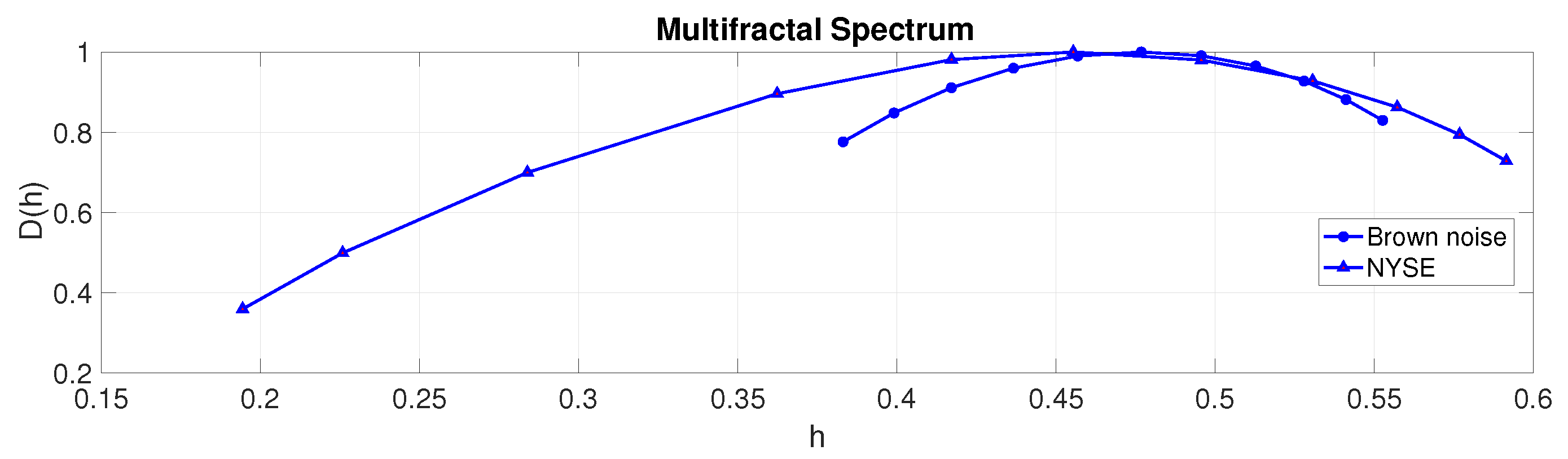
3.4. Multifractal Spectrum
3.5. Entropy
4. Conclusions
Author Contributions
Funding
Data Availability Statement
Acknowledgments
Conflicts of Interest
Appendix A. RR Interval and QRS Complex
Appendix B. Entropy Sensitivity Analysis

| Embedded Dimension | Tolerance | ||
|---|---|---|---|
| 1 | 0.4 std(dtrd(NYSE)) | 1.3739 | 5.4112 |
| 2 | 0.4 std(dtrd(NYSE)) | 1.2504 | 5.4112 |
| 3 | 0.4 std(dtrd(NYSE)) | 1.0909 | 16.323 |
| 1 | 0.3 std(dtrd(NYSE)) | 1.6410 | 5.6300 |
| 2 | 0.3 std(dtrd(NYSE)) | 1.4751 | 16.324 |
| 3 | 0.3 std(dtrd(NYSE)) | 1.2171 | NaN |
| 1 | 0.2 std(dtrd(NYSE)) | 2.0146 | 5.9674 |
| 2 | 0.2 std(dtrd(NYSE)) | 1.7407 | 16.324 |
| 3 | 0.2 std(dtrd(NYSE)) | 1.2514 | NaN |
| 1 | 0.02 std(dtrd(NYSE)) | 3.3943 | 16.324 |
| 2 | 0.02 std(dtrd(NYSE)) | 0.7004 | NaN |
| 3 | 0.02 std(dtrd(NYSE)) | 0.0208 | NaN |
| 1 | 0.002 std(dtrd(NYSE)) | 1.9683 | 16.324 |
| 2 | 0.002 std(dtrd(NYSE)) | 0.0108 | NaN |
| 3 | 0.002 std(dtrd(NYSE)) | −0.0002 | NaN |
| Embedded Dimension | Tolerance | ||
|---|---|---|---|
| 1 | 0.4 std(dtrd(BN)) | 1.6412 | 8.8103 |
| 2 | 0.4 std(dtrd(BN)) | 1.6345 | 20.101 |
| 3 | 0.4 std(dtrd(BN)) | 1.6013 | NaN |
| 1 | 0.3 std(dtrd(BN)) | 1.9272 | 8.9028 |
| 2 | 0.3 std(dtrd(BN)) | 1.9115 | 20.101 |
| 3 | 0.3 std(dtrd(BN)) | 1.8220 | NaN |
| 1 | 0.2 std(dtrd(BN)) | 2.3290 | 9.6780 |
| 2 | 0.2 std(dtrd(BN)) | 2.2828 | 20.101 |
| 3 | 0.2 std(dtrd(BN)) | 1.9870 | NaN |
| 1 | 0.02 std(dtrd(BN)) | 4.3411 | 20.101 |
| 2 | 0.02 std(dtrd(BN)) | 1.3888 | NaN |
| 3 | 0.02 std(dtrd(BN)) | 0.0321 | NaN |
| 1 | 0.002 std(dtrd(BN)) | 3.4545 | 20.101 |
| 2 | 0.002 std(dtrd(BN)) | 0.0292 | NaN |
| 3 | 0.002 std(dtrd(BN)) | 0.00001 | NaN |
References
- Zhou, R.; Cai, R.; Tong, G. Applications of Entropy in Finance: A Review. Entropy 2013, 15, 4909–4931. [Google Scholar] [CrossRef]
- Jorion, P. Risk Management Lessons from the Credit Crisis. Eur. Financ. Manag. 2009, 15, 923–933. [Google Scholar] [CrossRef]
- NASA-Space and Technology-Subcommittee on Space. NASA Program Management and Procurement Procedures and Practices: Hearings Before the Subcommittee on Space Science and Applications of the Committee on Science and Technology, U.S. House of Representatives, Ninety-seventh Congress, First Session, June 24, 25, 1981; US Government Printing Office: Washington, DC, USA, 1981; Number 16.
- Orlando, G. Coping with Risk and Uncertainty in Contemporary Economic Thought. 2022. Available online: https://papers.ssrn.com/sol3/papers.cfm?abstract_id=4209287 (accessed on 1 October 2023).
- Frittelli, M. The Minimal Entropy Martingale Measure and the Valuation Problem in Incomplete Markets. Math. Financ. 2000, 10, 39–52. [Google Scholar] [CrossRef]
- Geman, D.; Geman, H.; Taleb, N.N. Tail Risk Constraints and Maximum Entropy. Entropy 2015, 17, 3724–3737. [Google Scholar] [CrossRef]
- Kelbert, M.; Stuhl, I.; Suhov, Y. Weighted entropy and optimal portfolios for risk-averse Kelly investments. Aequationes Math. 2018, 92, 165–200. [Google Scholar] [CrossRef]
- Patel, P.; Raghunandan, R.; Annavarapu, R.N. EEG-based human emotion recognition using entropy as a feature extraction measure. Brain Inform. 2021, 8, 1–13. [Google Scholar] [CrossRef]
- Lau, Z.J.; Pham, T.; Chen, S.H.A.; Makowski, D. Brain entropy, fractal dimensions and predictability: A review of complexity measures for EEG in healthy and neuropsychiatric populations. Eur. J. Neurosci. 2022, 56, 5047–5069. [Google Scholar] [CrossRef]
- McDonough, I.M.; Nashiro, K. Network complexity as a measure of information processing across resting-state networks: Evidence from the Human Connectome Project. Front. Hum. Neurosci. 2014, 8, 409. [Google Scholar] [CrossRef]
- Shi, W.; Shang, P.; Ma, Y.; Sun, S.; Yeh, C.H. A comparison study on stages of sleep: Quantifying multiscale complexity using higher moments on coarse-graining. Commun. Nonlinear Sci. Numer. Simul. 2017, 44, 292–303. [Google Scholar] [CrossRef]
- Heisz, J.J.; Gould, M.; McIntosh, A.R. Age-related Shift in Neural Complexity Related to Task Performance and Physical Activity. J. Cogn. Neurosci. 2015, 27, 605–613. [Google Scholar] [CrossRef]
- Kolmogorov, A.N. A new metric invariant of transitive dynamical systems and automorphisms of Lebesgue spaces. Tr. Mat. Instituta Im. VA Steklova 1985, 169, 94–98. [Google Scholar]
- Sinai, Y.G. On the notion of entropy of a dynamical system. Proc. Dokl. Russ. Acad. Sci. 1959, 124, 768–771. [Google Scholar]
- Pincus, S.M. Approximate entropy as a measure of system complexity. Proc. Natl. Acad. Sci. USA 1991, 88, 2297–2301. [Google Scholar] [CrossRef] [PubMed]
- Delgado-Bonal, A.; Marshak, A. Approximate Entropy and Sample Entropy: A Comprehensive Tutorial. Entropy 2019, 21, 541. [Google Scholar] [CrossRef] [PubMed]
- Richman, J.S.; Moorman, J.R. Physiological time-series analysis using approximate and sample entropy. Am. J. Physiol.-Heart Circ. Physiol. 2000, 278, H2039–H2049. [Google Scholar] [CrossRef]
- Richman, J.S.; Lake, D.E.; Moorman, J.R. Sample Entropy. In Methods in Enzymology; Academic Press: Cambridge, MA, USA, 2004; Volume 384, pp. 172–184. [Google Scholar] [CrossRef]
- Yentes, J.M.; Hunt, N.; Schmid, K.K.; Kaipust, J.P.; McGrath, D.; Stergiou, N. The Appropriate Use of Approximate Entropy and Sample Entropy with Short Data Sets. Ann. Biomed. Eng. 2013, 41, 349–365. [Google Scholar] [CrossRef]
- Montesinos, L.; Castaldo, R.; Pecchia, L. On the use of approximate entropy and sample entropy with centre of pressure time-series. J. NeuroEng. Rehabil. 2018, 15, 1–15. [Google Scholar] [CrossRef]
- Zhang, H.; He, S.S. Analysis and Comparison of Permutation Entropy, Approximate Entropy and Sample Entropy. In Proceedings of the 2018 International Symposium on Computer, Consumer and Control (IS3C), Taichung, Taiwan, 6–8 December 2018; pp. 209–212. [Google Scholar] [CrossRef]
- Olbryś, J.; Majewska, E. Regularity in Stock Market Indices within Turbulence Periods: The Sample Entropy Approach. Entropy 2022, 24, 921. [Google Scholar] [CrossRef]
- Molina-Picó, A.; Cuesta-Frau, D.; Aboy, M.; Crespo, C.; Miró-Martínez, P.; Oltra-Crespo, S. Comparative study of approximate entropy and sample entropy robustness to spikes. Artif. Intell. Med. 2011, 53, 97–106. [Google Scholar] [CrossRef]
- Kohler, B.U.; Hennig, C.; Orglmeister, R. The principles of software QRS detection. IEEE Eng. Med. Biol. Mag. 2002, 21, 42–57. [Google Scholar] [CrossRef]
- Risso, W.A. The informational efficiency and the financial crashes. Res. Int. Bus. Financ. 2008, 22, 396–408. [Google Scholar] [CrossRef]
- Ortiz-Cruz, A.; Rodriguez, E.; Ibarra-Valdez, C.; Alvarez-Ramirez, J. Efficiency of crude oil markets: Evidences from informational entropy analysis. Energy Policy 2012, 41, 365–373. [Google Scholar] [CrossRef]
- Wang, J.; Wang, X. COVID-19 and financial market efficiency: Evidence from an entropy-based analysis. Financ. Res. Lett. 2021, 42, 101888. [Google Scholar] [CrossRef]
- Mandelbrot, B.B. The inescapable need for fractal tools in finance. Ann. Financ. 2005, 1, 193–195. [Google Scholar] [CrossRef]
- Blackledge, J.; Lamphiere, M. A Review of the Fractal Market Hypothesis for Trading and Market Price Prediction. Mathematics 2021, 10, 117. [Google Scholar] [CrossRef]
- Karaca, Y.; Zhang, Y.D.; Muhammad, K. Characterizing Complexity and Self-Similarity Based on Fractal and Entropy Analyses for Stock Market Forecast Modelling. Expert Syst. Appl. 2020, 144, 113098. [Google Scholar] [CrossRef]
- Samko, S.G. Fractional Integrals and Derivatives. In Theory and Applications; Taylor & Francis: Oxfordshire, UK, 1993. [Google Scholar]
- Miller, K.S.; Ross, B. An Introduction to the Fractional Calculus and Fractional Differential Equations; Wiley-Interscience: Hoboken, NJ, USA, 1993. [Google Scholar]
- Mandelbrot, B.B.; Van Ness, J.W. Fractional Brownian Motions, Fractional Noises and Applications. SIAM Rev. 1968, 10, 422–437. [Google Scholar] [CrossRef]
- Mörters, P.; Peres, Y. Brownian Motion; Cambridge University Press: Cambridge, UK, 2010; Volume 30. [Google Scholar]
- Karatzas, I.; Shreve, S.E. Brownian Motion. In Brownian Motion and Stochastic Calculus; Springer: New York, NY, USA, 2021; pp. 47–127. [Google Scholar] [CrossRef]
- Machado, J.A.T. Fractal and Entropy Analysis of the Dow Jones Index Using Multidimensional Scaling. Entropy 2020, 22, 1138. [Google Scholar] [CrossRef] [PubMed]
- Rulkov, N.F. Regularization of Synchronized Chaotic Bursts. Phys. Rev. Lett. 2001, 86, 183–186. [Google Scholar] [CrossRef]
- Wang, C.; Cao, H. Stability and chaos of Rulkov map-based neuron network with electrical synapse. Commun. Nonlinear Sci. Numer. Simul. 2015, 20, 536–545. [Google Scholar] [CrossRef]
- Pisarchik, A.; Bashkirtseva, I.; Ryashko, L. Chaos can imply periodicity in coupled oscillators. Europhys. Lett. 2017, 117, 40005. [Google Scholar] [CrossRef]
- Pisarchik, A.N.; Hramov, A.E. Coherence resonance in neural networks: Theory and experiments. Phys. Rep. 2023, 1000, 1–57. [Google Scholar] [CrossRef]
- Orlando, G.; Bufalo, M. Modelling bursts and chaos regularization in credit risk with a deterministic nonlinear model. Financ. Res. Lett. 2022, 47, 102599. [Google Scholar] [CrossRef]
- Orlando, G. Simulating heterogeneous corporate dynamics via the Rulkov map. Struct. Chang. Econ. Dyn. 2022, 61, 32–42. [Google Scholar] [CrossRef]
- Stoop, R.; Orlando, G.; Bufalo, M.; Della Rossa, F. Exploiting deterministic features in apparently stochastic data. Sci. Rep. 2022, 12, 1–14. [Google Scholar] [CrossRef]
- Orlando, G.; Bufalo, M.; Stoop, R. Financial markets’ deterministic aspects modeled by a low-dimensional equation. Sci. Rep. 2022, 12, 1693. [Google Scholar] [CrossRef] [PubMed]
- Stoop, R. Stable Periodic Economic Cycles from Controlling. In Nonlinearities in Economics; Springer: Cham, Switzerland, 2021; pp. 209–244. [Google Scholar] [CrossRef]
- Lampart, M.; Lampartová, A.; Orlando, G. On risk and market sentiments driving financial share price dynamics. Nonlinear Dyn. 2023, 111, 16585–16604. [Google Scholar] [CrossRef]
- Stoop, R. Signal Processing. In Nonlinearities in Economics; Springer: Cham, Switzerland, 2021; pp. 111–121. [Google Scholar] [CrossRef]
- Rossa, F.D.; Guerrero, J.; Orlando, G.; Taglialatela, G. Applied Spectral Analysis. In Nonlinearities in Economics; Springer: Cham, Switzerland, 2021; pp. 123–139. [Google Scholar] [CrossRef]
- Lampart, M.; Lampartová, A.; Orlando, G. On extensive dynamics of a Cournot heterogeneous model with optimal response. Chaos Interdiscip. J. Nonlinear Sci. 2022, 32, 023124. [Google Scholar] [CrossRef]
- Radunskaya, A. Comparing random and deterministic time series. Econ. Theory 1994, 4, 765–776. [Google Scholar] [CrossRef]
- Miskovic, V.; MacDonald, K.J.; Rhodes, L.J.; Cote, K.A. Changes in EEG multiscale entropy and power-law frequency scaling during the human sleep cycle. Hum. Brain Mapp. 2019, 40, 538. [Google Scholar] [CrossRef]
- Drzazga-Szczęśniak, E.A.; Szczepanik, P.; Kaczmarek, A.Z.; Szczęśniak, D. Entropy of Financial Time Series Due to the Shock of War. Entropy 2023, 25, 823. [Google Scholar] [CrossRef] [PubMed]
- Grobys, K. What do we know about the second moment of financial markets? Int. Rev. Financ. Anal. 2021, 78, 101891. [Google Scholar] [CrossRef]
- Hou, K.; Xue, C.; Zhang, L. Replicating Anomalies. Rev. Financ. Stud. 2020, 33, 2019–2133. [Google Scholar] [CrossRef]
- Harvey, C.R.; Liu, Y.; Zhu, H. … and the Cross-Section of Expected Returns. Rev. Financ. Stud. 2016, 29, 5–68. [Google Scholar] [CrossRef]
- Serra-Garcia, M.; Gneezy, U. Nonreplicable publications are cited more than replicable ones. Sci. Adv. 2021, 7, eabd1705. [Google Scholar] [CrossRef] [PubMed]
- Bertoin, J. Lévy Processes; Cambridge University Press: Cambridge, UK, 1996; Volume 121. [Google Scholar]
- Applebaum, D. Lévy Processes and Stochastic Calculus; Cambridge University Press: Cambridge, UK, 2009. [Google Scholar]
- Orlando, G.; Zimatore, G. Business cycle modeling between financial crises and black swans: Ornstein–Uhlenbeck stochastic process vs. Kaldor deterministic chaotic model. Chaos Interdiscip. J. Nonlinear Sci. 2020, 30, 083129. [Google Scholar] [CrossRef] [PubMed]
- Uhlenbeck, G.E.; Ornstein, L.S. On the Theory of the Brownian Motion. Phys. Rev. 1930, 36, 823–841. [Google Scholar] [CrossRef]
- Gardiner, C. Stochastic Methods; Springer: Berlin, Germany, 2009. [Google Scholar]
- Orlando, G.; Mininni, R.M.; Bufalo, M. Interest rates calibration with a CIR model. J. Risk Financ. 2019, 20, 370–387. [Google Scholar] [CrossRef]
- Orlando, G.; Mininni, R.M.; Bufalo, M. A new approach to forecast market interest rates through the CIR model. Stud. Econ. Financ. 2019, 37, 267–292. [Google Scholar] [CrossRef]
- Bufalo, M.; Liseo, B.; Orlando, G. Forecasting portfolio returns with skew-geometric Brownian motions. Appl. Stoch. Models. Bus. Ind. 2022, 38, 620–650. [Google Scholar] [CrossRef]
- Ahmadi, F.; Pourmahmood Aghababa, M.; Kalbkhani, H. Identification of Chaos in Financial Time Series to Forecast Nonperforming Loan. Math. Probl. Eng. 2022, 2022, 2055655. [Google Scholar] [CrossRef]
- DataHub—A Complete Solution for Open Data Platforms, Data Catalogs, Data Lakes and Data Management. 2023. Available online: https://datahub.io/collections/stock-market-data (accessed on 26 September 2023).
- Rosenhouse, G. Colours of noise fractals and applications. Int. J. Des. Nat. Ecodynamics 2014, 9, 255–265. [Google Scholar] [CrossRef]
- Vasicek, O. An equilibrium characterization of the term structure. J. Financ. Econ. 1977, 5, 177–188. [Google Scholar] [CrossRef]
- Brigo, D.; Mercurio, F. The CIR++ model and other deterministic-shift extensions of short rate models. In Proceedings of the 4th Columbia-JAFEE Conference for Mathematical Finance and Financial Engineering, Tokyo, Japan, 16–17 December 2000; pp. 563–584. [Google Scholar]
- Hussain, L.; Saeed, S.; Awan, I.A.; Idris, A. Multiscaled Complexity Analysis of EEG Epileptic Seizure Using Entropy-Based Techniques. Arch. Neurosci. 2018, 5, e61161. [Google Scholar] [CrossRef]
- MathWorks. MATLAB, Version: 9.13.0 (R2022b); Math Works: Natick, MA, USA, 2022.
- Parnandi, A. Approximate Entropy. 2023. Available online: https://www.mathworks.com/matlabcentral/fileexchange/26546-approximate-entropy (accessed on 1 October 2023).
- Martínez-Cagigal, V. Sample Entropy. 2018. Available online: https://www.mathworks.com/matlabcentral/fileexchange/69381-sample-entropy (accessed on 1 October 2023).
- Strohsal, T.; Proaño, C.R.; Wolters, J. Characterizing the financial cycle: Evidence from a frequency domain analysis. J. Bank. Financ. 2019, 106, 568–591. [Google Scholar] [CrossRef]
- Di Matteo, T. Multi-scaling in finance. Quant. Financ. 2007, 7, 21–36. [Google Scholar] [CrossRef]
- Benedetto, F.; Mastroeni, L.; Vellucci, P. Modeling the flow of information between financial time-series by an entropy-based approach. Ann. Oper. Res. 2021, 299, 1235–1252. [Google Scholar] [CrossRef]
- Alexander, W.; Williams, C.M. Digital Signal Processing: Principles, Algorithms and System Design; Academic Press, Inc.: London, UK, 2016. [Google Scholar]
- Hayes, M.H. Statistical Digital Signal Processing and Modeling; John Wiley & Sons: New York, NY, USA, 1996. [Google Scholar]
- Stoica, P.; Moses, R.L. Spectral Analysis of Signals; Pearson Prentice Hall: Upper Saddle River, NJ, USA, 2005; Volume 452. [Google Scholar]
- Mandelbrot, B.B. Fractals and Scaling in Finance; Springer: New York, NY, USA, 2013. [Google Scholar]
- Lavielle, M. Using penalized contrasts for the change-point problem. Signal Process. 2005, 85, 1501–1510. [Google Scholar] [CrossRef]
- Lavielle, M.; Teyssiere, G. Detection of multiple change-points in multivariate time series. Lith. Math. J. 2006, 46, 287–306. [Google Scholar] [CrossRef]
- Killick, R.; Fearnhead, P.; Eckley, I.A. Optimal Detection of Changepoints With a Linear Computational Cost. J. Am. Stat. Assoc. 2011, 107, 1590–1598. [Google Scholar] [CrossRef]
- MathWorks. Signal Processing Toolbox, Version: 9.4 (R2022b); Math Works: Natick, MA, USA, 2022.
- London, M.; Evans, A.; Turner, M. Why study financial time series? In Fractal Geometry; Elsevier: Amsterdam, The Netherlands, 2002; pp. 68–113. [Google Scholar]
- Bouchaud, J.P. Power laws in economics and finance: Some ideas from physics. Quant. Financ. 2001, 1, 105. [Google Scholar] [CrossRef]
- Gopikrishnan, P.; Plerou, V.; Nunes Amaral, L.A.; Meyer, M.; Stanley, H.E. Scaling of the distribution of fluctuations of financial market indices. Phys. Rev. E 1999, 60, 5305–5316. [Google Scholar] [CrossRef]
- Cont, R.; Potters, M.; Bouchaud, J.P. Scaling in stock market data: Stable laws and beyond. In Proceedings of the Scale Invariance and Beyond: Les Houches Workshop, Les Houches, France, 10–14 March 1997; Springer: Berlin/Heidelberg, Germany, 1997; pp. 75–85. [Google Scholar]
- Bouchaud, J.P.; Georges, A. Anomalous diffusion in disordered media: Statistical mechanisms, models and physical applications. Phys. Rep. 1990, 195, 127–293. [Google Scholar] [CrossRef]
- Stuart, A.; Ord, K. Kendall’s Advanced Theory of Statistics, Distribution Theory; John Wiley & Sons: New York, NY, USA, 1994; Volume 1. [Google Scholar]
- Kim, K.; Yoon, S.M. Multifractal features of financial markets. Phys. A Stat. Mech. Its Appl. 2004, 344, 272–278. [Google Scholar] [CrossRef]
- Schmitt, F.; Schertzer, D.; Lovejoy, S. Multifractal fluctuations in finance. Int. J. Theor. Appl. Financ. 2000, 3, 361–364. [Google Scholar] [CrossRef]
- Jiang, Z.Q.; Xie, W.J.; Zhou, W.X.; Sornette, D. Multifractal analysis of financial markets: A review. Rep. Prog. Phys. 2019, 82, 125901. [Google Scholar] [CrossRef]
- Reynolds, A.M.; Rhodes, C.J. The Lévy flight paradigm: Random search patterns and mechanisms. Ecology 2009, 90, 877–887. [Google Scholar] [CrossRef]
- Lundy, M.G.; Harrison, A.; Buckley, D.J.; Boston, E.S.; Scott, D.D.; Teeling, E.C.; Montgomery, W.I.; Houghton, J.D.R. Prey field switching based on preferential behaviour can induce Lévy flights. J. R. Soc. Interface 2013, 10, 20120489. [Google Scholar] [CrossRef][Green Version]
- Pyke, G.H. Understanding movements of organisms: It’s time to abandon the Lévy foraging hypothesis. Methods Ecol. Evol. 2015, 6, 1–16. [Google Scholar] [CrossRef]
- Levernier, N.; Textor, J.; Bénichou, O.; Voituriez, R. Inverse Square Lévy Walks are not Optimal Search Strategies for d≥2. Phys. Rev. Lett. 2020, 124, 080601. [Google Scholar] [CrossRef]
- Goldberger, A.L.; Goldberger, Z.D.; Shvilkin, A. Chapter 2—ECG Basics: Waves, Intervals, and Segments. In Goldberger’s Clinical Electrocardiography, 8th ed.; Elsevier: Waltham, MA, USA, 2018; pp. 6–10. [Google Scholar] [CrossRef]


| Mean | Minimum | Maximum | Std. Dev. | Skewness | Kurtosis |
|---|---|---|---|---|---|
| 0.00016 | −0.1259 | 0.1152 | 0.0125 | −0.6500 | 16.4272 |
| Original data | Mean shift of | Volatility shift of | |
| 2.2217 | 2.2217 | 2.2217 | |
| 2.1172 | 2.1172 | 0.6429 | |
| Original data | Mean shift of | Volatility shift of | |
| 2.1632 | 2.1632 | 2.1632 | |
| 1.0129 | 1.0129 | 0.0811 |
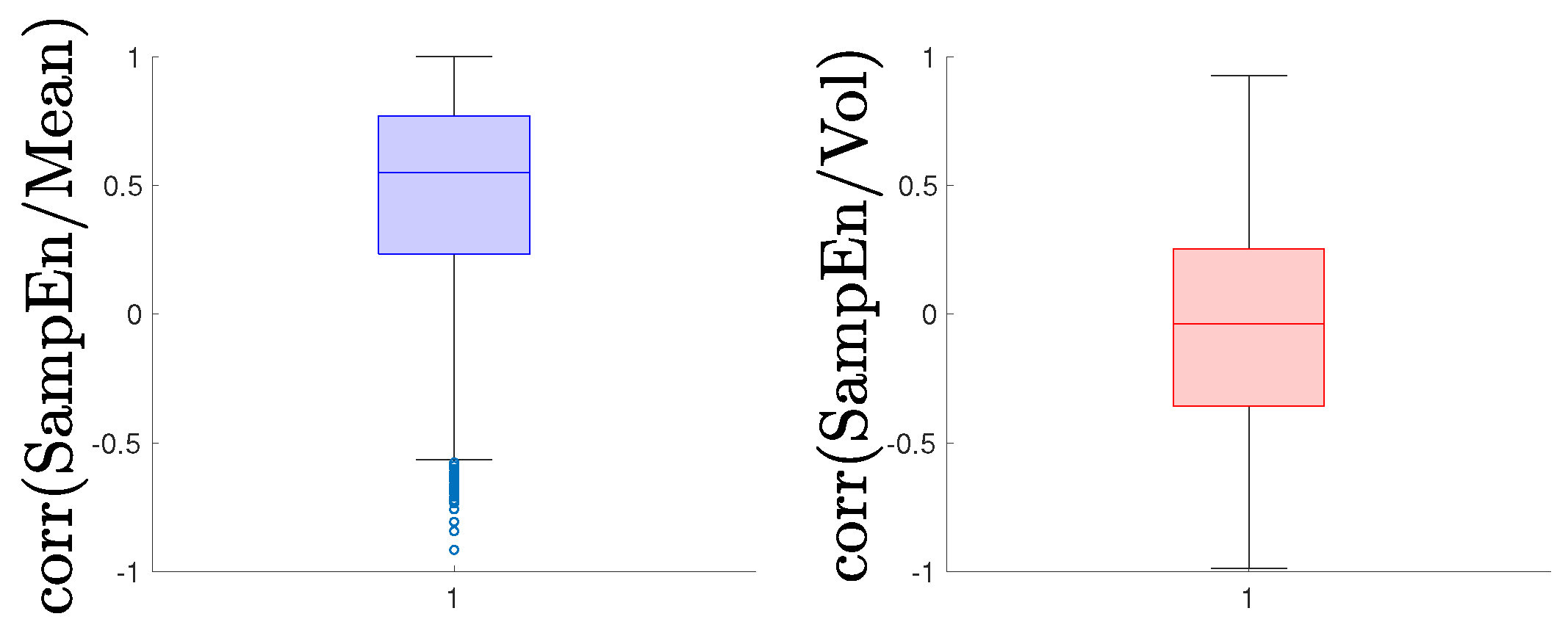
| Correlation | ||
|---|---|---|
| /Mean | /Vol. | |
| Mean | 0.4510 | −0.0509 |
| Mode | 0.7333 | 0.1152 |
| Ex. Kurtosis | 0.5456 | −0.7753 |
| Skewness | −1.0548 | −0.0626 |
Disclaimer/Publisher’s Note: The statements, opinions and data contained in all publications are solely those of the individual author(s) and contributor(s) and not of MDPI and/or the editor(s). MDPI and/or the editor(s) disclaim responsibility for any injury to people or property resulting from any ideas, methods, instructions or products referred to in the content. |
© 2023 by the authors. Licensee MDPI, Basel, Switzerland. This article is an open access article distributed under the terms and conditions of the Creative Commons Attribution (CC BY) license (https://creativecommons.org/licenses/by/4.0/).
Share and Cite
Orlando, G.; Lampart, M. Expecting the Unexpected: Entropy and Multifractal Systems in Finance. Entropy 2023, 25, 1527. https://doi.org/10.3390/e25111527
Orlando G, Lampart M. Expecting the Unexpected: Entropy and Multifractal Systems in Finance. Entropy. 2023; 25(11):1527. https://doi.org/10.3390/e25111527
Chicago/Turabian StyleOrlando, Giuseppe, and Marek Lampart. 2023. "Expecting the Unexpected: Entropy and Multifractal Systems in Finance" Entropy 25, no. 11: 1527. https://doi.org/10.3390/e25111527
APA StyleOrlando, G., & Lampart, M. (2023). Expecting the Unexpected: Entropy and Multifractal Systems in Finance. Entropy, 25(11), 1527. https://doi.org/10.3390/e25111527