

Multivariate Multiscale Cosine Similarity Entropy and Its Application to Examine Circularity Properties in Division Algebras †

Abstract
:1. Introduction
- The distance measure utilized in SampEn and FuzzyEn is based on the amplitude of the time series, where the unlimited range would lead to undefined values.
- Due to the signal related parameter setting, when the tolerance is set according to the value of standard deviation, the data normalization is required in advance, which would re-scale the original signal and cause information loss.
- Considering the requirement of re-scaling, this affects the noise robustness of SampEn and FuzzyEn, in particular, when processing short time series.
- Long data length is required for traditional SampEn and FuzzyEn analyses when exploring complexity with a high embedding dimension.
2. Related Work and Development of Existing Sample Entropy and Fuzzy Entropy
3. Multivariate Multiscale Sample Entropy and Multivariate Multiscale Fuzzy Entropy
3.1. Sample Entropy and Fuzzy Entropy
| Algorithm 1. Sample Entropy |
Given a univariate data set of length N, the parameters involved are the embedding dimension, m, tolerance, , and time delay, l.
|
| Algorithm 2. Fuzzy entropy. |
Given a univariate data set of length N, the parameters involved are the embedding dimension, m, tolerance, , and time delay, l. The fuzzy function applied here is the Gaussian function with a chosen order, .
|
3.2. Multiscale Entropy
| Algorithm 3. Multiscale sample entropy and multiscale fuzzy entropy. |
Assume that a univariate data set, , is of length, N, and the coarse graining scale factor is donated as .
|
3.3. Multivariate Multiscale Entropy
| Algorithm 4. Multivariate multiscale sample entropy and multivariate multiscale fuzzy entropy |
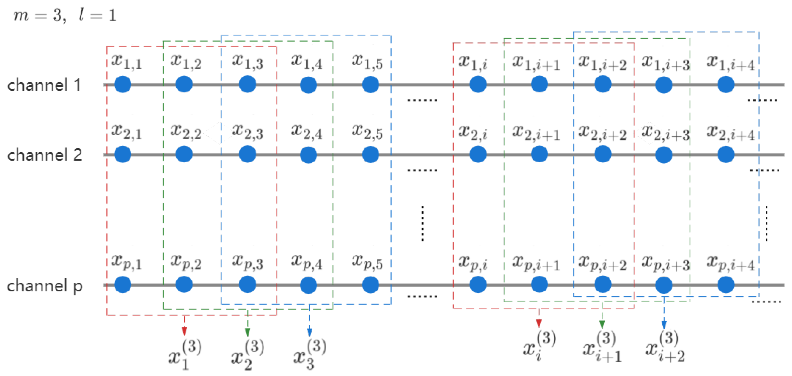
Given a multivariate data set with P channels , of length N. Parameters involved are the embedding dimension, , tolerance, r, time delay, , and the scale factor, .
|
4. Cosine Similarity Entropy and Multi-Variate Approach
| Algorithm 5. Multivariate multiscale cosine similarity entropy. |
Given a multivariate data set with P channels , of length N. Parameters involved are designated as the embedding dimension, , tolerance, , time delay, , and the scale factor, .
|
5. Value of Parameters
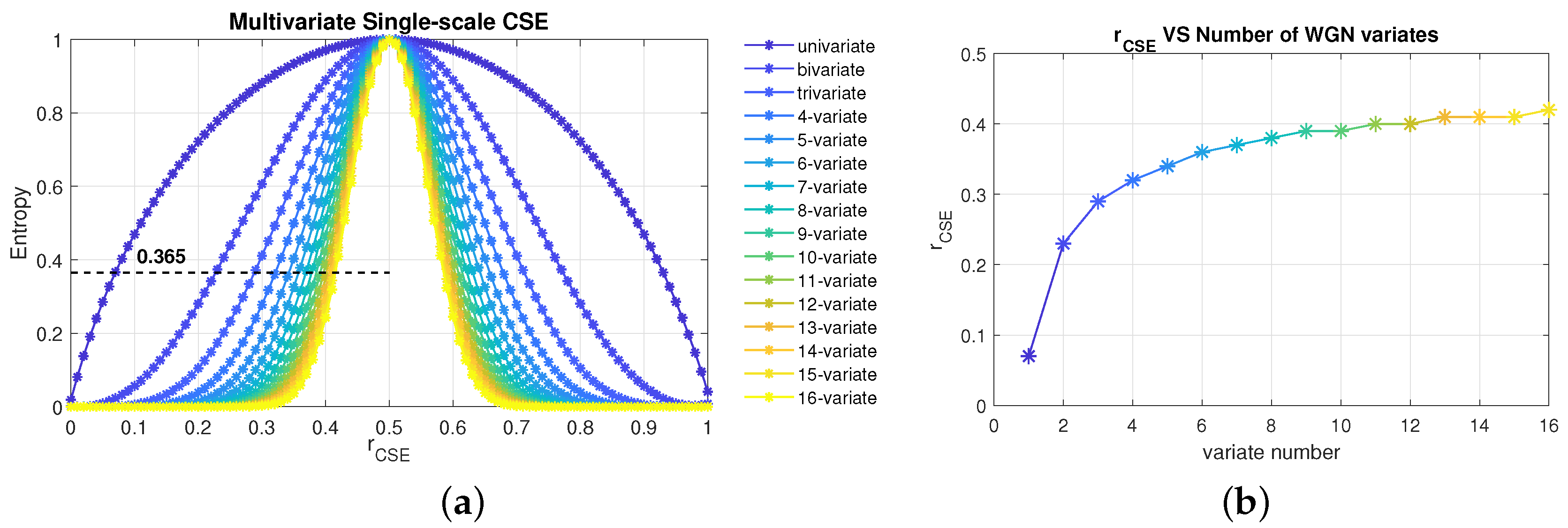
5.1. Tolerance, r
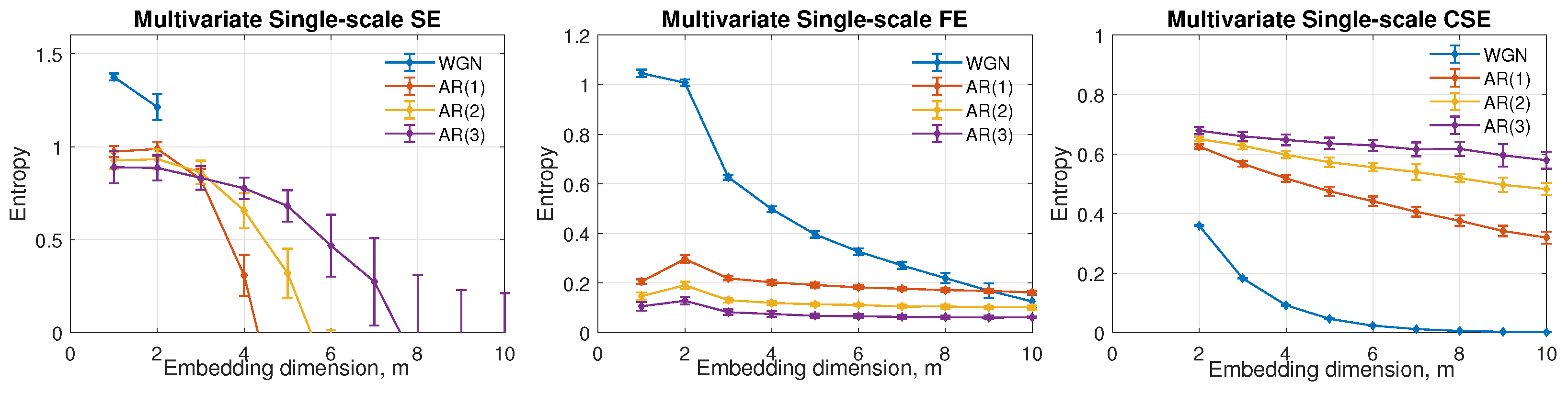
5.2. Embedding Dimension, m, and Data Length, N
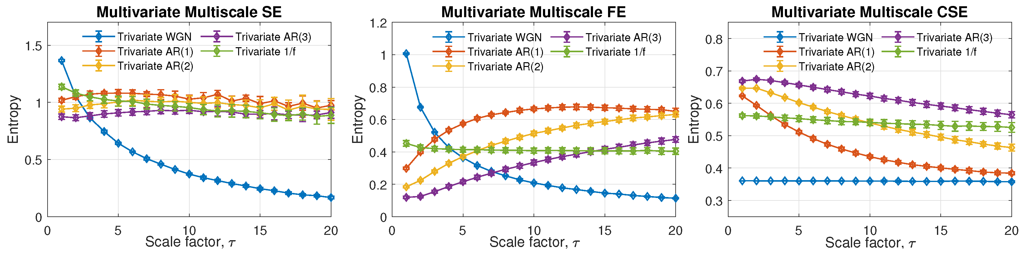
5.3. Complexity Profile of MMCSE, MMSE and MMFE
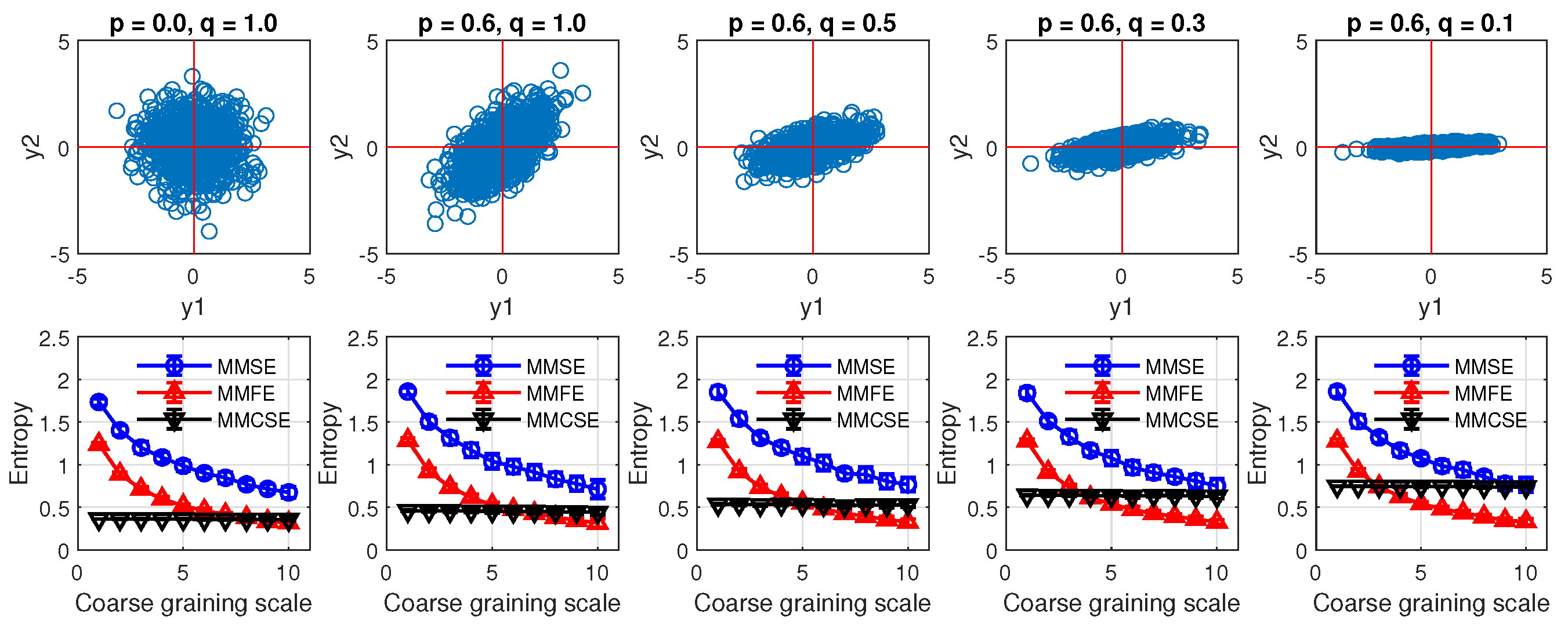
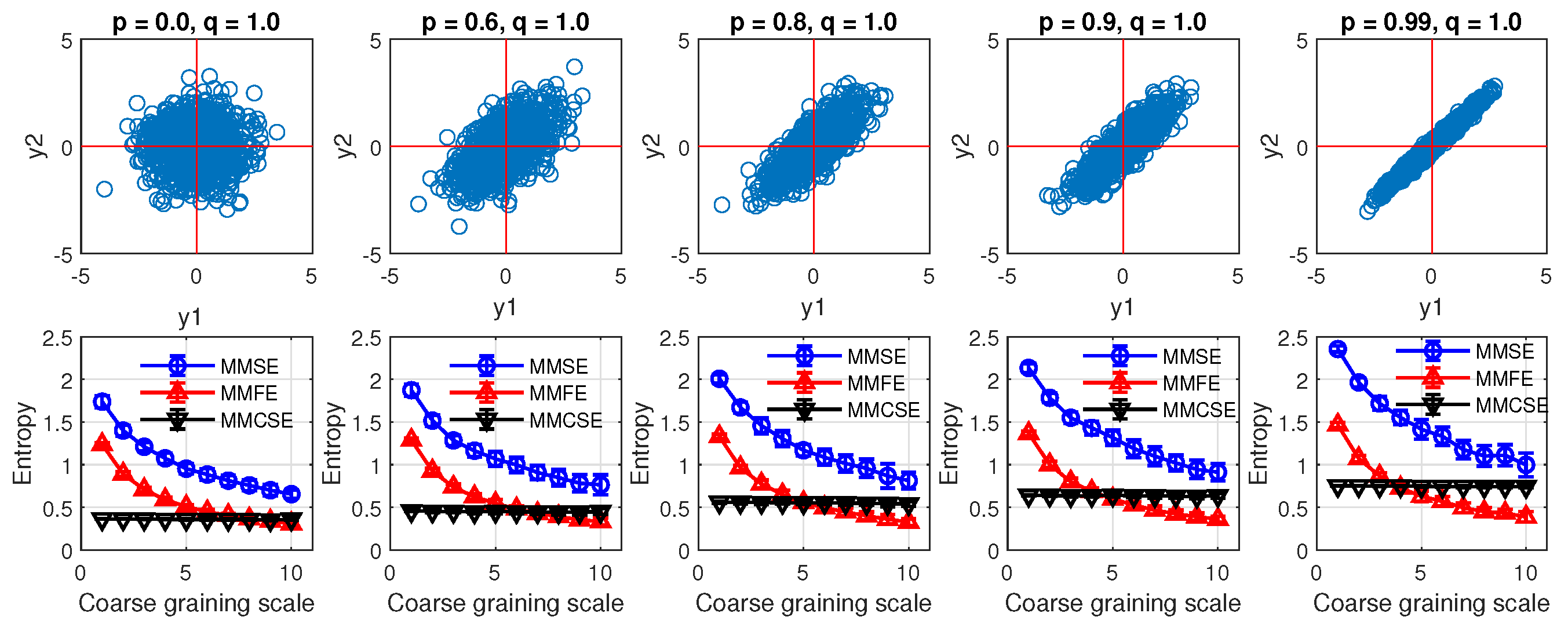
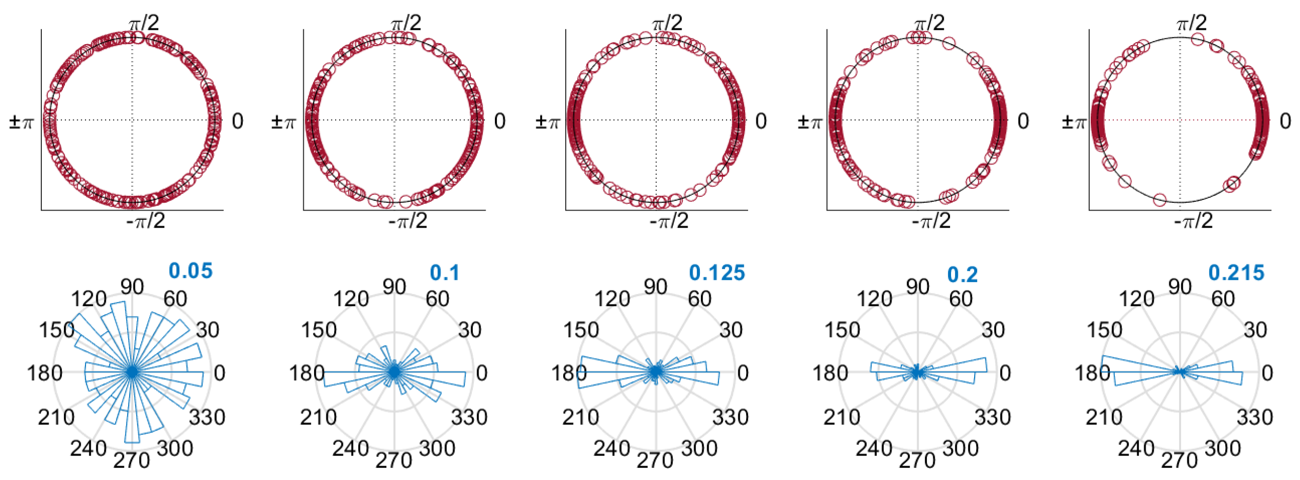
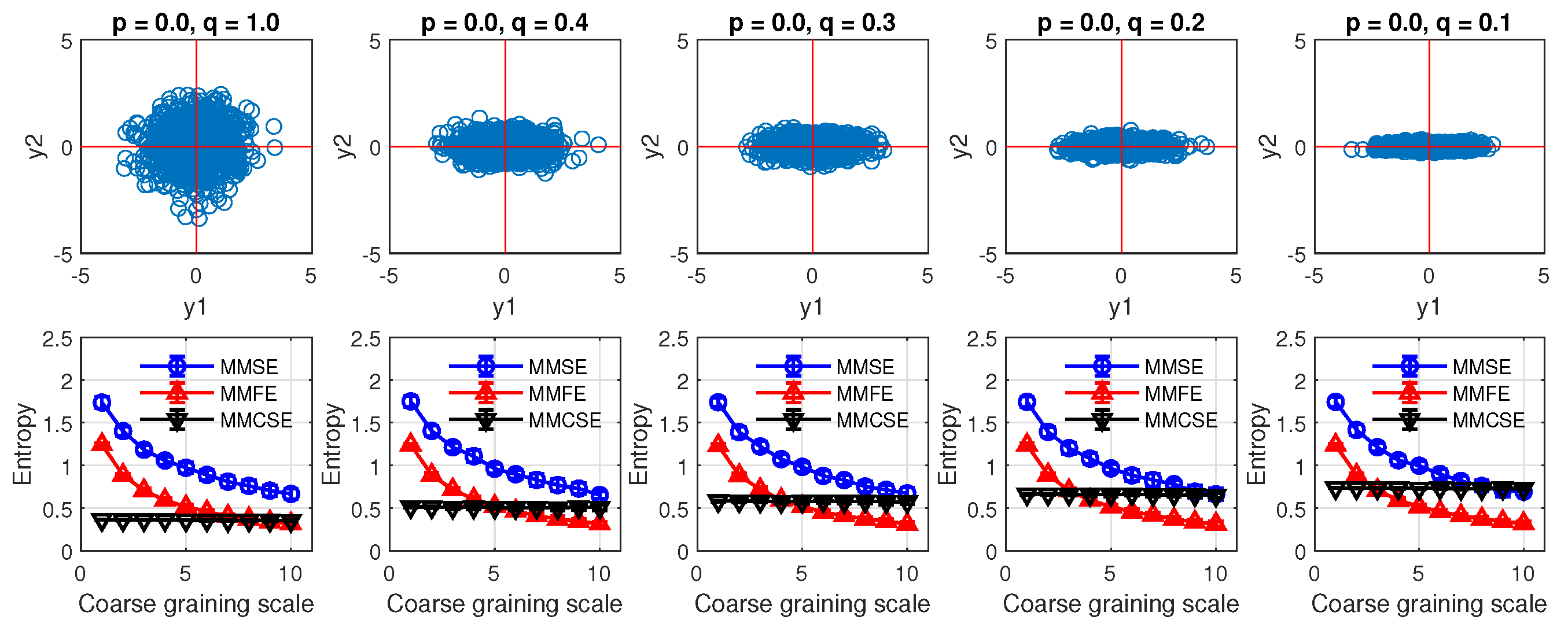
6. Detection of Circularity
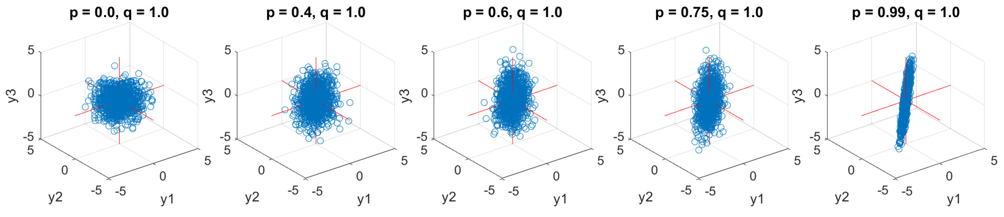
6.1. Correlated WGN with Equal Power
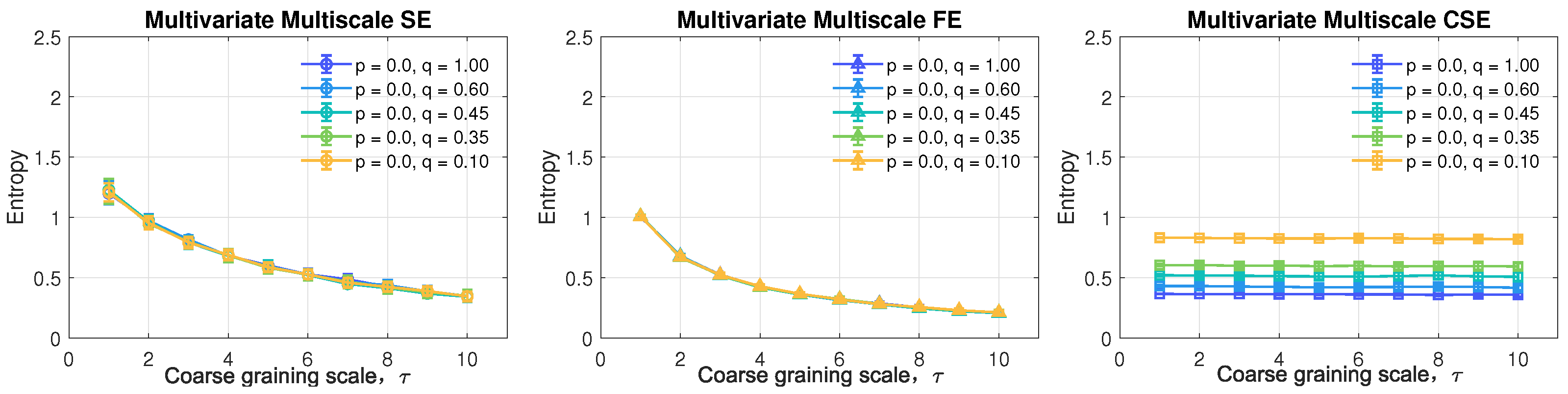
6.2. Uncorrelated WGN with Unequal Power
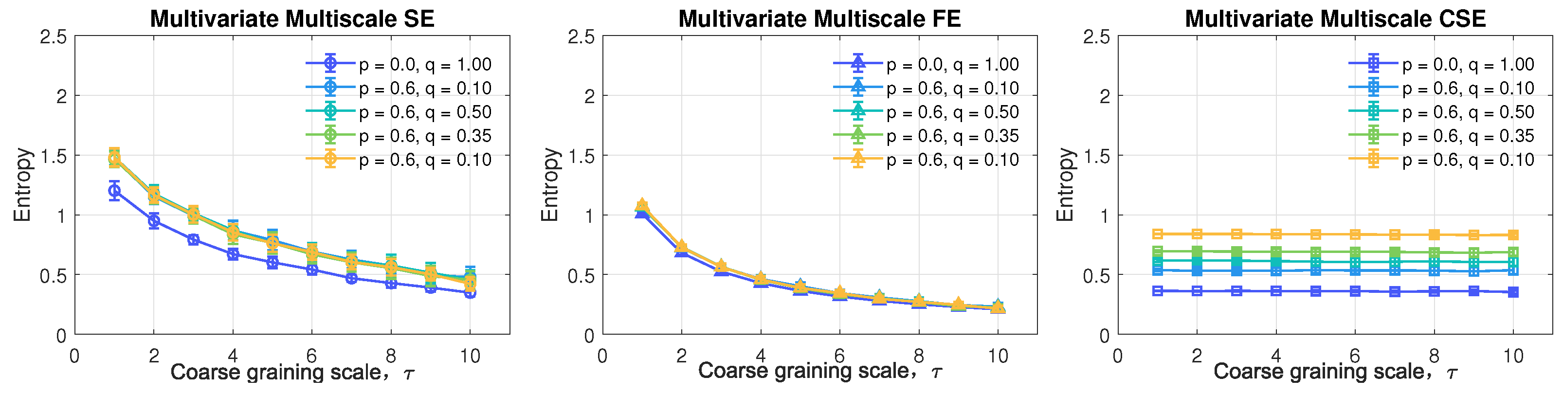
6.3. Correlated WGN with unequal power
7. Conclusions
Author Contributions
Funding
Institutional Review Board Statement
Informed Consent Statement
Data Availability Statement
Conflicts of Interest
Appendix A. Examination of Non-Circularity of Bi-Variate Systems
Appendix A.1. Correlated WGN with Equal Power


Appendix A.2. Uncorrelated WGN with Unequal Power


Appendix A.3. Correlated WGN with Unequal Power

References
- Li, Y.; Wang, X.; Liu, Z.; Liang, X.; Si, S. The entropy algorithm and its variants in the fault diagnosis of rotating machinery: A review. IEEE Access 2018, 6, 66723–66741. [Google Scholar] [CrossRef]
- Morabito, F.C.; Labate, D.; La Foresta, F.; Bramanti, A.; Morabito, G.; Palamara, I. Multivariate multi-scale permutation entropy for complexity analysis of Alzheimer’s disease EEG. Entropy 2012, 14, 1186–1202. [Google Scholar] [CrossRef]
- Marinescu, D.C. Classical and Quantum Information; Academic Press: Cambridge, MA, USA, 2011. [Google Scholar]
- Shannon, C.E. A mathematical theory of communication. Bell Syst. Tech. J. 1948, 27, 379–423. [Google Scholar] [CrossRef]
- Blahut, R.E. Principles and Practice of Information Theory; Addison-Wesley Longman Publishing Co., Inc.: Boston, MA, USA, 1987. [Google Scholar]
- Pincus, S.M. Approximate entropy as a measure of system complexity. Proc. Natl. Acad. Sci. USA 1991, 88, 2297–2301. [Google Scholar] [CrossRef]
- Richman, J.S.; Moorman, J.R. Physiological time-series analysis using approximate entropy and sample entropy. Am. J. Physiol.-Heart Circ. Physiol. 2000, 278, H2039–H2049. [Google Scholar] [CrossRef]
- Humeau-Heurtier, A.; Wu, C.W.; Wu, S.D. Refined composite multiscale permutation entropy to overcome multiscale permutation entropy length dependence. IEEE Signal Process. Lett. 2015, 22, 2364–2367. [Google Scholar] [CrossRef]
- Ni, L.; Cao, J.; Wang, R. Analyzing EEG of quasi-brain-death based on dynamic sample entropy measures. Comput. Math. Methods Med. 2013, 2013, 618743. [Google Scholar] [CrossRef]
- Govindan, R.; Wilson, J.; Eswaran, H.; Lowery, C.; Preißl, H. Revisiting sample entropy analysis. Phys. A Stat. Mech. Its Appl. 2007, 376, 158–164. [Google Scholar] [CrossRef]
- Looney, D.; Adjei, T.; Mandic, D.P. A novel multivariate sample entropy algorithm for modeling time series synchronization. Entropy 2018, 20, 82. [Google Scholar] [CrossRef]
- Xiao, H.; Mandic, D.P. Variational embedding multiscale sample entropy: A tool for complexity analysis of multichannel systems. Entropy 2021, 24, 26. [Google Scholar] [CrossRef]
- Hemakom, A.; Goverdovsky, V.; Looney, D.; Mandic, D.P. Adaptive-projection intrinsically transformed multivariate empirical mode decomposition in cooperative brain–computer interface applications. Philos. Trans. R. Soc. A Math. Phys. Eng. Sci. 2016, 374, 20150199. [Google Scholar] [CrossRef] [PubMed]
- Alcaraz, R.; Abásolo, D.; Hornero, R.; Rieta, J. Study of Sample Entropy ideal computational parameters in the estimation of atrial fibrillation organization from the ECG. In Proceedings of the IEEE Conference on Computing in Cardiology, Belfast, UK, 26–29 September 2010; pp. 1027–1030. [Google Scholar]
- Chanwimalueang, T.; Aufegger, L.; von Rosenberg, W.; Mandic, D.P. Modelling stress in public speaking: Evolution of stress levels during conference presentations. In Proceedings of the IEEE International Conference on Acoustics, Speech and Signal Processing (ICASSP), Shanghai, China, 20–25 March 2016; pp. 814–818. [Google Scholar]
- Chen, W.; Wang, Z.; Xie, H.; Yu, W. Characterization of surface EMG signal based on fuzzy entropy. IEEE Trans. Neural Syst. Rehabil. Eng. 2007, 15, 266–272. [Google Scholar] [CrossRef] [PubMed]
- Bradley, M.M.; Miccoli, L.; Escrig, M.A.; Lang, P.J. The pupil as a measure of emotional arousal and autonomic activation. Psychophysiology 2008, 45, 602–607. [Google Scholar] [CrossRef]
- Chanwimalueang, T.; Mandic, D.P. Cosine Similarity Entropy: Self-Correlation-Based Complexity Analysis of Dynamical Systems. Entropy 2017, 19, 652. [Google Scholar] [CrossRef]
- Ahmed, M.U.; Mandic, D.P. Multivariate multiscale entropy: A tool for complexity analysis of multichannel data. Phys. Rev. E 2011, 84, 061918. [Google Scholar] [CrossRef] [PubMed]
- Costa, M.; Goldberger, A.L.; Peng, C.K. Multiscale entropy analysis of complex physiologic time series. Phys. Rev. Lett. 2002, 89, 068102. [Google Scholar] [CrossRef] [PubMed]
- Valencia, J.F.; Porta, A.; Vallverdu, M.; Claria, F.; Baranowski, R.; Orlowska-Baranowska, E.; Caminal, P. Refined multiscale entropy: Application to 24-h holter recordings of heart period variability in healthy and aortic stenosis subjects. IEEE Trans. Biomed. Eng. 2009, 56, 2202–2213. [Google Scholar] [CrossRef]
- Ahmed, M.; Rehman, N.; Looney, D.; Rutkowski, T.; Mandic, D. Dynamical complexity of human responses: A multivariate data-adaptive framework. Bull. Pol. Acad. Sci. Tech. Sci. 2012, 60, 433–445. [Google Scholar] [CrossRef]
- Wu, S.D.; Wu, C.W.; Lin, S.G.; Wang, C.C.; Lee, K.Y. Time series analysis using composite multiscale entropy. Entropy 2013, 15, 1069–1084. [Google Scholar] [CrossRef]
- Costa, M.D.; Goldberger, A.L. Generalized multiscale entropy analysis: Application to quantifying the complex volatility of human heartbeat time series. Entropy 2015, 17, 1197–1203. [Google Scholar] [CrossRef]
- Amoud, H.; Snoussi, H.; Hewson, D.; Doussot, M.; Duchene, J. Intrinsic mode entropy for nonlinear discriminant analysis. IEEE Signal Process. Lett. 2007, 14, 297–300. [Google Scholar] [CrossRef]
- Ahmed, M.U.; Chanwimalueang, T.; Thayyil, S.; Mandic, D.P. A multivariate multiscale fuzzy entropy algorithm with application to uterine EMG complexity analysis. Entropy 2017, 19, 2. [Google Scholar] [CrossRef]
- Costa, M.D.; Peng, C.K.; Goldberger, A.L. Multiscale analysis of heart rate dynamics: Entropy and time irreversibility measures. Cardiovasc. Eng. 2008, 8, 88–93. [Google Scholar] [CrossRef] [PubMed]
- Takens, F. Detecting strange attractors in turbulence. In Dynamical Systems and Turbulence, Warwick 1980; Springer: Berlin/Heidelberg, Germany, 1981; pp. 366–381. [Google Scholar]
- Hausdorff, J.M. Gait dynamics in Parkinson’s disease: Common and distinct behavior among stride length, gait variability, and fractal-like scaling. Chaos Interdiscip. J. Nonlinear Sci. 2009, 19, 026113. [Google Scholar] [CrossRef] [PubMed]
- Gautama, T.; Mandic, D.P.; Van Hulle, M.M. A differential entropy based method for determining the optimal embedding parameters of a signal. In Proceedings of the 2003 IEEE International Conference on Acoustics, Speech, and Signal Processing (ICASSP’03), Hong Kong, China, 6–10 April 2003; Volume 6, p. VI-29. [Google Scholar]
- Menayo, R.; Manzanares, A.; Segado, F. Complexity, Regularity and Non-Linear Behavior in Human Eye Movements: Analyzing the Dynamics of Gaze in Virtual Sailing Programs. Symmetry 2018, 10, 528. [Google Scholar] [CrossRef]
- Pincus, S. Approximate entropy as an irregularity measure for financial data. Econom. Rev. 2008, 27, 329–362. [Google Scholar] [CrossRef]
- Paluš, M. Testing for nonlinearity using redundancies: Quantitative and qualitative aspects. Phys. D Nonlinear Phenom. 1995, 80, 186–205. [Google Scholar] [CrossRef]
- Malik, M.; Bigger, J.T.; Camm, A.J.; Kleiger, R.E.; Malliani, A.; Moss, A.J.; Schwartz, P.J. Heart rate variability: Standards of measurement, physiological interpretation, and clinical use. Eur. Heart J. 1996, 17, 354–381. [Google Scholar] [CrossRef]
- von Rosenberg, W.; Chanwimalueang, T.; Adjei, T.; Jaffer, U.; Goverdovsky, V.; Mandic, D.P. Resolving ambiguities in the LF/HF ratio: LF-HF scatter plots for the categorization of mental and physical stress from HRV. Front. Physiol. 2017, 8, 360. [Google Scholar] [CrossRef]
- Berens, P. CircStat: A MATLAB toolbox for circular statistics. J. Stat. Softw. 2009, 31, 1–21. [Google Scholar] [CrossRef] [Green Version]


| Coefficients | |||
|---|---|---|---|
| AR | − | − | |
| AR | − | ||
| AR |
Publisher’s Note: MDPI stays neutral with regard to jurisdictional claims in published maps and institutional affiliations. |
© 2022 by the authors. Licensee MDPI, Basel, Switzerland. This article is an open access article distributed under the terms and conditions of the Creative Commons Attribution (CC BY) license (https://creativecommons.org/licenses/by/4.0/).
Share and Cite
Xiao, H.; Chanwimalueang, T.; Mandic, D.P. Multivariate Multiscale Cosine Similarity Entropy and Its Application to Examine Circularity Properties in Division Algebras. Entropy 2022, 24, 1287. https://doi.org/10.3390/e24091287
Xiao H, Chanwimalueang T, Mandic DP. Multivariate Multiscale Cosine Similarity Entropy and Its Application to Examine Circularity Properties in Division Algebras. Entropy. 2022; 24(9):1287. https://doi.org/10.3390/e24091287
Chicago/Turabian StyleXiao, Hongjian, Theerasak Chanwimalueang, and Danilo P. Mandic. 2022. "Multivariate Multiscale Cosine Similarity Entropy and Its Application to Examine Circularity Properties in Division Algebras" Entropy 24, no. 9: 1287. https://doi.org/10.3390/e24091287
APA StyleXiao, H., Chanwimalueang, T., & Mandic, D. P. (2022). Multivariate Multiscale Cosine Similarity Entropy and Its Application to Examine Circularity Properties in Division Algebras. Entropy, 24(9), 1287. https://doi.org/10.3390/e24091287