
Deep Sparse Autoencoder and Recursive Neural Network for EEG Emotion Recognition


Abstract
:1. Introduction
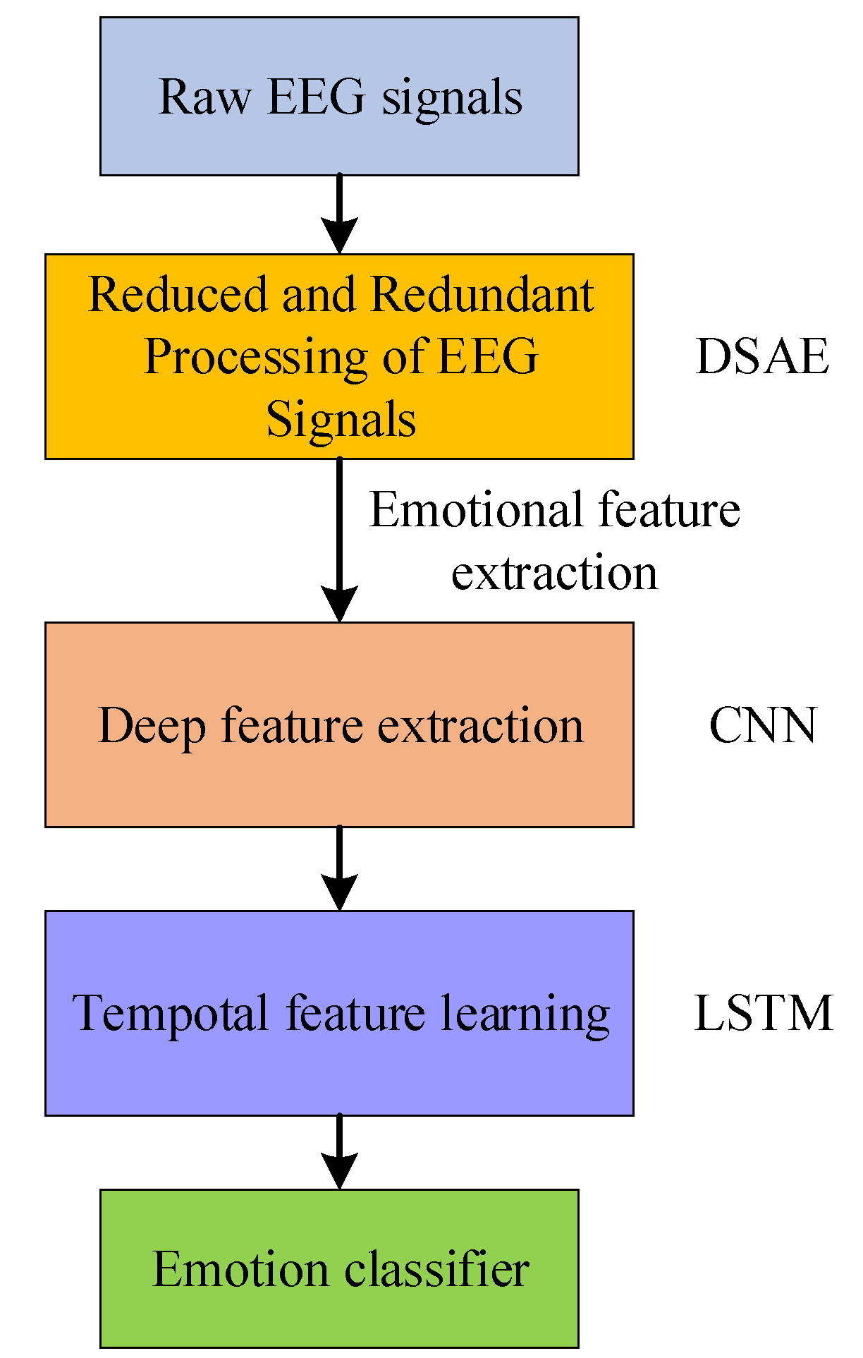
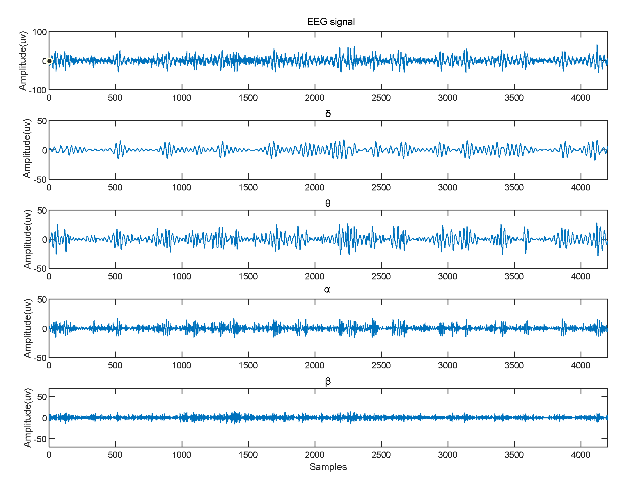
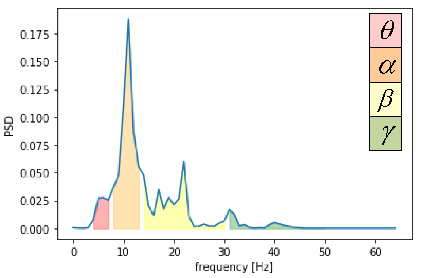
2. Methods
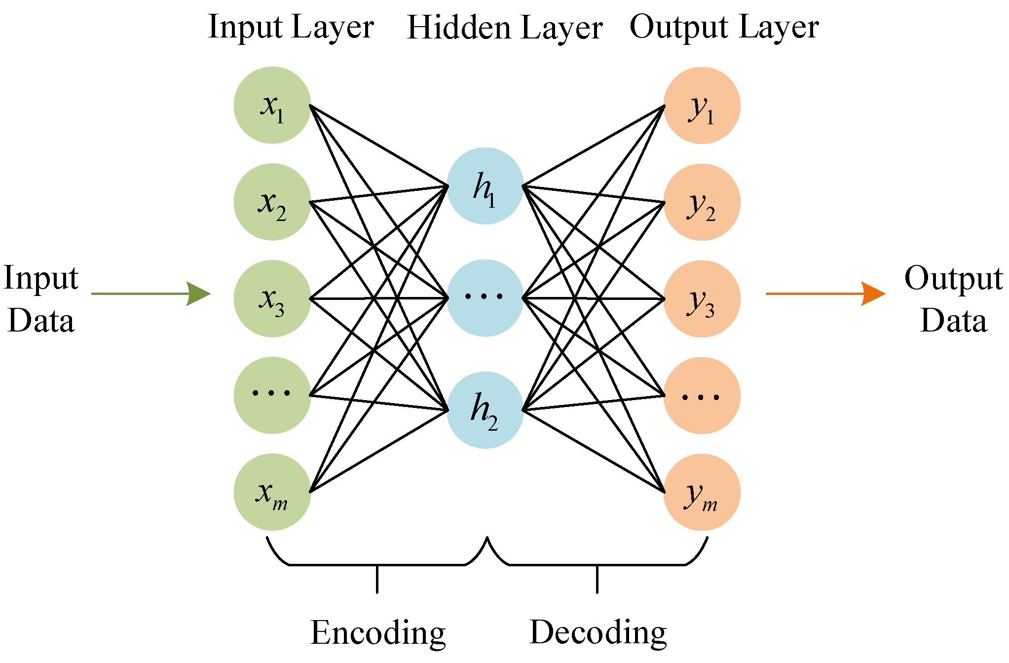
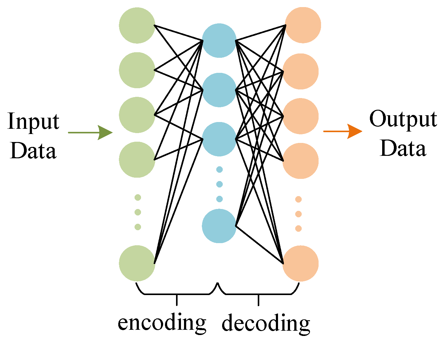
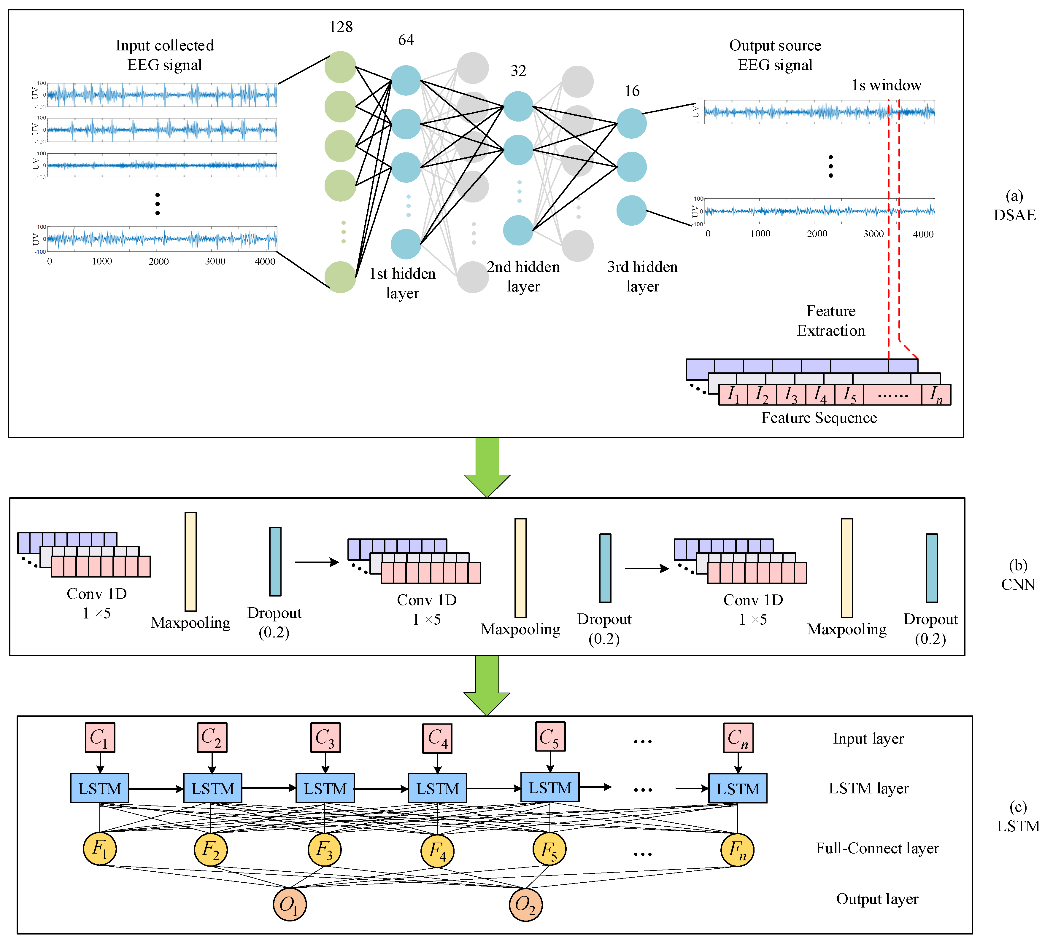
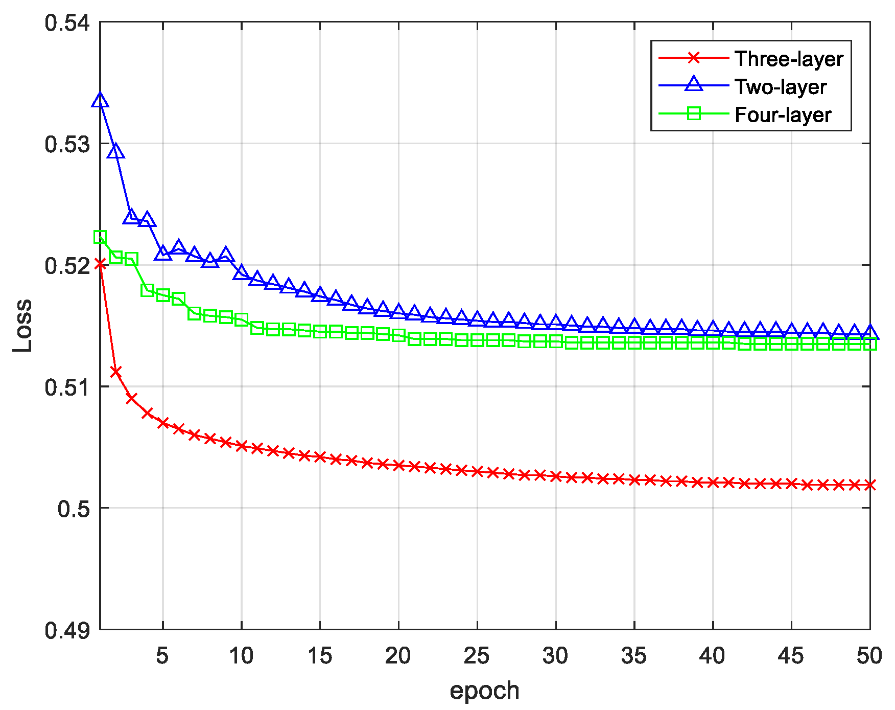
2.1. Sparse Autoencoder (SAE)
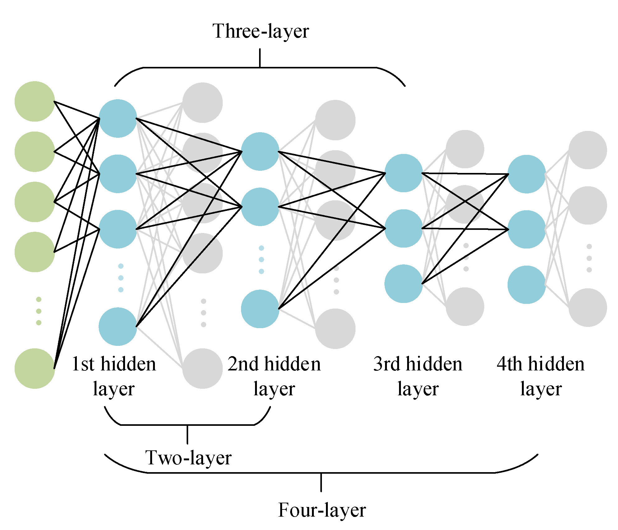
2.2. Hybrid Neural Network Methods
3. Experiments and Results
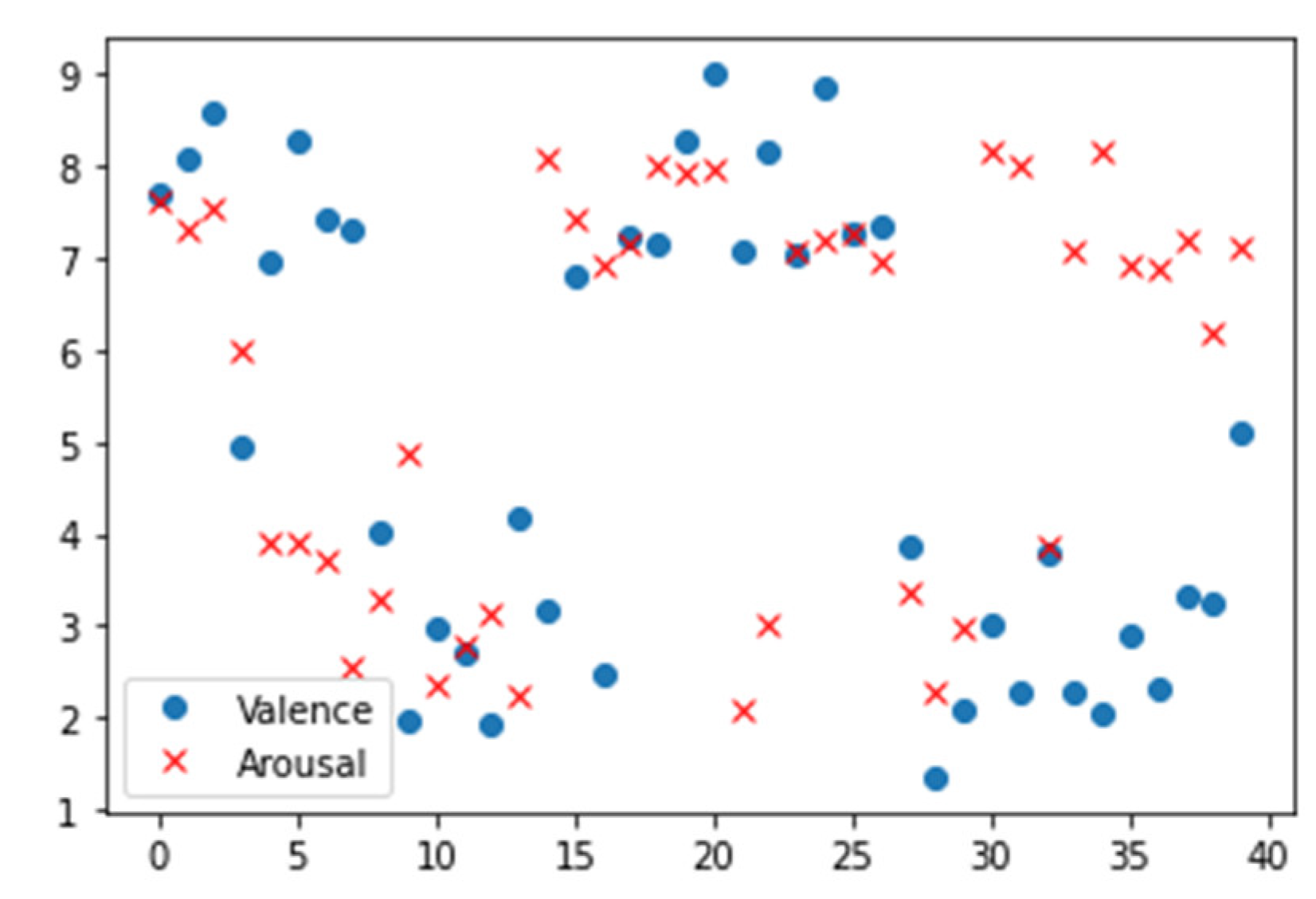
3.1. Datasets and Emotion Label Processing
3.2. Experiment Setup
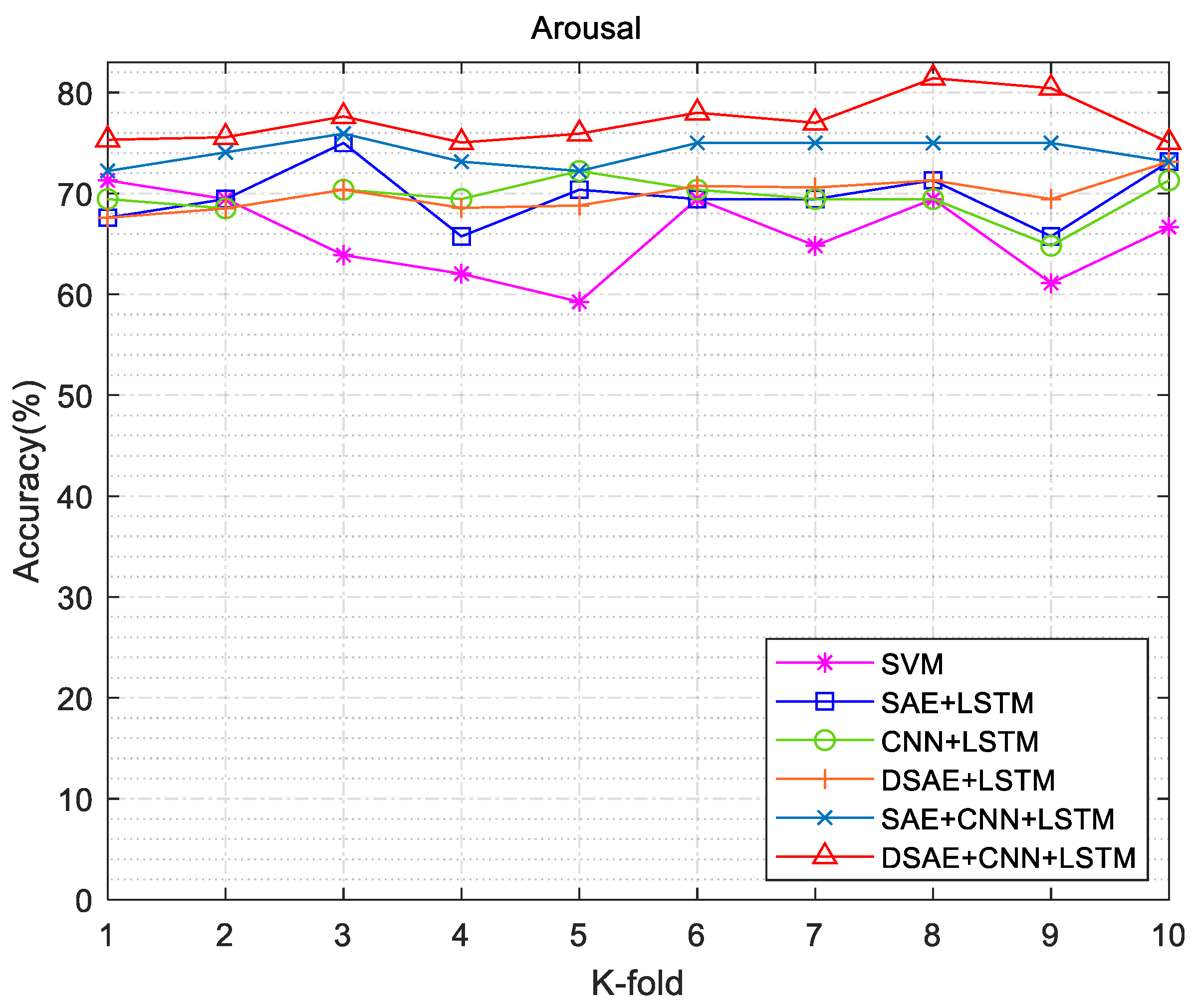
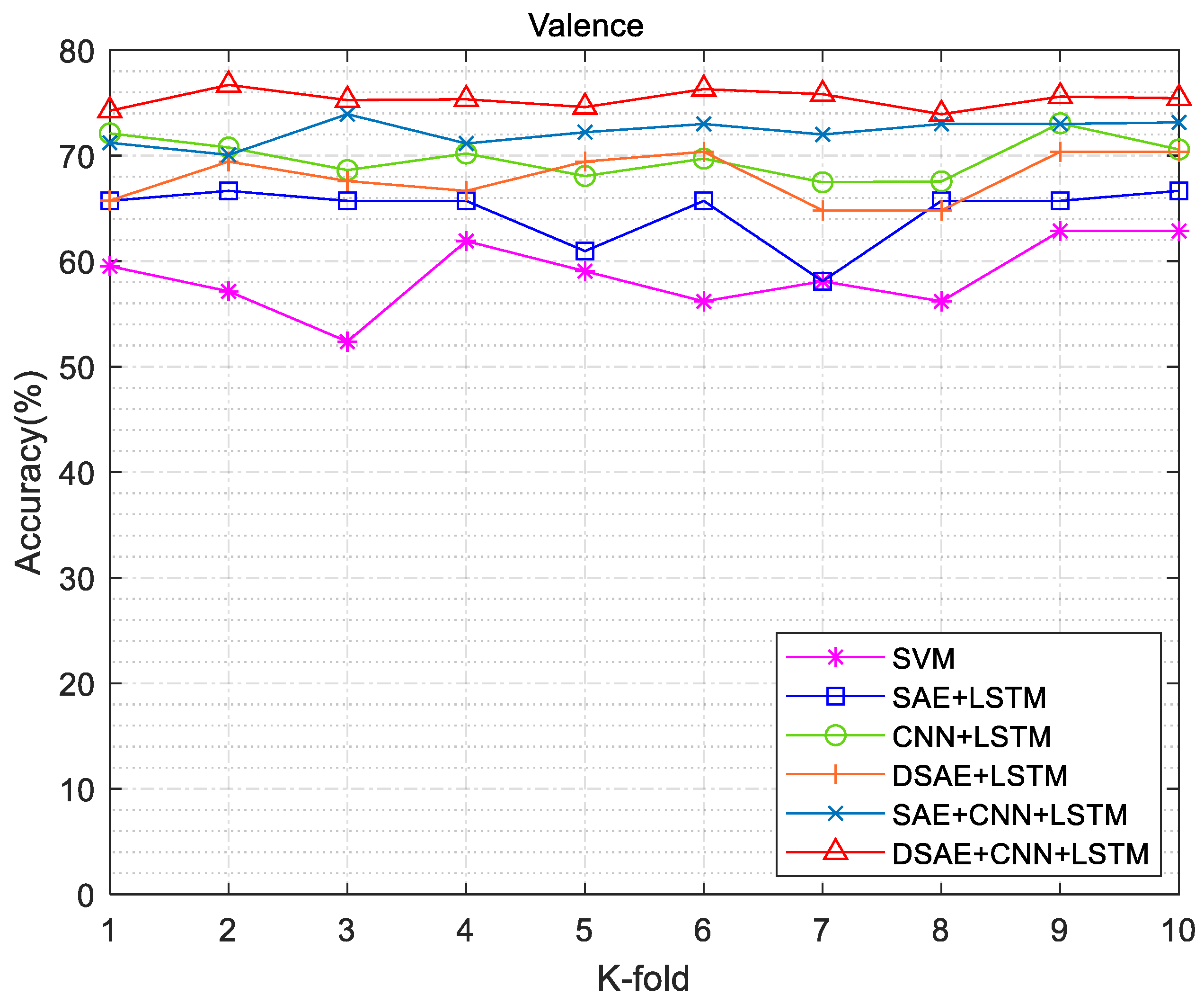
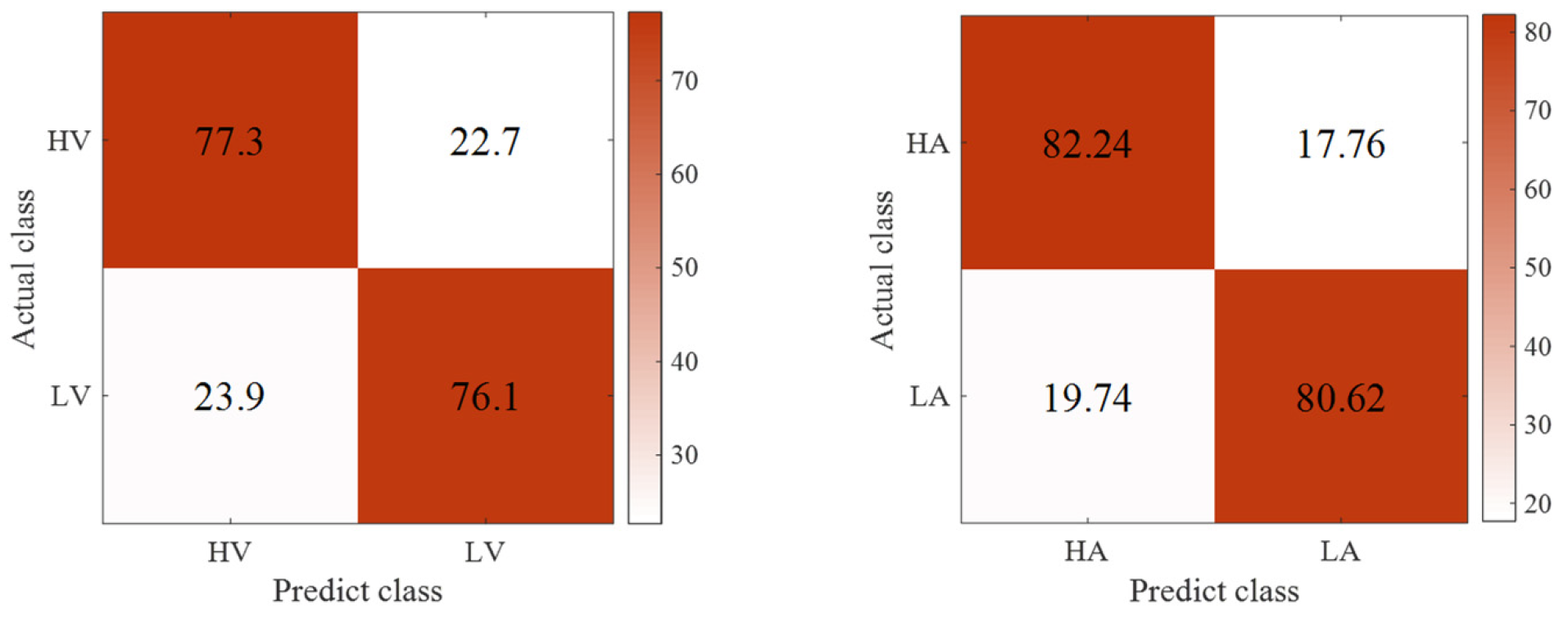
3.3. Emotion Recognition Results
4. Conclusions
Author Contributions
Funding
Informed Consent Statement
Data Availability Statement
Conflicts of Interest
References
- Luo, J.; Tian, Y.; Yu, H.; Chen, Y.; Wu, M. Semi-Supervised Cross-Subject Emotion Recognition Based on Stacked Denoising Autoencoder Architecture Using a Fusion of Multi-Modal Physiological Signals. Entropy 2022, 24, 577. [Google Scholar] [CrossRef] [PubMed]
- García-Martínez, B.; Martínez-Rodrigo, A.; Zangróniz Cantabrana, R.; Pastor Garcia, J.M.; Alcaraz, R. Application of entropy-based metrics to identify emotional distress from electroencephalographic recordings. Entropy 2016, 18, 221. [Google Scholar] [CrossRef]
- Yang, H.; Huang, S.; Guo, S.; Sun, G. Multi-Classifier Fusion Based on MI–SFFS for Cross-Subject Emotion Recognition. Entropy 2022, 24, 705. [Google Scholar] [CrossRef] [PubMed]
- Yao, L.; Wang, M.; Lu, Y.; Li, H.; Zhang, X. EEG-based emotion recognition by exploiting fused network entropy measures of complex networks across subjects. Entropy 2021, 23, 984. [Google Scholar] [CrossRef] [PubMed]
- Guastello, S.J. Physiological synchronization in a vigilance dual task. Nonlinear dynamics, psychology, and life sciences. Nonlinear Dyn. Psychol. Life Sci. 2016, 20, 49–80. [Google Scholar]
- Nguyen, T.; Hettiarachchi, I.; Khatami, A.; Gordon-Brown, L.; Lim, C.P.; Nahavandi, S. Classification of multi-class BCI data by common spatial pattern and fuzzy system. IEEE Access 2018, 6, 27873–27884. [Google Scholar] [CrossRef]
- Veerabhadrappa, R.; Ul Hassan, M.; Zhang, J.; Bhatti, A. Compatibility evaluation of clustering algorithms for contemporary extracellular neural spike sorting. Front. Syst. Neurosci. 2020, 14, 34. [Google Scholar] [CrossRef]
- Libert, A.; Van Hulle, M.M. Predicting premature video skipping and viewer interest from EEG recordings. Entropy 2019, 21, 1014. [Google Scholar] [CrossRef]
- Kumar, N.; Khaund, K.; Hazarika, S.M. Bispectral analysis of EEG for emotion recognition. Procedia Comput. Sci. 2016, 84, 31–35. [Google Scholar] [CrossRef]
- Wang, Y.; Qiu, S.; Li, J.; Ma, X.; Liang, Z.; Li, H.; He, H. EEG-based emotion recognition with similarity learning network. In Proceedings of the 2019 41st Annual International Conference of the IEEE Engineering in Medicine and Biology Society (EMBC), Berlin, Germany, 23–27 July 2019; pp. 1209–1212. [Google Scholar]
- Zheng, W.L.; Liu, W.; Lu, Y.; Lu, B.L.; Cichocki, A. Emotionmeter: A multimodal framework for recognizing human emotions. IEEE Trans. Cybern. 2018, 49, 1110–1122. [Google Scholar] [CrossRef]
- Atkinson, J.; Campos, D. Improving BCI-based emotion recognition by combining EEG feature selection and kernel classifiers. Expert Syst. Appl. 2016, 47, 35–41. [Google Scholar] [CrossRef]
- Islam, M.R.; Moni, M.A.; Islam, M.M.; Rashed-Al-Mahfuz, M.; Islam, M.S.; Hasan, M.K.; Lió, P. Emotion recognition from EEG signal focusing on deep learning and shallow learning techniques. IEEE Access 2021, 9, 94601–94624. [Google Scholar] [CrossRef]
- Islam, M.R.; Islam, M.M.; Rahman, M.M.; Mondal, C.; Singha, S.K.; Ahmad, M.; Moni, M.A. EEG channel correlation based model for emotion recognition. Comput. Biol. Med. 2021, 136, 104757. [Google Scholar] [CrossRef] [PubMed]
- Jirayucharoensak, S.; Pan-Ngum, S.; Israsena, P. EEG-based emotion recognition using deep learning network with principal component based covariate shift adaptation. Sci. World J. 2014, 2014, 627892. [Google Scholar] [CrossRef]
- Li, Y.; Huang, J.; Zhou, H.; Zhong, N. Human emotion recognition with electroencephalographic multidimensional features by hybrid deep neural networks. Appl. Sci. 2017, 7, 1060. [Google Scholar] [CrossRef]
- Zhang, Q.; Chen, X.; Zhan, Q.; Yang, T.; Xia, S. Respiration-based emotion recognition with deep learning. Comput. Ind. 2017, 92, 84–90. [Google Scholar] [CrossRef]
- Xing, X.; Li, Z.; Xu, T.; Shu, L.; Hu, B.; Xu, X. SAE+ LSTM: A New framework for emotion recognition from multi-channel EEG. Front. Neurorobot. 2019, 13, 37. [Google Scholar] [CrossRef]
- Li, J.; Struzik, Z.; Zhang, L.; Cichocki, A. Feature learning from incomplete EEG with denoising autoencoder. Neurocomputing 2015, 165, 23–31. [Google Scholar] [CrossRef]
- Rooney, I.M.; Buck, J.R. Spatial power spectral density estimation using a welch coprime sensor array processor. J. Acoust. Soc. Am. 2019, 145, 2350–2362. [Google Scholar] [CrossRef]
- Soleymani, M.; Asghari-Esfeden, S.; Fu, Y.; Pantic, M. Analysis of EEG signals and facial expressions for continuous emotion detection. IEEE Trans. Affect. Comput. 2015, 7, 17–28. [Google Scholar] [CrossRef]
- Koelstra, S.; Muhl, C.; Soleymani, M.; Lee, J.S.; Yazdani, A.; Ebrahimi, T.; Patras, I. Deap: A database for emotion analysis; using physiological signals. IEEE Trans. Affect. Comput. 2011, 3, 18–31. [Google Scholar] [CrossRef] [Green Version]
- Li, Z.; Tian, X.; Shu, L.; Xu, X.; Hu, B. Emotion recognition from EEG using RASM and LSTM. In Proceedings of the International Conference on Internet Multimedia Computing and Service, Tsingtao, China, 23–25 August 2017; Springer: Singapore, 2017; pp. 310–318. [Google Scholar]
- Ding, Y.; Robinson, N.; Zhang, S.; Zeng, Q.; Guan, C. Tsception: Capturing temporal dynamics and spatial asymmetry from EEG for emotion recognition. arXiv 2021, arXiv:2104.02935. [Google Scholar] [CrossRef]
- Ullah, H.; Uzair, M.; Mahmood, A.; Ullah, M.; Khan, S.D.; Cheikh, F.A. Internal emotion classification using EEG signal with sparse discriminative ensemble. IEEE Access 2019, 7, 40144–40153. [Google Scholar] [CrossRef]
- Li, X.; Song, D.; Zhang, P.; Yu, G.; Hou, Y.; Hu, B. Emotion recognition from multi-channel EEG data through convolutional recurrent neural network. In Proceedings of the 2016 IEEE International Conference on Bioinformatics and Biomedicine (BIBM), Shenzhen, China, 15–18 December 2016; pp. 352–359. [Google Scholar]


| Name | Size | Contents |
|---|---|---|
| Data | 40 × 40 × 8064 | video × channel × data |
| Labels | 40 × 4 | video × label (valence, arousal, dominance, liking) |
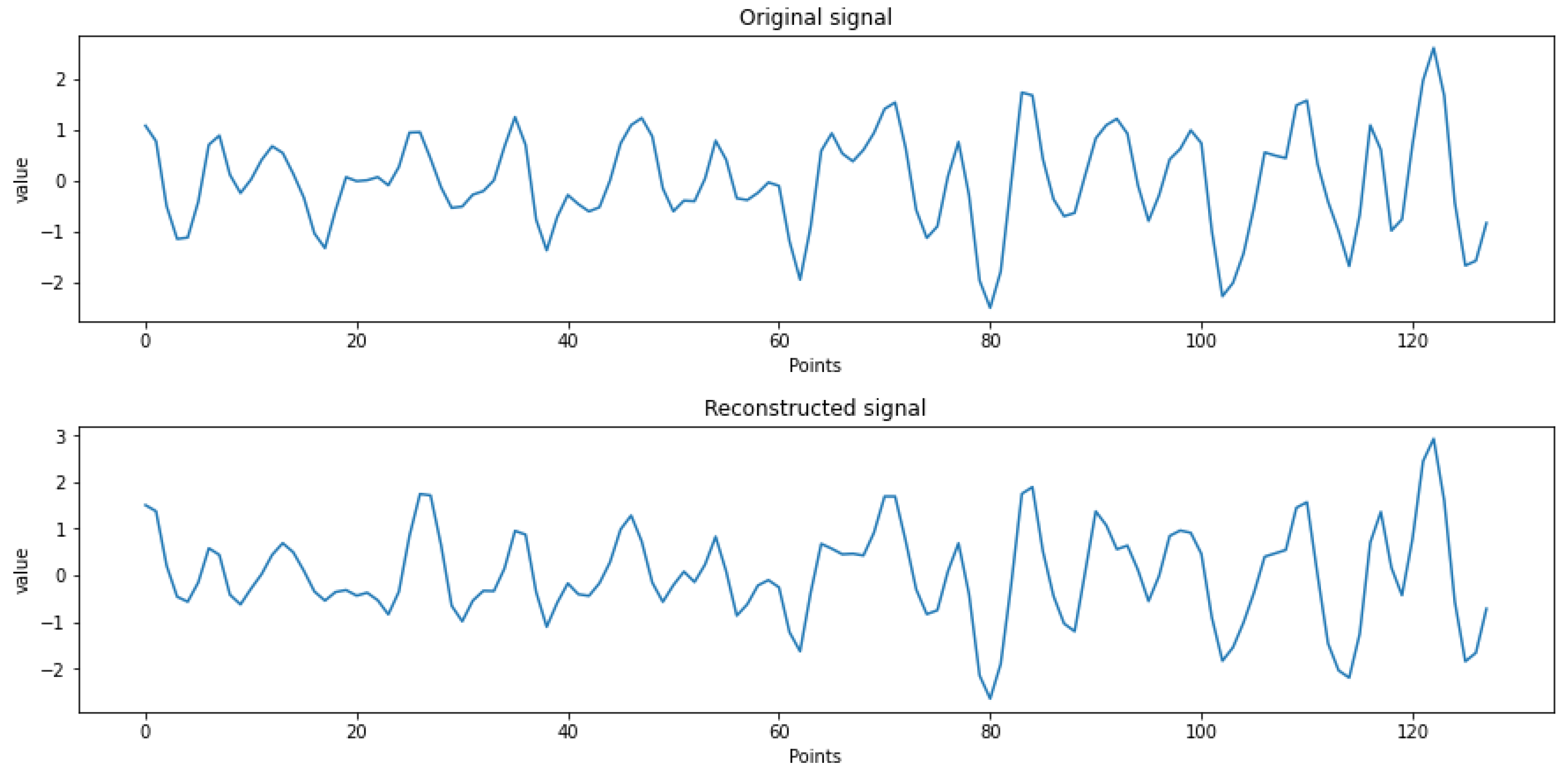
| Signals | MSE | SNR |
|---|---|---|
| Original signal | 0.020 | 32.16 |
| Reconstructed signal | 0.018 | 31.05 |
| Base Model | Combined Validation Model | Accuracy (%) | Kappa | ||
|---|---|---|---|---|---|
| Arousal | Valence | ||||
| SVM | - | 71.30 | 62.90 | 0.66 | 0.16 |
| Without SAE | CNN + LSTM | 72.23 | 73.07 | 0.67 | 0.27 |
| SAE | SAE + LSTM | 75 | 66.67 | 0.72 | 0.18 |
| SAE + CNN + LSTM | 75.93 | 73.15 | 0.79 | 0.12 | |
| DSAE | DSAE + LSTM | 73.14 | 70.37 | 0.76 | 0.08 |
| DSAE + CNN + LSTM | 81.43 | 76.70 | 0.93 | 0.05 | |
| Valence/Arousal | Class | Precision (%) | Sensitive (%) | Specificity (%) |
|---|---|---|---|---|
| Valence | High | 79.2 | 73.1 | 76.2 |
| Low | 74.0 | 79.5 | 74.9 | |
| Arousal | High | 84.7 | 78.7 | 77.9 |
| Low | 79.6 | 85.3 | 78.5 |
| Classification Methods | Features | Arousal (%) | Valence (%) | Time Cost (s) | Parameters |
|---|---|---|---|---|---|
| Ding et al. [24] | Temporal dynamics + spatial asymmetry | 61.57 | 59.14 | 1360 | 41,654 |
| Ullah et al. [25] | PCA | 70.10 | 77.40 | 753 | 12,563 |
| Li et al. [26] | CWT | 74.12 | 72.60 | 630 | 10,056 |
| Xing et al. [18] | FBP | 74.38 | 81.10 | 300 | 9443 |
| DSAE + CNN + LSTM (DCRNN) | PSD | 81.43 | 76.70 | 260 | 8384 |
Publisher’s Note: MDPI stays neutral with regard to jurisdictional claims in published maps and institutional affiliations. |
© 2022 by the authors. Licensee MDPI, Basel, Switzerland. This article is an open access article distributed under the terms and conditions of the Creative Commons Attribution (CC BY) license (https://creativecommons.org/licenses/by/4.0/).
Share and Cite
Li, Q.; Liu, Y.; Shang, Y.; Zhang, Q.; Yan, F. Deep Sparse Autoencoder and Recursive Neural Network for EEG Emotion Recognition. Entropy 2022, 24, 1187. https://doi.org/10.3390/e24091187
Li Q, Liu Y, Shang Y, Zhang Q, Yan F. Deep Sparse Autoencoder and Recursive Neural Network for EEG Emotion Recognition. Entropy. 2022; 24(9):1187. https://doi.org/10.3390/e24091187
Chicago/Turabian StyleLi, Qi, Yunqing Liu, Yujie Shang, Qiong Zhang, and Fei Yan. 2022. "Deep Sparse Autoencoder and Recursive Neural Network for EEG Emotion Recognition" Entropy 24, no. 9: 1187. https://doi.org/10.3390/e24091187
APA StyleLi, Q., Liu, Y., Shang, Y., Zhang, Q., & Yan, F. (2022). Deep Sparse Autoencoder and Recursive Neural Network for EEG Emotion Recognition. Entropy, 24(9), 1187. https://doi.org/10.3390/e24091187