Abstract
In order to solve the problems in fuzzy computation tree logic model checking with cost operator, we propose a fuzzy decision process computation tree logic model checking method with cost. Firstly, we introduce a fuzzy decision process model with cost, which can not only describe the uncertain choice and transition possibility of systems, but also quantitatively describe the cost of the systems. Secondly, under the model of the fuzzy decision process with cost, we give the syntax and semantics of the fuzzy computation tree logic with cost operators. Thirdly, we study the problem of computation tree logic model checking for fuzzy decision process with cost, and give its matrix calculation method and algorithm. We use the example of medical expert systems to illustrate the method and model checking algorithm.
1. Introduction
Model checking is an important formal verification method. Because of its automatic, model checking has been widely used in the analysis and verification of computer hardware and software systems, communication protocols, security protocols and so on. Model checking is mainly composed of three parts: the first is to model the system under consideration, the second is to use formal language to describe the properties, and the third is to use a model checking algorithm to systematically check whether or not the given model satisfies these properties [1].
Classical model checking [2,3] was formulated for verifying the qualitative properties of systems. However, the Boolean result is not enough for the models with quantitative information, such as a 90 percent probability of the system crashing during operation. At present, more and more complex computer systems have the characteristics of randomness, uncertainty and inconsistency. In order to deal with the verification of complex systems, many quantitative model checking methods have been proposed by academia.
Probabilistic model checking [4,5,6,7,8] mainly deals with the problem of model checking for systems with uncertainties generated by stochastic processes. Its goal is to determine the accuracy of probabilistic systems for quantitative probability specifications. Sometimes models may contain inconsistencies as they connect conflict points or contain components designed by different designers independently. In order to verify complex systems with inconsistencies and uncertainties, multi-valued model checking [9,10,11,12] is proposed. Fuzzy model checking [13,14,15,16,17,18,19,20] pays more attention to the true value of the properties, which is another kind of uncertainty, caused by unclear concept extension [21,22,23]. Both possibility model checking [13,14], and generalized possibility model checking [15,16,24] are based on possibility measure, a combination of possibility measure theory in fuzzy set with model checking. Possibilistic Kripke structure is used to model the system, and possibilistic temporal logic is used to describe properties. Li Yongming et al. [14] use the operators in possibilitic computation tree logic to replace the existence and arbitrary quantifiers of classical computation tree logic to calculate the possibility that the model satisfies the properties. In the process of calculating the possibility measure, the possibility of the path cylinder set after reaching the state also participates in the calculation, but these calculations can be ignored in most systems. Pan Haiyu et al. [19] use fuzzy Kripke structure to model the systems, fuzzy computation tree logic(FCTL) to describe properties and study fuzzy model checking.
Fuzzy Kripke structure is characterized by a state-to-state transition without a cost. However, in daily life, the transition may be different and have some cost [25]. For example, consider the disease diagnosis system studied in [14,19,26]. Suppose there are multi-steps treatments A and B for a disease, and different treatment needs different costs for each step during the process. The models in the literature [14,19,26] can only describe the situation that experts have been using treatment A or B during the treatment but cannot describe the situation where experts use A as the first and third steps and use B as the other steps. In addition, the cost of treatments is also unable to represent and verify. For the above reasons, we have done this paper. First, we define a fuzzy decision process model with a cost function, which can not only describe the nondeterministic choices but also describe the quantitative properties. Second, we introduce the definition of scheduler into the uncertain selection of actions so that the fuzzy decision process with cost function can be transformed into a fuzzy Kripke structure with a cost function. Then, we present the syntax and semantics of fuzzy computation tree logic with the cost operator. Finally, we calculate the quantitative possibility and cost of the problem according to the model checking algorithm. The main contributions of this paper are as follows.
- A fuzzy decision process model with cost function is defined, which can describe the cost and other quantitative properties of a fuzzy system. The action property in the model is used to describe the uncertain action selection of the model, and the cost property is used to describe the cost of the system.
- The FCTL is extended to FCTL with cost operator. The fuzzy computation tree logic with cost operator inherits the existence and arbitrary quantifiers of classical temporal logic and adds operators about cost.
- The fuzzy computation tree logic model checking quantitative calculation formula and algorithm are given. At the same time, the complexity of the algorithm is analyzed.
The paper is organized as follows: in Section 2, the basic theoretical knowledge of fuzzy mathematics and fuzzy Kripke structure are given. In Section 3, we define a fuzzy decision process model with a cost function. In Section 4, we define fuzzy computation tree logic with a cost operator. In Section 5, we give the fuzzy computation tree logic model checking quantitative calculation formula and algorithm. Section 6 is an example. Section 7 summarizes this paper.
2. Preliminaries
A fuzzy set is a mathematical concept proposed by Zadeh in 1965. Fuzziness, in general, refers to any indistinct phenomena, where there is no clear boundary between “stability” and “instability”, “healthy” and “unhealthy”. The transition from one state to another is a continuous process when quantitative changes accumulate and eventually result in a qualitative change, which is due to the uncertainty caused by the breaking of the law of excluded middle. To model and verify fuzzy systems, we provide some necessary knowledge, which includes the fuzzy set, fuzzy set operation, fuzzy matrix operation, closure and others.
Definition 1
([27]). Let X be a universal set. A fuzzy set A of X is a function which associates each element in X a value in the interval i.e., . For , is the membership of x in the fuzzy set A.
We use to represent all fuzzy sets in X, i.e., .
Definition 2
([27]). Let , we use , , to represent the union, intersection and complement of A and B. The definition is as follows.
,
,
.
Furthermore, we have De Morgan’s laws.
Fuzzy matrix is a kind of special matrix, in which the value of each element is in the interval . It has some interesting operations and natures as follows.
Definition 3
([28]). Let R and S be two fuzzy matrixes with m rows and n columns, i.e., , .
The standard operations on fuzzy matrixes are defined in the following manner:
, if and only if for all .
, if and only if for all .
.
.
.
Definition 4
([28]). Let R be a fuzzy matrix with m rows and n columns, S be a fuzzy matrix with n rows and l columns, i.e., , . The composition operation of R and S is , where , (). For fuzzy matrixes R, S, T the composition operation has some laws.
Let X be a universal set. For the fuzzy matrix , we use to denote its transitive closure. When X is finite, and X has elements, then [29], where for any positive integer number k. The Kleene closure , for each , .
Transition systems or Kripke structures are the key models for model checking. Corresponding to fuzzy model checking, we expend the notion of fuzzy Kripke structures, defined as follows.
Definition 5
([19]). A fuzzy Kripke structure(FKS) is a tuple , where
- S is a countable, non-empty set of states,
- is the fuzzy transition. For each , there exist such that ,
- is the initial fuzzy distribution function. The initial state is s, and the truth value is ,
- is the set of atomic propositions,
- is a fuzzy labeling function. is the truth value to the atomic proposition p in state s.
The transition of FKS is certain for a pair of states, i.e., is unique. However, on many occasions, we can transmit from one state to another by many methods. In other words, is not certain. We carry out the fuzzy decision processes with a cost which are uncertain in the transition and have a function of cost. For the conditions of daily life, we use the natural number set as the range of the cost function as an example.
3. Fuzzy Decision Processes with Cost
Fuzzy systems are often used to describe the medical expert systems. Due to the different judgment standards of each expert on the patient’s condition and treatment effect, it establishes the model better. At the same time, there are many new problems caused by a variety of treatment options for the same disease. For instance, how to choose the best treatment option in a variety of options? How to evaluate the cost of various treatment options? FKS cannot model the interleaving behavior and the cost of concurrent processes in an adequate manner. For this purpose, we extend FKS to an uncertain system model with cost. The specific definition is as follows.
Definition 6.
A fuzzy decision process with cost (FDPC) is a tuple , where
- S is a countable, non-empty set of states,
- is the set of actions,
- is the fuzzy transition. For each and , there exists which let ,
- is the initial fuzzy distribution function. For , the truth value is ,
- is the set of atomic propositions,
- is a fuzzy labeling function. is the truth value to the atomic proposition p in state s.
- is a cost function. For each and , is the cost of that the action α is selected in state s.
If S, and are finite, we say the is finite. We say that action is enabled in state s if there exists a state such that . denotes the set of actions which can be enabled in state s.
denotes a finite path of , and denotes an infinite path of . denotes the set of the infinite paths which begin from state s. denotes the set of finite paths which begin from all states of . is the set of infinite paths which begin from all initial states of .
Example 1.
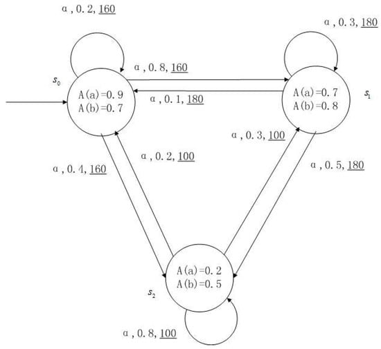
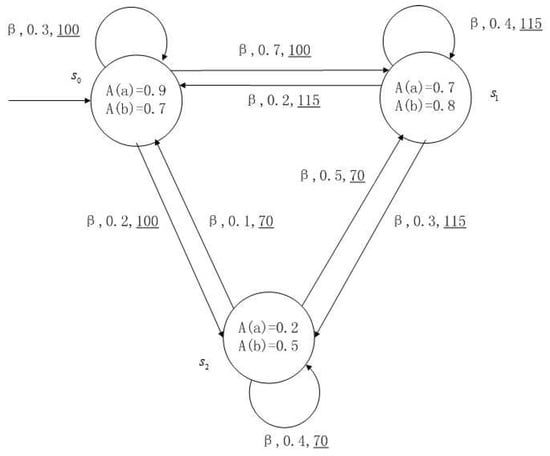
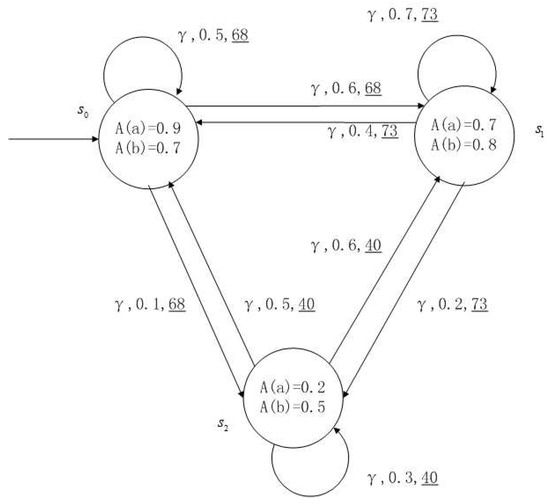
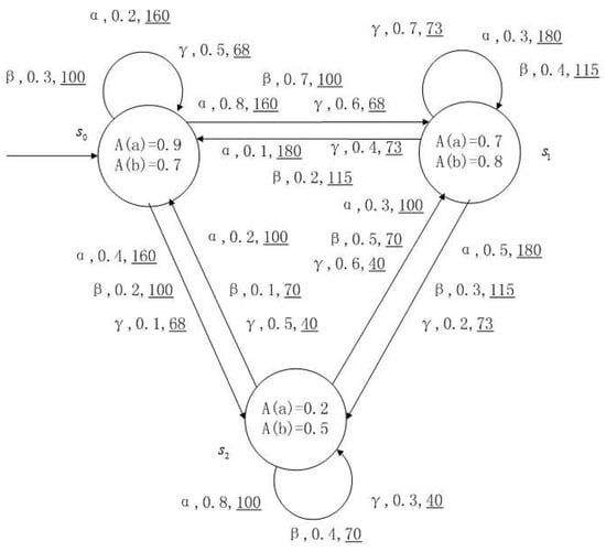
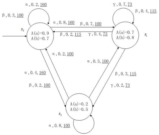
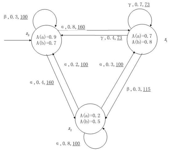
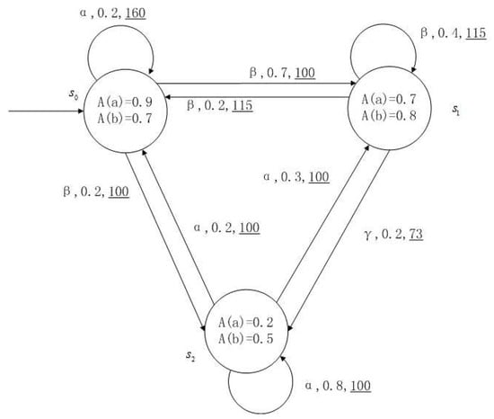
Figure 1, Figure 2, Figure 3 and Figure 4 is a simple, in which there are three transitions represented by α, β and γ. The model has three states , and . The variables in the state indicate the atomic proposition a and b. Different states have different memberships of atomic propositions. Therefore, we use fuzzy values to describe them. When action is used in state , cost function is generated. When using a single transition α or β or γ, the FKSs are shown in Figure 1, Figure 2 and Figure 3. The FDPC produced by them is shown in Figure 4. The transition possibility is given by the number on the connecting line, and the cost is indicated by the underlined number in the figure. For example, indicates that in state , using treatment scheme α, the possibility of transition to state is 0.8, and the treatment cost is 160.
Figure 1.
FKS transmitted by .
Figure 2.
FKS transmitted by .
Figure 3.
FKS transmitted by .
Figure 4.
FDPC created by above FKSs.
FDPCs are more complex than FKSs because of the interleaving of the transitions. For example, for a states sequence , there is only one possibility in an FKS, but it may be multiple possibilities in a FDPC, such as or or the others. We introduce a scheduler to convert FDPC into FKS with cost. In this way, the relevant methods in FKS can be used.
Definition 7.
Let be a finite FDPC. is a function of . For each , there is .
Under the scheduler , denotes the set of infinite paths which start from the state s, denotes the set of finite paths which start from all initial states in . denotes the set of infinite paths which start from all initial states in .
We often care about the maximum (or minimum) possibility. We select the maximum (or minimum) possibility of transition from state s to t by action in as an example to introduce our thought of scheduler. If there are two or more actions in such that for , we can select the action by the algebraic product . Through the operation of a scheduler, an FDPC can be switched to an FKS with cost.
Remark 1.
It is easy to prove that the select operations do not change the maximum or minimum possibility of the , because we can use the actions which are selected by us to replace the actions in the maximum or minimum possibility path.
Example 2.
For the FDPC of Figure 4, suppose the scheduler function is , , . The FDPC of , the maximum possibility transition FDPC of and the minimum possibility transition FDPC of are shown in Figure 5, Figure 6 and Figure 7. In fact, Figure 6 and Figure 7 are FKSs with cost.
Figure 5.
FDPC of .
Figure 6.
The maximum possibility transition FDPC of .
Figure 7.
The minimum possibility transition FDPC of .
The actions are eliminated in the conversion period, so we design an action index matrix to store those actions. The transition matrix in the corresponding FKS and the index matrix for recording actions under a specific scheduler are given below.
Let be a finite FDPC and be a path of .
is a fuzzy matrix of transition possibility under the action . For each ,
The left of the equation is the direct transition which transmit from s to t in FKS which is transmitted by with cost, but the right is the direct transition which transmit from s to t by act in FDPC.
is a fuzzy matrix which denotes the matrix of maximum transition possibility of . For each ,
is a action index matrix which records the actions creating the maximum transition possibility. For each ,
is a fuzzy matrix which denotes the matrix of minimum transition possibility of . For each ,
is a action index matrix which records the actions creating the minimum transition possibility. For each ,
We often pay attention to the maximum and minimum possibility of FDPC, but they are the special where for all . We use the special symbol to denote the index of this .
is a fuzzy matrix which denotes the matrix of maximum transition possibility of FDPC. For each ,
is a action index matrix which records the actions creating the maximum transition possibility. For each ,
is a fuzzy matrix which denotes the matrix of minimum transition possibility of FDPC. For each ,
is a action index matrix which records the actions creating the minimum transition possibility. For each ,
is a matrix declaring the cost activating action from state s, for each ,
Example 3.
For the FDPC of Figure 4.
The action α transition possibility matrix and the cost matrix activating action α is
The action β transition possibility matrix and the cost matrix activating action β is
The action γ transition possibility matrix and the cost matrix activating action γ is
The maximum transition possibility matrix, maximum transition possibility action index matrix, minimum transition possibility matrix and minimum transition possibility action index matrix is
Under the maximum transition possibility matrix and minimum transition possibility matrix, the FDPC of Figure 4 turns into the FKSs with cost in Figure 8 and Figure 9.
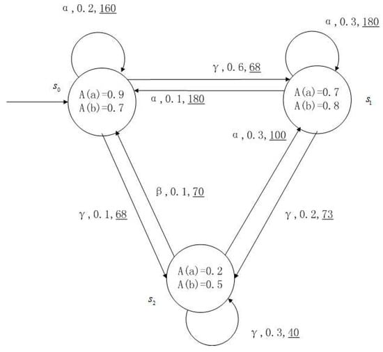
Figure 8.
FDPC of .
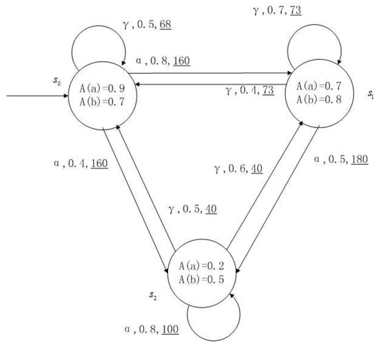
Figure 9.
FDPC of .
Since the cost is generated in the process of each activation action, in order to solve the cost-related problems in model checking, we determine the cost through a deterministic selection strategy for the action, and then calculate the expected cost. Because model checking pays more attention to the possibility of transition, this paper takes the maximum possibility of one-step transition as the selected strategy. First, we select the action by the above matrix. Then, we select the successor state by the maximum possibility.
Definition 8.
Let be a finite FDPC and be a path of . denotes the instantaneous cost of the step k.
Under the scheduler , we use each step to choose the maximum possibility to transmit from the current state as an example, and the step k instantaneous expected cost is defined as
We use to denote the cumulative cost of the first k steps. The cumulative expected cost of the first k steps is defined as
The previous descriptions are all about the expected cost without limiting the states in the path. However, in the actual process, some restrictions may be added to the states in the path.
denotes the cumulative cost that the path would reach the state in F, where , is the prefix of and but the other states in is not in F. denotes the skep n instantaneous expected cost under the scheduler which is the deformation of , defined as below.
denotes the first steps k cumulative expected cost under the scheduler which reaches F in step k, defined as below,
is the cumulative expected cost from s to the state in F, defined as below,
Where n is the max step of all paths that can reach F under the restrictive condition ‘No or one ring’. Why do we have the restrictive condition ‘No or one ring’? Because it has no contribution for transition possibility changing. Without the amount of rings, all states of the path which can reach F are less than or equal , thus we can get that the max skep .
4. FCTL with Cost Operator
We present the FCTL with cost operators in this section, i.e., expand FCTL for our FDPC with cost operator. We expand FCTL [19] with the cost operator. The syntax and semantics are as below.
Definition 9
(FCTL syntax). The FCTL state formula is defined inductively as follows,
where φ is a path formula, .
Furthermore, the FCTL path formula is,
,
where Φ, and are state formulas.
Definition 10
where.
(FCTL semantics). Let be an finite FDPC, be a function. For FCTL with cost, the semantic of state formula Φ is defined as follows.
For the given scheduler and , the semantic of path formula φ is defined as below.
,
5. Model Checking Fuzzy Computation Tree Logic Based on Fuzzy Decision Processes with Cost
The FCTL model checking problem on FDPC is defined as the following. Given a FDPC , a state s of , a FCTL state formula and a step k, then calculate the true value of state s satisfying the state formula or the expect cost. We often consider the maximum and minimum possibilitic truth values. We give the computing method of , , , , , , , , , , , , and as below. There are some useful matrixes and operations given.
Let be a finite FDPC, be a fuzzy diagonal matrix for state formula . For each ,
is a fuzzy matrix. For each ,
We use to realize the transition of only choosing the maximum truth value transition using action . is a fuzzy matrix and defined as that for each ,
where f is a function mapping to [0,1]. f is decided by the need in usual. In this paper, we set if there is only one maximum transition from s to t. When it is multiple, we select the first maximum transition by elements in the matrix.
Through those matrixes, we can reduce the state transition matrix in FKS to a sparse matrix containing only one-step maximum possibility.
E is a fuzzy matrix with all elements equal to 1. We use it to turn the matrix into a vector.
We also use an auxiliary matrix identified as , for the restricted set F. is defined below.
where
is the restricted transition matrix under the act which restrict only transition to F. is the restricted transition matrix under the act which cannot transmit to F. Using matrixes, we can describe the constraints.
Using our matrixes, we can re-represent the cost in Definition 8.
The first k steps cumulative expected cost
The restricted set step k instantaneous expected cost
The restricted set first k steps cumulative expected cost
where is the operation that to first count and second count for . is the operation that to first count and second count for .
is the maximum truth value of that there exists a path that starts from state s and satisfies .
The proof is placed in Appendix A.
is the minimum truth value of that there exists a path that starts from state s and satisfies .
The proof is placed in Appendix A.
is the maximum truth value of that all of the paths which start from state s satisfy .
The proof is placed in Appendix A.
is the minimum truth value of that all of the paths which start from state s satisfy .
The proof is placed in Appendix A.
is the maximum truth value of that there exists a path that starts from state s satisfies .
The proof is placed in Appendix A.
is the minimum truth value of that there exists a path that starts from state s satisfies .
The proof is placed in Appendix A.
is the maximum truth value of that all of the paths which start from state s satisfy .
The proof is placed in Appendix A.
is minimum the truth values of that all of the paths that start from state s satisfy .
The proof is placed in Appendix A.
is the skep k instantaneous expected cost of the path that starts from state s under the maximum scheduler.
where
The proof is placed in Appendix A.
is the skep k instantaneous expected cost of the path that starts from state s under the minimum scheduler.
where
The proof is placed in Appendix A.
is the first k steps cumulative expected cost of the path that starts from state s under the maximum scheduler.
where
is the first k steps cumulative expected cost of the path that starts from state s under the minimum scheduler.
where
is the cumulative expected cost of the path that starts from state s and can reach a state in F under the maximum scheduler.
where ,
if
if
is the cumulative expected cost of the path that starts from state s and can reach a state in F under the minimum scheduler.
where ,
if
if
According to (1)–(14), we provide three algorithms to solve the problem of FCTL model checking with cost. Algorithm 1 is used to catch some values of some parameters which would be used to calculate the cost operators. Algorithm 2 is used to calculate the truth values of the formal FCTL state formulas. Algorithm 3 is used to calculate the cost operators.
| Algorithm 1 Catch the action |
|
Algorithm 1 is proposed to get the action and states and in transition which are used in the computing of cost operators. By the definition of , we can use the to be the determined condition of which is the successor state.
| Algorithm 2 Calculating the formal FCTL state formula |
|
Algorithm 2 is proposed to calculate the quantitative possibility of state formula by matrix operations based on (1)–(8).
Algorithm 3 is proposed to calculate the cost operators by matrix operations based on (9)–(14).
Now let us analyze the time complexities of our algorithm. We would see the three algorithms as one algorithm and analyze it.
Under the scheduler , we can recursively calculate the truth value of in step , which is the number of the sub-formula of which is recursively defined as below. If , then , , , , , , , , and .
The time complexity of calculating the formula is only contacted with the size of FDPC and , and is . The time of calculating the formula is only contacted with the size of FDPC and and k, and is . The time of calculating the formula is mainly contacted with the time of calculating the transitive closure of , e.g., . We use the method of literature [30], and the time complexities is . The time of calculating the formula is contacted with the time of catch and the time of matrix multiplication, and is . Above all, we give the time complexities of our algorithm.
| Algorithm 3 Calculating the cost operators of FCTL |
|
Theorem 1.
Let be a finite FDPC, Φ be a FCTL formula and k be a natural number. Then, the time complexities of calculating the truth values or expected cost is , where is the size of FDPC , is a polynomials of , is the number of the sub-formula of , and k is the given natural number.
6. Illustrative Examples
A medical expert system is an intelligent computer system that collects, sorts and analyzes a large number of cases by computer, concentrates on the diagnosis results of medical experts, and diagnoses and treats patients. Because of the different judgment standards of each expert for the degree of the patient’s conditions and the effect of the treatment plan, using a fuzzy system can reflect the operation process of the system closer to the real world. Figure 10, Figure 11, Figure 12 and Figure 13 is a simple medical expert system, in which there are three experts. Each expert gives different treatment plans, which are represented by , , . The model has four states of the patients, respectively, represented by , , , . The variables in the state indicate the patient’s health states, which can be divided into B(bad), G(general), N(normal) and E(enough). Different experts have a different understanding of these four health conditions. Therefore, we give fuzzy values to the four to show the health of patients. When treatment scheme is used in state , cost will be generated, indicating the treatment cost of the scheme. When using a single treatment scheme, the state transition of patients is shown in Figure 10, Figure 11 and Figure 12. When three experts consult, a complex system is synthesized, as shown in Figure 13. The connecting line with the arrow in the figure indicates transition. The transition possibility is given by the number on the connecting line, and the cost is indicated by the underlined number in the figure. For example, indicates that the patient is in state , using treatment scheme , then the possibility of transition to state is 0.8, and the treatment cost is 160.
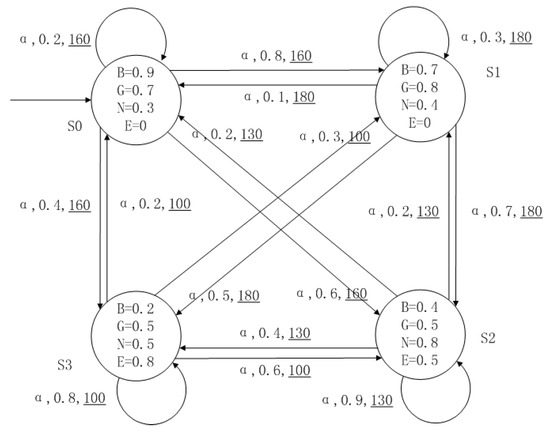
Figure 10.
The model of treatment options .
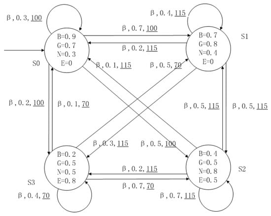
Figure 11.
The model of treatment options .
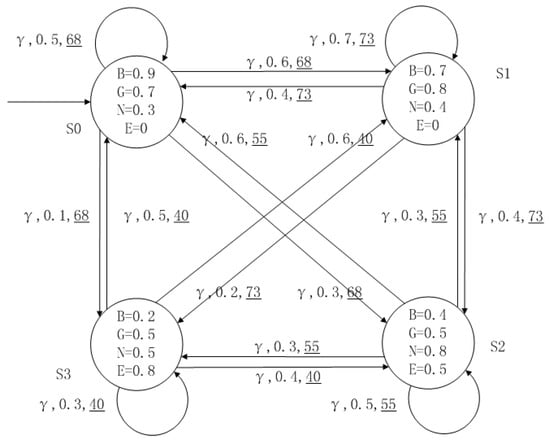
Figure 12.
The model of treatment options .
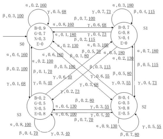
Figure 13.
The FDPC of medical expert system.
(1) , . is the maximum truth value of that there exists one plan where the patient starts from state and becomes normal after one treatment. is the minimum truth value of that there exists one plan where the patient starts from state and becomes normal after one treatment.
(2) , . is the maximum truth value of all of the plans to satisfy that the patient starts from state and becomes general after one treatment. is the minimum truth value of all of the plans to satisfy that the patient starts from state and becomes general after one treatment.
(3) , . is the maximum truth value that there exists one plan that the patient starts from state , keeps general in treatments and becomes enough finally. is the minimum truth value that there exists one plan that the patient starts from state , keeps general in treatments and becomes enough finally.
(4) , . is the maximum truth value that all of the plans to satisfy that the patient starts from state , keeps general in treatments and becomes enough finally. is the minimum truth value that all of the plans to satisfy that the patient starts from state , keeps general in treatments and becomes enough finally.
(5) , . is the maximum skep 6 instantaneous expected cost of that the patient starts from state . is the minimum skep 6 instantaneous expected cost of that the patient starts from state .
(6) , . is the maximum first 6 steps cumulative expected cost of that the patient starts from state . is the minimum first 6 steps cumulative expected cost of that the patient starts from state .
(7) , . is the maximum cumulative expected cost of that the patient starts from state and becomes enough finally. is the minimum cumulative expected cost of that the patient starts from state and becomes enough finally.
7. Conclusions
This paper provides a polynomial model checking algorithm for the verification of some quantitative properties in fuzzy systems in which in any state a nondeterministic choice and cost between fuzzy sets exist. First, we define a fuzzy decision process model with a cost function. This model can describe the cost consumption and other attributes of a fuzzy system. By introducing the definition of the scheduler, we transmit FDPC into a fuzzy Kripke structure. Next, we give the syntax and semantics of fuzzy computation tree logic with a cost operator to describe the properties. Then, using fuzzy matrix and matrix operations, the quantitative calculation of the computation tree logic model checking on the fuzzy decision process model with the cost is introduced, and the corresponding polynomial time algorithm is proposed.
There are several problems that are worth further study. First, it is interesting to consider the linear temporal logic model checking in FDPC. Second, we would like to extend this method used in this paper to multi-objectives model checking. Finally, we will give some case studies on the methods proposed in this paper.
Author Contributions
Conceptualization and Methodology, Z.M. and Z.L.; Formal analysis, W.L., X.L. and Y.G. All authors have read and agreed to the published version of the manuscript.
Funding
The work is partially supported by National Natural Science Foundation of China (Grant No. 61962001), Graduate Innovation Project of North Minzu University (Grant No. YCX22196 and No. YCX22184), Scientific Research Project of Introducing Personnel from North Minzu University (Grant No. 2020KYQD 14), Provincial key R& D of Ningxia Science and Technology Department (Grant No. 2019BEB04032), and Provincial Natural Science Foundation of Ningxia (Grant No. 2021A1017).
Institutional Review Board Statement
Not applicable.
Informed Consent Statement
Not applicable.
Data Availability Statement
Not applicable.
Conflicts of Interest
The authors declare that they have no known competing financial interests or personal relationships that could have appeared to influence the work reported in this paper.
Appendix A. Proof of (1)–(10)
Proof.
(1)
□
Proof.
(2)
□
Proof.
(3)
□
Proof.
(4)
□
Proof.
(5)
□
Proof.
(6)
□
Proof.
(7)
where,
□
Proof.
(8)
□
Proof.
(9)
where □
Proof.
(10)
where □
References
- Baier, C.; Katoen, J.P. Principles of Model Checking; MIT Press: Cambridge, MA, USA, 2008. [Google Scholar]
- Xie, D.; Xiong, W.; Bu, L.; Li, X. Deriving unbounded reachability proof of linear hybrid automata during bounded checking procedure. IEEE Trans. Comput. 2017, 66, 416–430. [Google Scholar] [CrossRef]
- Rawlings, B.C.; Lafortune, S.; Ydstie, B.E. Supervisory control of labeled transition systems subject to multiple reachability requirements via symbolic model checking. IEEE Trans. Control. Syst. Technol. 2020, 28, 644–652. [Google Scholar] [CrossRef]
- Hart, S.; Sharir, M. Probabilistic propositional temporal logics. Inf. Control. 1986, 70, 97–155. [Google Scholar] [CrossRef]
- Alfaro, L.D.; Kwiatkowska, M.; Norman, G.; Parker, D.; Segala, R. Symbolic model checking of probabilistic processes using mtbdds and the kronecker representation. In Tools and Algorithms for the Construction and Analysis of Systems; Graf, S., Schwartzbach, M., Eds.; Springer: Berlin/Heidelberg, Germany, 2000; pp. 395–410. [Google Scholar]
- Baier, C.; Clarke, E.M.; Hartonas-Garmhausen, V.; Kwiatkowska, M.; Ryan, M. Symbolic model checking for probabilistic processes. In International Colloquium on Automata, Languages, and Programming; Degano, P., Gorrieri, R., Marchetti-Spaccamela, A., Eds.; Springer: Berlin/Heidelberg, Germany, 1997; pp. 430–440. [Google Scholar] [CrossRef]
- Baier, C.; Ciesinski, F.; Grosser, M. Probmela: A Modeling Language for Communicating Probabilistic Processes. In Proceedings of the Second ACM and IEEE International Conference on Formal Methods and Models for Co-Design, San Diego, CA, USA, 23–25 June 2004; Volume 4, pp. 57–66. [Google Scholar]
- Baier, C.; de Alfaro, L.; Forejt, V.; Kwiatkowska, M. Model Checking Probabilistic Systems; Springer International Publishing: Cham, Switzerland, 2018; pp. 963–999. [Google Scholar] [CrossRef]
- Chechik, M.; Gurfinkel, A.; Devereux, B. Xchek: A Multi-Valued Model-Checker. In Computer Aided Verification; Brinksma, E., Larsen, K.G., Eds.; Springer: Berlin/Heidelberg, Germany, 2002; pp. 505–509. [Google Scholar] [CrossRef]
- Chechik, M.; Easterbrook, S.; Devereux, B. Model checking with multi-valued temporal logics. In Proceedings of the 31st IEEE International Symposium on Multiple-Valued Logic, Warsaw, Poland, 22–24 May 2001; IEEE: Warsaw, Poland, 2001; pp. 187–192. [Google Scholar]
- Li, Y.; Droste, M.; Lei, L. Model checking of linear-time properties in multi-valued systems. Inf. Sci. 2017, 377, 51–74. [Google Scholar] [CrossRef]
- Chechik, M.; Gurfinkel, A.; Devereux, B.; Lai, A.; Easterbrook, S. Data structures for symbolic multi-valued model-checking. Form. Methods Syst. Des. 2006, 29, 295–344. [Google Scholar] [CrossRef]
- Li, Y.; Li, L. Model checking of linear-time properties based on possibility measure. IEEE Trans. Fuzzy Syst. 2013, 21, 842–854. [Google Scholar] [CrossRef]
- Li, Y.; Li, Y.; Ma, Z. Computation tree logic model checking based on possibility measures. Fuzzy Sets Syst. 2015, 262, 44–59. [Google Scholar] [CrossRef] [Green Version]
- Li, Y.; Ma, Z. Quantitative computation tree logic model checking based on generalized possibility measures. IEEE Trans. Fuzzy Syst. 2015, 23, 2034–2047. [Google Scholar] [CrossRef]
- Zhang, S.; Li, Y. Expressive power of linear-temporal logic based on generalized possibility measures. In Proceedings of the 2016 IEEE International Conference on Fuzzy Systems (FUZZ-IEEE), Vancouver, BC, Canada, 24–29 July 2016; pp. 431–436. [Google Scholar]
- Subhankar Mukherjee, P.D. A fuzzy real-time temporal logic. Int. J. Approx. Reason. 2013, 54, 1452–1470. [Google Scholar] [CrossRef]
- Yang, C.; Li, Y. ϵ-bisimulation relations for fuzzy automata. IEEE Trans. Fuzzy Syst. 2018, 26, 2017–2029. [Google Scholar] [CrossRef]
- Pan, H.; Li, Y.; Cao, Y.; Ma, Z. Model checking fuzzy computation tree logic. Fuzzy Sets Syst. 2015, 262, 60–77. [Google Scholar] [CrossRef]
- Zadeh, L. Fuzzy sets. Inf. Cont. 1965, 8, 338–353. [Google Scholar] [CrossRef]
- Zimmermann, H.-J. Fuzzy Set Theory and Its Applications; Springer: Dordrecht, The Netherlands, 2001. [Google Scholar]
- Frigeri, A.; Pasquale, L.; Spoletini, P. Fuzzy time in linear temporal logic. ACM Trans. Comput. Log. 2014, 15, 1–22. [Google Scholar] [CrossRef]
- Garmendia Salvador, L.; González del Campo, R.; López, V.; Recasens Ferrés, J. An algorithm to compute the transitive closure, a transitive approximation and a transitive opening of a proximity. Mathw. Soft Comput. 2009, 16, 175–191. [Google Scholar]
- Zhang, P.; Jiang, J.; Ma, Z.; Zhu, H. Quantitative μ-calculus model checking algorithm based on generalized possibility measures. In Proceedings of the 2019 IEEE Intl Conference on Dependable, Autonomic and Secure Computing, International Conference on Pervasive Intelligence and Computing, International Conference on Cloud and Big Data Computing, International Conference on Cyber Science and Technology Congress (DASC/PiCom/CBDCom/CyberSciTech), Fukuoka, Japan, 5–8 August 2019; IEEE: Piscataway, NJ, USA, 2019; pp. 449–453. [Google Scholar] [CrossRef]
- Choi, J.; Lee, K.Y. Fuzzy Decision Making for TEP; Wiley-IEEE Press: Piscataway, NJ, USA, 2022; pp. 375–399. [Google Scholar]
- Li, Y.; Wei, J. Possibilistic fuzzy linear temporal logic and its model checking. IEEE Trans. Fuzzy Syst. 2021, 29, 1899–1913. [Google Scholar] [CrossRef]
- Yang, W.; Jhang, S.; Shi, S.E.A. A novel additive consistency for intuitionistic fuzzy preference relations in group decision making. Appl. Intell. 2020, 50, 4342–4356. [Google Scholar] [CrossRef]
- Xue, Y.; Deng, Y. Decision making under measure-based granular uncertainty with intuitionistic fuzzy sets. Appl. Intell. 2021, 51, 6224–6233. [Google Scholar] [CrossRef] [PubMed]
- Li, Y.M. Analysis of Fuzzy Systems; Science Press: Beijing, China, 2005. (In Chinese) [Google Scholar]
- Zhang, Y.; Tang, J.; Meng, F. Programming model-based method for ranking objects from group decision making with interval-valued hesitant fuzzy preference relations. Appl. Intell. 2019, 49, 837–857. [Google Scholar] [CrossRef]
Publisher’s Note: MDPI stays neutral with regard to jurisdictional claims in published maps and institutional affiliations. |
© 2022 by the authors. Licensee MDPI, Basel, Switzerland. This article is an open access article distributed under the terms and conditions of the Creative Commons Attribution (CC BY) license (https://creativecommons.org/licenses/by/4.0/).