
A Survey on Applications of H-Technique: Revisiting Security Analysis of PRP and PRF


Abstract
:1. Introduction
1.1. Revisiting Some Popular Proof Techniques
1.2. Our Contribution
Organization of the Paper
2. Preliminaries
2.1. Notation
- A pair of tuples is referred to as function-compatible if . We denote it as .
- A pair of tuples is referred to as permutation-compatible if . We denote it as .
- A pair of triples is referred to as tweakable-permutation-compatible if . We denote it as (equivalently, ).
2.2. Statistical Distance
- 1.
- (non-negative) .
- 2.
- (identification) if and only if .
- 3.
- (symmetric) .
- 4.
- Triangle inequality(general form):
- 5.
- . The equality holds if and only if the supports of these two probability functions are disjoint.
3. Models for Interactive Algorithms
3.1. Probabilistic Function
3.2. Function Models of Interactive Algorithms and Their Interaction
- Joint Response Function:- A q-joint response function is a probabilistic function such that for all random coins r, the mapping is functionally independent of .
- Joint Query Function:- A probabilistic function is called aq-joint query function if for all random coins r, the mapping isfunctionally independent of . Moreover, it is called
- -
- nonadaptive if is functionally independent of and
- -
- deterministic if the random coin space is a singleton (we simply drop the random coin space notation and write it as a function ).
3.3. Examples of Response Functions
Some Ideal Random Systems
4. H-Technique Tools
4.1. Distinguisher and Its Advantage
- The algorithm obtains a transcript .
- The function b finally makes a decision based on the transcript and the random coin initially sampled by .
| . |
Conventions
- Distinguishers are deterministic: Given any query function , and for a fixed random coin r, let denote the deterministic query function which basically runs with the random coin r. It is easy to verify that and hence there exists for which . Hence,
- No redundant queries: In this paper we only consider deterministic keyed functions. An adversary interacting with a deterministic keyed function is called redundant if makes two identical queries (i.e., for some ). An adversary interacting with a deterministic keyed strong permutation is called redundant if for some , or , where is the response of the ith query. Note that, in this case, , where denotes the forward-only transcript. The response of jth query is uniquely determined from the ith query. Similarly, we define redundant queries for a tweakable keyed permutation. The ith query is called redundant if there is with , either or .
4.2. Security Definitions
- ,
- ,
- ,
- ,
- ,
- ,
- .
4.3. H-Technique
4.4. Expectation Method
5. Hash-Based Constructions
5.1. Hash-Then-PRF
- there exist distinct , such that .
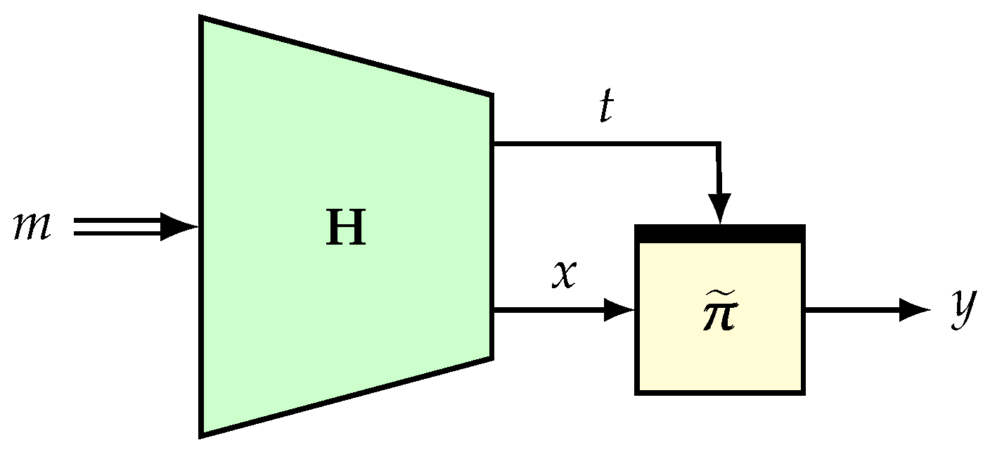
5.2. Hash-Then-TBC
5.2.1. A. Proof without Releasing the Internal Values
- no collision among and
- no collision among .
(1) Standard H-Technique:
(2) Expectation Method:
5.2.2. B. Proof by Releasing the Internal Values
- there is a collision among or
- there is a collision among .
5.3. An Extension of Naor–Reingold
- –
- Input: .
- .
- , where and .
- .
- .
- return .
5.3.1. A Simple Proof for ENR
5.3.2. A Simple Proof for LDT
6. Feistel Structure-Based Schemes
6.1. Three-Round Luby–Rackoff
6.2. Three-Round TBC-Based Luby–Rackoff
- for all ,
- for all ,
7. Strong Pseudo-Random Permutation Designs
7.1. HCTR
- –
- Input: , ;Output: .
- .
- .
- .
- .
- .
- , such that .
- , such that .
- , such that .
- or for some , , ,
- or , , .
7.2. TET
8. Beyond-Birthday-Bound Secure Schemes
8.1. Pseudorandom Functions
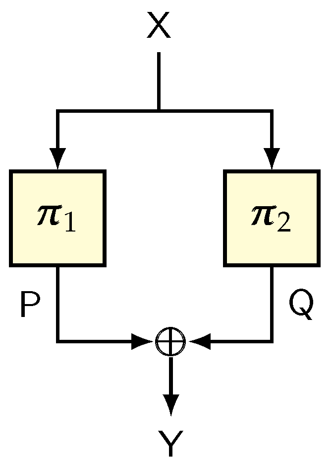
8.1.1. Sum of Permutations
8.1.2. Sum of Even-Mansour
- : and .
- : and .
- : and .
9. Optimality of the Extended H-Technique
Nonadaptive PRP to SPRP
10. Conclusions
Author Contributions
Funding
Conflicts of Interest
References
- Goldreich, O.; Goldwasser, S.; Micali, S. How to Construct Random Functions (Extended Abstract). In Proceedings of the 25th Annual Symposium on Foundations of Computer Science, West Palm Beach, FL, USA, 24–26 October 1984; pp. 464–479. [Google Scholar]
- Luby, M.; Rackoff, C. How to Construct Pseudo-Random Permutations from Pseudo-Random Functions (Abstract). In Proceedings of the Advances in Cryptology—CRYPTO ’85, Santa Barbara, CA, USA, 18–22 August 1985; p. 447. [Google Scholar]
- Bellare, M.; Rogaway, P. The Security of Triple Encryption and a Framework for Code-Based Game-Playing Proofs. In Proceedings of the Advances in Cryptology—EUROCRYPT 2006, 25th Annual International Conference on the Theory and Applications of Cryptographic Techniques, St. Petersburg, Russia, 28 May–1 June 2006; pp. 409–426. [Google Scholar]
- Shoup, V. Sequences of games: A tool for taming complexity in security proofs. IACR Cryptol. Eprint Arch. 2004, 2004, 332. [Google Scholar]
- Goldwasser, S.; Micali, S. Probabilistic Encryption. J. Comput. Syst. Sci. 1984, 28, 270–299. [Google Scholar] [CrossRef] [Green Version]
- Yao, A.C. Theory and Applications of Trapdoor Functions (Extended Abstract). In Proceedings of the 23rd Annual Symposium on Foundations of Computer Science, Chicago, IL, USA, 3–5 November 1982; pp. 80–91. [Google Scholar]
- Shoup, V. Using Hash Functions as a Hedge against Chosen Ciphertext Attack. In Proceedings of the Advances in Cryptology—EUROCRYPT 2000, International Conference on the Theory and Application of Cryptographic Techniques, Bruges, Belgium, 14–18 May 2000; pp. 275–288. [Google Scholar]
- Shoup, V. OAEP Reconsidered. J. Cryptol. 2002, 15, 223–249. [Google Scholar] [CrossRef]
- Cramer, R.; Shoup, V. Design and Analysis of Practical Public-Key Encryption Schemes Secure against Adaptive Chosen Ciphertext Attack. SIAM J. Comput. 2003, 33, 167–226. [Google Scholar] [CrossRef]
- Camenisch, J.; Shoup, V. Practical Verifiable Encryption and Decryption of Discrete Logarithms. In Proceedings of the Advances in Cryptology—CRYPTO 2003, 23rd Annual International Cryptology Conference, Santa Barbara, CA, USA, 17–21 August 2003; pp. 126–144. [Google Scholar]
- Abe, M.; Gennaro, R.; Kurosawa, K.; Shoup, V. Tag-KEM/DEM: A New Framework for Hybrid Encryption and A New Analysis of Kurosawa-Desmedt KEM. In Proceedings of the Advances in Cryptology—EUROCRYPT 2005, 24th Annual International Conference on the Theory and Applications of Cryptographic Techniques, Aarhus, Denmark, 22–26 May 2005; pp. 128–146. [Google Scholar]
- Landecker, W.; Shrimpton, T.; Terashima, R.S. Tweakable Blockciphers with Beyond Birthday-Bound Security. In Proceedings of the Advances in Cryptology—CRYPTO 2012—32nd Annual Cryptology Conference, Santa Barbara, CA, USA, 19–23 August 2012; pp. 14–30. [Google Scholar]
- Bellare, M.; Kilian, J.; Rogaway, P. The Security of the Cipher Block Chaining Message Authentication Code. J. Comput. Syst. Sci. 2000, 61, 362–399. [Google Scholar] [CrossRef] [Green Version]
- Bellare, M.; Pietrzak, K.; Rogaway, P. Improved Security Analyses for CBC MACs. In Advances in Cryptology—CRYPTO 2005; Springer: Berlin/Heidelberg, Germany, 2005; pp. 527–545. [Google Scholar]
- Black, J.; Rogaway, P. CBC MACs for Arbitrary-Length Messages: The Three-Key Constructions. J. Cryptol. 2005, 18, 111–131. [Google Scholar] [CrossRef] [Green Version]
- Yasuda, K. The Sum of CBC MACs Is a Secure PRF. In Proceedings of the Topics in Cryptology—CT-RSA 2010, The Cryptographers’ Track at the RSA Conference 2010, San Francisco, CA, USA, 1–5 March 2010; pp. 366–381. [Google Scholar]
- Yasuda, K. A New Variant of PMAC: Beyond the Birthday Bound. In Proceedings of the Advances in Cryptology—CRYPTO 2011—31st Annual Cryptology Conference, Santa Barbara, CA, USA, 14–18 August 2011; pp. 596–609. [Google Scholar]
- Halevi, S.; Rogaway, P. A Tweakable Enciphering Mode. In Proceedings of the Advances in Cryptology—CRYPTO 2003, 23rd Annual International Cryptology Conference, Santa Barbara, CA, USA, 17–21 August 2003; pp. 482–499. [Google Scholar]
- Halevi, S.; Rogaway, P. A Parallelizable Enciphering Mode. In Proceedings of the Topics in Cryptology—CT-RSA 2004, The Cryptographers’ Track at the RSA Conference 2004, San Francisco, CA, USA, 23–27 February 2004; pp. 292–304. [Google Scholar]
- Halevi, S. Invertible Universal Hashing and the TET Encryption Mode. In Proceedings of the Advances in Cryptology—CRYPTO 2007, 27th Annual International Cryptology Conference, Santa Barbara, CA, USA, 19–23 August 2007; pp. 412–429. [Google Scholar]
- Chakraborty, D.; Sarkar, P. HCH: A New Tweakable Enciphering Scheme Using the Hash-Counter-Hash Approach. IEEE Trans. Inf. Theory 2008, 54, 1683–1699. [Google Scholar] [CrossRef]
- Wang, P.; Feng, D.; Wu, W. HCTR: A Variable-Input-Length Enciphering Mode. In Proceedings of the Information Security and Cryptology: First SKLOIS Conference, CISC 2005, Beijing, China, 15–17 December 2005; pp. 175–188. [Google Scholar]
- Ristenpart, T.; Rogaway, P. How to Enrich the Message Space of a Cipher. In Proceedings of the Fast Software Encryption, 14th International Workshop, FSE 2007, Luxembourg, 26–28 March 2007; Revised Selected Papers. pp. 101–118. [Google Scholar]
- Sarkar, P. Improving Upon the TET Mode of Operation. In Proceedings of the Information Security and Cryptology—ICISC 2007, 10th International Conference, Seoul, Korea, 29–30 November 2007; pp. 180–192. [Google Scholar]
- Sarkar, P. Efficient tweakable enciphering schemes from (block-wise) universal hash functions. IEEE Trans. Inf. Theory 2009, 55, 4749–4760. [Google Scholar] [CrossRef] [Green Version]
- Bellare, M.; Boldyreva, A.; Knudsen, L.R.; Namprempre, C. On-line Ciphers and the Hash-CBC Constructions. J. Cryptol. 2012, 25, 640–679. [Google Scholar] [CrossRef]
- Rogaway, P.; Zhang, H. Online Ciphers from Tweakable Blockciphers. In Proceedings of the Topics in Cryptology—CT-RSA 2011—The Cryptographers’ Track at the RSA Conference 2011, San Francisco, CA, USA, 14–18 February 2011; pp. 237–249. [Google Scholar]
- Forler, C.; List, E.; Lucks, S.; Wenzel, J. POEx: A Beyond-Birthday-Bound-Secure On-Line Cipher. In Proceedings of the ArcticCrypt 2016, Svalbard, Norway, 17–22 July 2016; Available online: https://www.researchgate.net/publication/299565944_POEx_A_Beyond-Birthday-Bound-Secure_On-Line_Cipher (accessed on 3 January 2022).
- Jha, A.; Nandi, M. On rate-1 and beyond-the-birthday bound secure online ciphers using tweakable block ciphers. Cryptogr. Commun. 2018, 10, 731–753. [Google Scholar] [CrossRef]
- Rogaway, P.; Shrimpton, T. A Provable-Security Treatment of the Key-Wrap Problem. In Proceedings of the Advances in Cryptology—EUROCRYPT 2006, 25th Annual International Conference on the Theory and Applications of Cryptographic Techniques, St. Petersburg, Russia, 28 May–1 June 2006; pp. 373–390. [Google Scholar]
- Rogaway, P.; Bellare, M.; Black, J.; Krovetz, T. OCB: A block-cipher mode of operation for efficient authenticated encryption. In Proceedings of the CCS 2001, Philadelphia, PA, USA, 6–8 November 2001; pp. 196–205. [Google Scholar]
- Rogaway, P. Efficient Instantiations of Tweakable Blockciphers and Refinements to Modes OCB and PMAC. In Proceedings of the Advances in Cryptology—ASIACRYPT 2004, 10th International Conference on the Theory and Application of Cryptology and Information Security, Jeju Island, Korea, 5–9 December 2004; pp. 16–31. [Google Scholar]
- Krovetz, T.; Rogaway, P. The Software Performance of Authenticated-Encryption Modes. In Proceedings of the Fast Software Encryption—18th International Workshop (FSE 2011), Lyngby, Denmark, 13–16 February 2011; Revised Selected Papers. pp. 306–327. [Google Scholar]
- Andreeva, E.; Bogdanov, A.; Luykx, A.; Mennink, B.; Tischhauser, E.; Yasuda, K. Parallelizable and Authenticated Online Ciphers. In Proceedings of the Advances in Cryptology—ASIACRYPT 2013—19th International Conference on the Theory and Application of Cryptology and Information Security, Bengaluru, India, 1–5 December 2013; Part I. pp. 424–443. [Google Scholar]
- Abed, F.; Fluhrer, S.R.; Forler, C.; List, E.; Lucks, S.; McGrew, D.A.; Wenzel, J. Pipelineable On-line Encryption. In Proceedings of the Fast Software Encryption—21st International Workshop, FSE 2014, London, UK, 3–5 March 2014; Revised Selected Papers. pp. 205–223. [Google Scholar]
- Patarin, J. The “Coefficients H” Technique. In Proceedings of the Selected Areas in Cryptography, 15th International Workshop, SAC 2008, Sackville, NB, Canada, 14–15 August 2008; Revised Selected Papers. pp. 328–345. [Google Scholar]
- Patarin, J. Pseudorandom permutations based on the DES scheme. In Proceedings of the EUROCODE ’90, International Symposium on Coding Theory and Applications, Udine, Italy, 5–9 November 1990; pp. 193–204. [Google Scholar]
- Patarin, J. Etude des Générateurs de Permutations Pseudo-Aléatoires Basés sur le Schéma du DES. Ph.D. Thesis, Université de Paris, Paris, France, 1991. [Google Scholar]
- Patarin, J. Improved Security Bounds for Pseudorandom Permutations. In Proceedings of the 4th ACM Conference on Computer and Communications Security (CCS ’97), Zurich, Switzerland, 1–4 April 1997; pp. 142–150. [Google Scholar]
- Patarin, J. About Feistel Schemes with Six (or More) Rounds. In Proceedings of the Fast Software Encryption, 5th International Workshop (FSE ’98), Paris, France, 23–25 March 1998; pp. 103–121. [Google Scholar]
- Patarin, J. Luby-Rackoff: 7 Rounds Are Enough for 2n(1-epsilon)Security. In Proceedings of the Advances in Cryptology—CRYPTO 2003, 23rd Annual International Cryptology Conference, Santa Barbara, CA, USA, 17–21 August 2003; pp. 513–529. [Google Scholar]
- Vaudenay, S. Decorrelation: A Theory for Block Cipher Security. J. Cryptol. 2003, 16, 249–286. [Google Scholar] [CrossRef] [Green Version]
- Bernstein, D.J. How to Stretch Random Functions: The Security of Protected Counter Sums. J. Cryptol. 1999, 12, 185–192. [Google Scholar] [CrossRef]
- Nandi, M. A Simple and Unified Method of Proving Indistinguishability. In Proceedings of the Progress in Cryptology—INDOCRYPT 2006, 7th International Conference on Cryptology in India, Kolkata, India, 11–13 December 2006; pp. 317–334. [Google Scholar]
- Chen, S.; Steinberger, J.P. Tight Security Bounds for Key-Alternating Ciphers. In Proceedings of the Advances in Cryptology—EUROCRYPT 2014—33rd Annual International Conference on the Theory and Applications of Cryptographic Techniques, Copenhagen, Denmark, 11–15 May 2014; pp. 327–350. [Google Scholar]
- Mouha, N.; Mennink, B.; Herrewege, A.V.; Watanabe, D.; Preneel, B.; Verbauwhede, I. Chaskey: An Efficient MAC Algorithm for 32-bit Microcontrollers. In Proceedings of the Selected Areas in Cryptography—SAC 2014—21st International Conference, Montreal, QC, Canada, 14–15 August 2014; Revised Selected Papers. pp. 306–323. [Google Scholar]
- Mennink, B. Optimally Secure Tweakable Blockciphers. In Proceedings of the Fast Software Encryption—22nd International Workshop (FSE 2015), Istanbul, Turkey, 8–11 March 2015; Revised Selected Papers. pp. 428–448. [Google Scholar]
- Patarin, J. Security of Random Feistel Schemes with 5 or More Rounds. In Proceedings of the Advances in Cryptology—CRYPTO 2004, 24th Annual International CryptologyConference, Santa Barbara, CA, USA, 15–19 August 2004; pp. 106–122. [Google Scholar]
- Nandi, M. The Characterization of Luby-Rackoff and Its Optimum Single-Key Variants. In Proceedings of the Progress in Cryptology—INDOCRYPT 2010—11th International Conference on Cryptology in India, Hyderabad, India, 12–15 December 2010; pp. 82–97. [Google Scholar]
- Nandi, M. Two New Efficient CCA-Secure Online Ciphers: MHCBC and MCBC. In Proceedings of the Progress in Cryptology—INDOCRYPT 2008, 9th International Conference on Cryptology in India, Kharagpur, India, 14–17 December 2008; pp. 350–362. [Google Scholar]
- Lampe, R.; Patarin, J.; Seurin, Y. An Asymptotically Tight Security Analysis of the Iterated Even-Mansour Cipher. In Proceedings of the Advances in Cryptology—ASIACRYPT 2012, 18th International Conference on the Theory and Application of Cryptology and Information Security, Beijing, China, 2–6 December 2012; pp. 278–295. [Google Scholar]
- Chen, S.; Lampe, R.; Lee, J.; Seurin, Y.; Steinberger, J.P. Minimizing the Two-Round Even-Mansour Cipher. In Proceedings of the Advances in Cryptology—CRYPTO 2014, 34th Annual Cryptology Conference, Santa Barbara, CA, USA, 17–21 August 2014; Part I. pp. 39–56. [Google Scholar]
- Cogliati, B.; Seurin, Y. On the Provable Security of the Iterated Even-Mansour Cipher Against Related-Key and Chosen-Key Attacks. In Proceedings of the Advances in Cryptology—EUROCRYPT 2015, 34th Annual International Conference on the Theory and Applications of Cryptographic Techniques, Sofia, Bulgaria, 26–30 April 2015; Part I. pp. 584–613. [Google Scholar]
- Cogliati, B.; Lampe, R.; Seurin, Y. Tweaking Even-Mansour Ciphers. In Proceedings of the Advances in Cryptology—CRYPTO 2015, 35th Annual Cryptology Conference, Santa Barbara, CA, USA, 16–20 August 2015; Part I. pp. 189–208. [Google Scholar]
- Cogliati, B.; Seurin, Y. Beyond-Birthday-Bound Security for Tweakable Even-Mansour Ciphers with Linear Tweak and Key Mixing. In Proceedings of the Advances in Cryptology—ASIACRYPT 2015—21st International Conference on the Theory and Application of Cryptology and Information Security, Auckland, New Zealand, 29 November–3 December 2015; Part II. pp. 134–158. [Google Scholar]
- Bhaumik, R.; Nandi, M. An Inverse-Free Single-Keyed Tweakable Enciphering Scheme. In Proceedings of the Advances in Cryptology—ASIACRYPT 2015—21st International Conference on the Theory and Application of Cryptology and Information Security, Auckland, New Zealand, 29 November–3 December 2015; Part II. pp. 159–180. [Google Scholar]
- Bhaumik, R.; Nandi, M. OleF: An Inverse-Free Online Cipher. An Online SPRP with an Optimal Inverse-Free Construction. IACR Trans. Symmetric Cryptol. 2016, 2016, 30–51. [Google Scholar] [CrossRef]
- Chen, Y.L.; Luykx, A.; Mennink, B.; Preneel, B. Efficient Length Doubling From Tweakable Block Ciphers. IACR Trans. Symmetric Cryptol. 2017, 2017, 253–270. [Google Scholar] [CrossRef]
- Mennink, B. Towards Tight Security of Cascaded LRW2. In Proceedings of the Theory of Cryptography—16th International Conference, TCC 2018, Panaji, India, 11–14 November 2018; Part II. pp. 192–222. [Google Scholar]
- Jha, A.; Nandi, M. Revisiting Structure Graphs: Applications to CBC-MAC and EMAC. J. Math. Cryptol. 2016, 10, 157–180. [Google Scholar] [CrossRef]
- Cogliati, B.; Seurin, Y. EWCDM: An Efficient, Beyond-Birthday Secure, Nonce-Misuse Resistant MAC. In Proceedings of the Advances in Cryptology—CRYPTO 2016—36th Annual International Cryptology Conference, Santa Barbara, CA, USA, 14–18 August 2016; Part I. pp. 121–149. [Google Scholar]
- Mennink, B.; Neves, S. Encrypted Davies-Meyer and Its Dual: Towards Optimal Security Using Mirror Theory. In Proceedings of the Advances in Cryptology—CRYPTO 2017—37th Annual International Cryptology Conference, Santa Barbara, CA, USA, 20–24 August 2017; Part III. pp. 556–583. [Google Scholar]
- Cogliati, B.; Lee, J.; Seurin, Y. New Constructions of MACs from (Tweakable) Block Ciphers. IACR Trans. Symmetric Cryptol. 2017, 2017, 27–58. [Google Scholar] [CrossRef]
- Datta, N.; Dutta, A.; Nandi, M.; Paul, G.; Zhang, L. Single Key Variant of PMAC_Plus. IACR Trans. Symmetric Cryptol. 2017, 2017, 268–305. [Google Scholar] [CrossRef]
- Dutta, A.; Jha, A.; Nandi, M. Tight Security Analysis of EHtM MAC. IACR Trans. Symmetric Cryptol. 2017, 2017, 130–150. [Google Scholar] [CrossRef]
- List, E.; Nandi, M. ZMAC+—An Efficient Variable-output-length Variant of ZMAC. IACR Trans. Symmetric Cryptol. 2017, 2017, 306–325. [Google Scholar] [CrossRef]
- Datta, N.; Dutta, A.; Nandi, M.; Yasuda, K. Encrypt or Decrypt? To Make a Single-Key Beyond Birthday Secure Nonce-Based MAC. IACR Cryptol. Eprint Arch. 2018, 2018, 500. [Google Scholar]
- Datta, N.; Nandi, M. ELmE: A Misuse Resistant Parallel Authenticated Encryption. In Proceedings of the Information Security and Privacy—19th Australasian Conference, ACISP 2014, Wollongong, Australia, 7–9 July 2014; pp. 306–321. [Google Scholar]
- Chakraborti, A.; Iwata, T.; Minematsu, K.; Nandi, M. Blockcipher-Based Authenticated Encryption: How Small Can We Go? In Proceedings of the Cryptographic Hardware and Embedded Systems—CHES 2017—19th International Conference, Taipei, Taiwan, 25–28 September 2017; pp. 277–298. [Google Scholar]
- Bhaumik, R.; Nandi, M. Improved Security for OCB3. In Proceedings of the Advances in Cryptology—ASIACRYPT 2017—23rd International Conference on the Theory and Applications of Cryptology and Information Security, Hong Kong, China, 3–7 December 2017; Part II. pp. 638–666. [Google Scholar]
- Chakraborti, A.; Datta, N.; Nandi, M.; Yasuda, K. Beetle Family of Lightweight and Secure Authenticated Encryption Ciphers. IACR Trans. Cryptogr. Hardw. Embed. Syst. 2018, 2018, 218–241. [Google Scholar] [CrossRef]
- Bose, P.; Hoang, V.T.; Tessaro, S. Revisiting AES-GCM-SIV: Multi-user Security, Faster Key Derivation, and Better Bounds. In Proceedings of the Advances in Cryptology—EUROCRYPT 2018—37th Annual International Conference on the Theory and Applications of Cryptographic Techniques, Tel Aviv, Israel, 29 April–3 May 2018; Part I. pp. 468–499. [Google Scholar]
- Maurer, U.M. Indistinguishability of Random Systems. In Proceedings of the Advances in Cryptology—EUROCRYPT 2002, International Conference on the Theory and Applications of Cryptographic Techniques, Amsterdam, The Netherlands, 28 April–2 May 2002; pp. 110–132. [Google Scholar]
- Maurer, U.M.; Pietrzak, K. The Security of Many-Round Luby-Rackoff Pseudo-Random Permutations. In Proceedings of the Advances in Cryptology—EUROCRYPT 2003, International Conference on the Theory and Applications of Cryptographic Techniques, Warsaw, Poland, 4–8 May 2003; pp. 544–561. [Google Scholar]
- Maurer, U.M.; Pietrzak, K. Composition of Random Systems: When Two Weak Make One Strong. In Proceedings of the Theory of Cryptography, First Theory of Cryptography Conference (TCC 2004), Cambridge, MA, USA, 19–21 February 2004; pp. 410–427. [Google Scholar]
- Maurer, U.M.; Pietrzak, K.; Renner, R. Indistinguishability Amplification. In Proceedings of the Advances in Cryptology—CRYPTO 2007, 27th Annual International Cryptology Conference, Santa Barbara, CA, USA, 19–23 August 2007; pp. 130–149. [Google Scholar]
- Minematsu, K.; Matsushima, T. New Bounds for PMAC, TMAC, and XCBC. In Proceedings of the Fast Software Encryption (FSE 2007), Luxembourg, 26–28 March 2007; pp. 434–451. [Google Scholar]
- Minematsu, K. Beyond-Birthday-Bound Security Based on Tweakable Block Cipher. In Proceedings of the Fast Software Encryption, 16th International Workshop (FSE 2009), Leuven, Belgium, 22–25 February 2009; Revised Selected Papers. pp. 308–326. [Google Scholar]
- Minematsu, K.; Iwata, T. Building Blockcipher from Tweakable Blockcipher: Extending FSE 2009 Proposal. In Proceedings of the Cryptography and Coding—13th IMA International Conference (IMACC 2011), Oxford, UK, 12–15 December 2011; pp. 391–412. [Google Scholar]
- Minematsu, K. Building blockcipher from small-block tweakable blockcipher. Des. Codes Cryptogr. 2015, 74, 645–663. [Google Scholar] [CrossRef]
- Minematsu, K.; Iwata, T. Tweak-Length Extension for Tweakable Blockciphers. In Proceedings of the Cryptography and Coding—15th IMA International Conference (IMACC 2015), Oxford, UK, 15–17 December 2015; pp. 77–93. [Google Scholar]
- Hoang, V.T.; Tessaro, S. Key-Alternating Ciphers and Key-Length Extension: Exact Bounds and Multi-user Security. In Proceedings of the Advances in Cryptology—CRYPTO 2016—36th Annual International Cryptology Conference, Santa Barbara, CA, USA, 14–18 August 2016; Part I. pp. 3–32. [Google Scholar]
- Hoang, V.T.; Tessaro, S. The Multi-user Security of Double Encryption. In Proceedings of the Advances in Cryptology—EUROCRYPT 2017—36th Annual International Conference on the Theory and Applications of Cryptographic Techniques, Paris, France, 30 April–4 May 2017; Part II. pp. 381–411. [Google Scholar]
- Guo, C.; Wang, L. Revisiting Key-alternating Feistel Ciphers for Shorter Keys and Multi-user Security. IACR Cryptol. Eprint Arch. 2018, 2018, 816. [Google Scholar]
- Mironov, I. (Not So) Random Shuffles of RC4. In Proceedings of the Advances in Cryptology—CRYPTO 2002, 22nd Annual International Cryptology Conference, Santa Barbara, CA, USA, 18–22 August 2002; pp. 304–319. [Google Scholar]
- Morris, B.; Rogaway, P.; Stegers, T. How to Encipher Messages on a Small Domain. In Proceedings of the Advances in Cryptology—CRYPTO 2009, 29th Annual International Cryptology Conference, Santa Barbara, CA, USA, 16–20 August 2009; pp. 286–302. [Google Scholar]
- Hoang, V.T.; Rogaway, P. On Generalized Feistel Networks. In Proceedings of the Advances in Cryptology—CRYPTO 2010, 30th Annual Cryptology Conference, Santa Barbara, CA, USA, 15–19 August 2010; pp. 613–630. [Google Scholar]
- Lampe, R.; Seurin, Y. Tweakable Blockciphers with Asymptotically Optimal Security. In Proceedings of the Fast Software Encryption—20th International Workshop, FSE 2013, Singapore, 11–13 March 2013; Revised Selected Papers. pp. 133–151. [Google Scholar]
- Dai, W.; Hoang, V.T.; Tessaro, S. Information-Theoretic Indistinguishability via the Chi-Squared Method. In Proceedings of the Advances in Cryptology—CRYPTO 2017—37th Annual International Cryptology Conference, Santa Barbara, CA, USA, 20–24 August 2017; Part III. pp. 497–523. [Google Scholar]
- Bhattacharya, S.; Nandi, M. A note on the chi-square method: A tool for proving cryptographic security. Cryptogr. Commun. 2018, 10, 935–957. [Google Scholar] [CrossRef]
- Bhattacharya, S.; Nandi, M. Revisiting Variable Output Length XOR Pseudorandom Function. IACR Trans. Symmetric Cryptol. 2018, 2018, 314–335. [Google Scholar] [CrossRef]
- Bhattacharya, S.; Nandi, M. Full Indifferentiable Security of the Xor of Two or More Random Permutations Using the \chi ^2 Method. In Proceedings of the Advances in Cryptology—EUROCRYPT 2018—37th Annual International Conference on the Theory and Applications of Cryptographic Techniques, Tel Aviv, Israel, 29 April–3 May 2018; Part I. pp. 387–412. [Google Scholar]
- Chen, Y.L.; Mennink, B.; Nandi, M. Short Variable Length Domain Extenders with beyond Birthday Bound Security. IACR Cryptol. Eprint Arch. 2018, 2018, 783. [Google Scholar]
- Steinberger, J.P. Improved Security Bounds for Key-Alternating Ciphers via Hellinger Distance. IACR Cryptol. Eprint Arch. 2012, 2012, 481. [Google Scholar]
- Coron, J.; Dodis, Y.; Mandal, A.; Seurin, Y. A Domain Extender for the Ideal Cipher. In Proceedings of the Theory of Cryptography, 7th Theory of Cryptography Conference (TCC 2010), Zurich, Switzerland, 9–11 February 2010; pp. 273–289. [Google Scholar]
- Hall, C.; Wagner, D.A.; Kelsey, J.; Schneier, B. Building PRFs from PRPs. In Proceedings of the Advances in Cryptology—CRYPTO ’98, 18th Annual International Cryptology Conference, Santa Barbara, CA, USA, 23–27 August 1998; pp. 370–389. [Google Scholar]
- Bellare, M.; Impagliazzo, R. A tool for obtaining tighter security analyses of pseudorandom function based constructions, with applications to PRP to PRF conversion. IACR Cryptol. Eprint Arch. 1999, 1999, 24. [Google Scholar]
- Lucks, S. The Sum of PRPs Is a Secure PRF. In Proceedings of the Advances in Cryptology—EUROCRYPT 2000, International Conference on the Theory and Application of Cryptographic Techniques, Bruges, Belgium, 14–18 May 2000; pp. 470–484. [Google Scholar]
- Chen, Y.L.; Lambooij, E.; Mennink, B. How to Build Pseudorandom Functions From Public Random Permutations. IACR Cryptol. Eprint Arch. 2019, 2019, 554. [Google Scholar]
- Gibbs, A.L.; Su, F.E. On Choosing and Bounding Probability Metrics. Int. Stat. Rev. 2002, 70, 419–435. [Google Scholar] [CrossRef] [Green Version]
- Goldwasser, S.; Micali, S.; Rackoff, C. The Knowledge Complexity of Interactive Proof-Systems (Extended Abstract). In Proceedings of the 17th Annual ACM Symposium on Theory of Computing, Providence, RI, USA, 6–8 May 1985; pp. 291–304. [Google Scholar]
- Wegman, M.N.; Carter, L. New Classes and Applications of Hash Functions. In Proceedings of the 20th Annual Symposium on Foundations of Computer Science, San Juan, Puerto Rico, 29–31 October 1979; pp. 175–182. [Google Scholar]
- Shoup, V. A Composition Theorem for Universal One-Way Hash Functions. In Proceedings of the Advances in Cryptology—EUROCRYPT 2000, International Conference on the Theory and Application of Cryptographic Techniques, Bruges, Belgium, 14–18 May 2000; pp. 445–452. [Google Scholar]
- Berendschot, A.; den Boer, B.; Boly, J.; Bosselaers, A.; Brandt, J.; Chaum, D.; Damgård, I.; Dichtl, M.; Fumy, W.; van der Ham, M.; et al. Final Report of Race Integrity Primitives; Lecture Notes in Computer Science; Springer: Berlin/Heidelberg, Germany, 1995; Volume 1007. [Google Scholar]
- Luykx, A.; Preneel, B.; Tischhauser, E.; Yasuda, K. A MAC Mode for Lightweight Block Ciphers. In Proceedings of the Fast Software Encryption—FSE 2016, Bochum, Germany, 20–23 March 2016; pp. 43–59. [Google Scholar]
- Naor, M.; Reingold, O. On the Construction of Pseudo-Random Permutations: Luby-Rackoff Revisited (Extended Abstract). In Proceedings of the Twenty-Ninth Annual ACM Symposium on the Theory of Computing, El Paso, TX, USA, 4–6 May 1997; pp. 189–199. [Google Scholar]
- Nachef, V.; Patarin, J.; Volte, E. Feistel Ciphers—Security Proofs and Cryptanalysis; Springer: Berlin/Heidelberg, Germany, 2017. [Google Scholar]
- Chakraborty, D.; Nandi, M. An Improved Security Bound for HCTR. In Proceedings of the Fast Software Encryption—FSE 2008, Lausanne, Switzerland, 10–13 February 2008; Revised Selected Papers. pp. 289–302. [Google Scholar]
- Dworkin, M. Recommendation for Block Cipher Modes of Operation: Methods and Techniques; NIST Special Publication 800-38a; NIST, U.S. Department of Commerce: Gaithersburg, MD, USA, 2001. [Google Scholar]
- Nandi, M. A Generic Method to Extend Message Space of a Strong Pseudorandom Permutation. Comput. Sist. 2009, 12, 285–296. [Google Scholar]
- Patarin, J. A Proof of Security in O(2n) for the Xor of Two Random Permutations. In Proceedings of the Information Theoretic Security, Third International Conference (ICITS 2008), Calgary, AB, Canada, 10–13 August 2008; pp. 232–248. [Google Scholar]
- Patarin, J. Introduction to Mirror Theory: Analysis of Systems of Linear Equalities and Linear Non Equalities for Cryptography. IACR Cryptol. Eprint Arch. 2010, 2010, 287. [Google Scholar]
- Cogliati, B.; Patarin, J.; Seurin, Y. Security Amplification for the Composition of Block Ciphers: Simpler Proofs and New Results. In Proceedings of the Selected Areas in Cryptography—SAC 2014—21st International Conference, Montreal, QC, Canada, 14–15 August 2014; Revised Selected Papers. pp. 129–146. [Google Scholar]


Publisher’s Note: MDPI stays neutral with regard to jurisdictional claims in published maps and institutional affiliations. |
© 2022 by the authors. Licensee MDPI, Basel, Switzerland. This article is an open access article distributed under the terms and conditions of the Creative Commons Attribution (CC BY) license (https://creativecommons.org/licenses/by/4.0/).
Share and Cite
Jha, A.; Nandi, M. A Survey on Applications of H-Technique: Revisiting Security Analysis of PRP and PRF. Entropy 2022, 24, 462. https://doi.org/10.3390/e24040462
Jha A, Nandi M. A Survey on Applications of H-Technique: Revisiting Security Analysis of PRP and PRF. Entropy. 2022; 24(4):462. https://doi.org/10.3390/e24040462
Chicago/Turabian StyleJha, Ashwin, and Mridul Nandi. 2022. "A Survey on Applications of H-Technique: Revisiting Security Analysis of PRP and PRF" Entropy 24, no. 4: 462. https://doi.org/10.3390/e24040462
APA StyleJha, A., & Nandi, M. (2022). A Survey on Applications of H-Technique: Revisiting Security Analysis of PRP and PRF. Entropy, 24(4), 462. https://doi.org/10.3390/e24040462