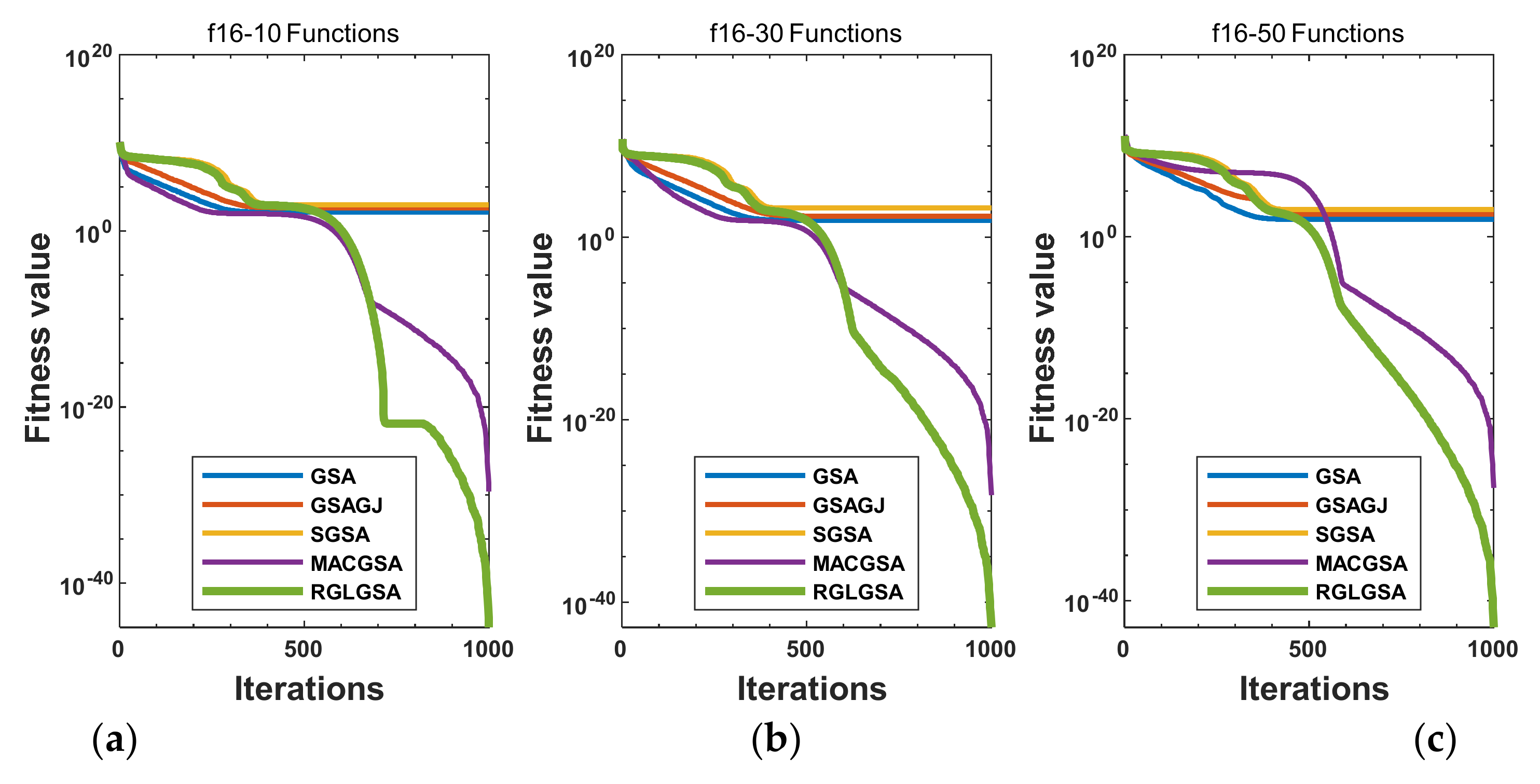
Article

Improved Gravitational Search Algorithm Based on Adaptive Strategies

1
College of Systems Engineering, National University of Defense Technology, Changsha 410073, China
2
Faculty of Electronics & Information, Xi’an Jiaotong University, Xi’an 710049, China
*
Author to whom correspondence should be addressed.
Entropy 2022, 24(12), 1826; https://doi.org/10.3390/e24121826
Submission received: 9 November 2022 / Revised: 13 December 2022 / Accepted: 13 December 2022 / Published: 14 December 2022
(This article belongs to the Section Multidisciplinary Applications)

Abstract

:
The gravitational search algorithm is a global optimization algorithm that has the advantages of a swarm intelligence algorithm. Compared with traditional algorithms, the performance in terms of global search and convergence is relatively good, but the solution is not always accurate, and the algorithm has difficulty jumping out of locally optimal solutions. In view of these shortcomings, an improved gravitational search algorithm based on an adaptive strategy is proposed. The algorithm uses the adaptive strategy to improve the updating methods for the distance between particles, gravitational constant, and position in the gravitational search model. This strengthens the information interaction between particles in the group and improves the exploration and exploitation capacity of the algorithm. In this paper, 13 classical single-peak and multi-peak test functions were selected for simulation performance tests, and the CEC2017 benchmark function was used for a comparison test. The test results show that the improved gravitational search algorithm can address the tendency of the original algorithm to fall into local extrema and significantly improve both the solution accuracy and the ability to find the globally optimal solution.

1. Introduction

With the progress of science and technology as well as the development of production and management, optimization problems cover almost all aspects of human life and production, becoming an important theoretical basis and indispensable method of modern science. The main solutions to optimization problems include traditional optimization methods and modern optimization methods. Traditional optimization methods are based on single-point optimization, and the main approaches are enumeration methods, numerical methods, and analytical methods. Modern optimization methods use swarm intelligence algorithms, inspired by the stimulation of biological evolution, that simulate the structural characteristics, evolutionary laws, thinking structures, and behavior patterns of human, natural, and other biological populations. Typical swarm intelligence algorithms include the evolutionary algorithm, artificial immune algorithm, memory algorithm, particle swarm optimization, shuffled frog leaping algorithm, cat swarm optimization, bacterial foraging optimization, artificial fish school algorithm, ant colony algorithm, and artificial bee colony algorithm. Traditional optimization methods have strict requirements for the optimization problems in practical projects, and the calculation speed is slow and the convergence is poor when solving large-scale complex problems. Often, the solution to the problem cannot be found in an acceptable time. Modern optimization methods have loose requirements for solving problems, and have good adaptability, robustness, and global search ability.
The gravitational search algorithm (GSA) was proposed by Raahedi et al. in 2009. It is a swarm intelligence global optimization algorithm that is simple to implement and achieves relatively good performance in global search and convergence. It is widely used in path planning [1,2], image classification [3,4,5], neural networks [6,7], data prediction [8,9,10], scheduling and parameter estimation [11,12,13,14,15,16,17], and other fields. However, the solution accuracy is not high, and the algorithm finds it difficult to jump out of locally optimal solutions in the later stages. To solve the shortcomings of this algorithm, scholars have improved the GSA algorithm with respect to the following three aspects: improvements to the adaptive strategy, integration with other swarm intelligence algorithms, and the introduction of other improvement strategies.
To address the first aspect, the authors of [18] proposed an adaptive GSA called SGSA in which an exponential decay model was introduced to the gravitation constant so that the algorithm can adjust the relevant parameters as required by the algorithm as the iteration proceeds. This also improves the exploration ability of the algorithm. An adaptive strategy based on population density was proposed for the distance between particles to prevent the algorithm from degenerating into random motion and to accelerate the convergence speed. The authors of [19] designed a new dynamic inertial weight and velocity position trend factor to improve the GSA, so that the inertial mass of particles has a certain trend as the iterations progress. This gives the change in position of each particle randomness and stability and gives the algorithm a certain degree of adaptability.
To address the second aspect, the authors of [20] combined the GSA with an immune algorithm, which introduces antibody diversity and immune memory characteristics into GSA and improves its global search ability. To overcome the problems of slow iterations and tendency to fall into local minima during the optimization of the standard GSA, one study [21] introduced the speed update mechanism of particle swarm optimization into the position update of GSA, combining the exploitation ability of particle swarm optimization and the exploration ability of GSA, and effectively solving the abovementioned problems. Another study [22] combined the free search differential evolution algorithm with the GSA to make full use of the exploration ability of GSA and the exploitation ability of the free search differential evolution algorithm, and to avoid the premature convergence of GSA. The authors of [23] combined the GSA with the sperm swarm optimization algorithm, which combines the advantages of both algorithms. Through testing, the hybrid method was found to have a better ability to avoid local extrema, and its convergence speed is relatively fast.
Finally, several studies have addressed the third aspect. The authors of [24] introduced a mutation operator to GSA and performed the mutation operation on particles with poor fitness values in the population. The particles were reinitialized, effectively preventing the algorithm from falling into locally optimal values, and the improved algorithm was successfully applied to an economic load scheduling problem. Another study [25] proposed the rotation GSA, which optimizes the selection of the k best in GSA by introducing a rotation operator so that unincluded particles have the opportunity to affect the motion of other particles and to enhance the exploration ability of the algorithm. The study [26] proposed a GSA based on Levy flight and chaos theory. The Levy distribution was used to improve the diversity of the population search space, and chaos search was used to strengthen candidate solutions to achieve global optimization. The authors of [27] proposed an improved GSA based on mutation strategy and reverse evaluation mechanism. The reverse learning bidirectional evaluation mechanism proposed by Tizhoosh was used to initialize and update the population so that particles were better distributed. In addition, the best individual and particles with poor fitness were cross-mutated using a mutation strategy to avoid premature convergence.
In summary, the key to improving the performance of the GSA is to balance the diversity and convergence of particles and prevent the algorithm from falling into local extreme values too early. Among the above three aspects of improvement, the adaptive strategy has a better effect and obtains the best performance. However, scholars have only used two adaptive strategies at most to improve the algorithm performance. Hence, there is room for further improvements in the algorithm’s performance. In this paper, a new adaptive GSA is proposed in which three adaptive strategies for population density, gravitation constant, and location update are used in combination to improve the optimization accuracy and convergence of the GSA. The organizational structure of this paper is as follows: Section 2 outlines the basic GSA, Section 3 introduces the three adaptive improvement strategies, Section 4 describes the idea and steps of the improved GSA and analyzes the space–time complexity and convergence performance. Finally, Section 5 evaluates the performance of the improved GSA through experiments, and Section 6 summarizes the conclusions.

2. Basic GSA

The universal GSA treats all particles as objects with mass. During the optimization process, all particles move unimpeded. Each particle is affected by the gravity of the other particles in the solution space and generates acceleration to move toward the particles with greater mass. Because the mass of the particles is related to their fitness, particles with large fitness will have greater mass. Therefore, particles with small masses will gradually approach the optimal solution in the optimization problem in the process of approaching particles with large masses. The GSA is different from other swarm intelligence algorithms. In the GSA, particles do not need to perceive the environment through environmental factors but realize information sharing through the interaction of the gravitational forces between individuals. Therefore, without the influence of environmental factors, particles can also perceive the global situation to conduct a global search in the environment, thus realizing the global optimization of the problem.
In a GSA, we assume that a D-dimensional search space contains N objects, and the position of the i-th object is
X i = ( x i 1 , x i 2 , x i 3 , ... , x i k ... x i D ) , i = 1 , 2 , ... , N
In Equation (1), x i k represents the position of the i-th object in the k-th dimension.

2.1. Inertial Mass Calculation

In the GSA, the inertial mass of each particle is directly related to the fitness value obtained from the particle location. At time t, the mass of particle X i is expressed by M i ( t ) . Because the inertial mass M is calculated according to its corresponding fitness value, the particles with larger M values are closer to the optimal solution in the solution space, and they exert a greater attraction on other objects.
Particle mass M i ( t ) is calculated according to
m i ( t ) = f i t i ( t ) w o r s t ( t ) b e s t ( t ) w o r s t ( t ) M i ( t ) = m i ( t ) j = 1 N m j ( t )
Here, f i t i ( t ) represents the fitness of particle X i , b e s t ( t ) represents the best solution at time t, w o r s t ( t ) represents the worst solution at time t, and the calculation is as follows:
b e s t ( t ) = max f i t ( t ) i { 1 , 2 , ... , N } w o r s t ( t ) = min f i t ( t ) i { 1 , 2 , ... , N }
It can be seen from Equation (2) that m i ( t ) normalizes the fitness of particles to the range [0, 1] and then takes its proportion in the total mass as the mass M i ( t ) of the particles.

2.2. Gravitational Calculation

At time t, the calculation of the gravitational force of object j subjected to object i in the k-th dimension is as follows:
F i j k ( t ) = G ( t ) M a i ( t ) × M a j ( t ) R i j ( t ) + ε ( x j k ( t ) x i k ( t ) ) ,
where ε represents a very small constant, Maj(t) represents the inertial mass of the action object j, and Mai(t) represents the inertial mass of the action object i. Furthermore, G(t) represents the constant of universal gravitation transformed over time, where its size is related to the number of iterations, and its calculation is
G ( t ) = G 0 × e α t / T .
In Equation (5), G0 represents the value of G at time t0, where G0 = 100, α = 20, and T is the maximum number of iterations. Finally, R i j ( t ) represents the Euclidean distance between objects X i and X j , and is calculated as
R i j ( t ) = X i ( t ) - X j ( t ) 2 .
At time t, the force acting on X i in the k-th dimension is equal to the sum of the forces exerted on it by all other particles around as follows:
F k i ( t ) = j = 1 , j i N r a n d F j i j k ( t ) .

2.3. Location Update

When a particle is subjected to the gravitational action of other particles, it will generate acceleration. According to the gravity calculated in Equation (7), the acceleration obtained by object i in the k-th dimension is the ratio of its force to inertial mass. The calculation is as follows:
α i k ( t ) = F i k ( t ) M i ( t ) .
In each iteration, the algorithm updates the speed and position of object i according to the calculated acceleration. The update method is
v i k ( t + 1 ) = r a n d i × v i k + α i k ( t ) ,
x i k ( t + 1 ) = x i k ( t ) + v i k ( t + 1 ) .
The basic GSA implementation steps are as follows:
  • Initialize the position and acceleration of all particles in the algorithm, and set the number of iterations and parameters.
  • Calculate the fitness value for each particle, and update the gravitation constant according to the formula.
  • The mass of each particle is calculated according to the calculated fitness value, and the acceleration of each particle is calculated using Equations (2)–(8).
  • Calculate the speed of each particle according to Equation (9) and then update the particle position according to Equation (10).
  • If the termination condition is not met, return to step 2; otherwise, output the optimal solution of the algorithm.

3. Adaptive Strategies

3.1. Adaptive Population Density Strategy

The distance between particles in the basic GSA is the Euclidean distance. Through a large number of experiments in [18], it was found that a constant fixed distance is better than the Euclidean distance, but the fixed distance value has obvious shortcomings: First, when the population is divided, the distance between particles is large and the interaction force is very small, and hence, the GSA degenerates into random motion. Second, when the population is dense, the distance between particles is very small, and the interaction force is very large. The particles in the algorithm will oscillate at a high frequency near the optimal solution and reduce the convergence speed. The population density is an indicator for evaluating the distance between particles, and it is the median of the average distance of all particles in the population. A smaller population density means the population is more concentrated; by contrast, a higher population density means the population is more dispersed. To solve the above two issues, balance the exploration and exploitation abilities of the algorithm, adjust the search ability of the algorithm, and propose an adaptive strategy based on population density, we dynamically adjust the distance between particles according to the GSA population density. That is, when the population density is relatively large, the population is relatively dispersed, reducing the particle distance between populations, promoting information exchange between particles, and preventing random movement between particles. When the population density value is small, the population is dense. We hence increase the distance between population particles appropriately to speed up the convergence of the algorithm. The calculation of population density δ is as follows:
δ = 1 N i = 1 N d i s i ,
where N is the number of particles, D is the dimensionality of the particles, and disi is the average distance between the i-th particle and all other particles, calculated as follows:
dis i = 1 N - 1 j = 1 , j i N k = 1 D ( x i k x j k ) 2 .
The gravitational force calculated in the basic universal GSA is modified as follows:
F i j k ( t ) = G ( t ) M a i ( t ) × M a j ( t ) R i j Rp ( δ ) ( t ) + ε ( x j k ( t ) x i k ( t ) ) .
The calculation of Rp ( δ ) is
Rp ( δ ) = R p min + ( R p max R p min ) e 1 1 / δ δ < 1 R p min + ( R p max R p min ) e 1 δ δ 1 ,
where Rpmax and Rpmin are the maximum and minimum values of the given fixed distance, respectively, and δ is the population density.

3.2. Adaptive Gravitational Constant Strategy

Gravitational constant G is an important variable that transforms over time. Its change directly affects the magnitude of resultant force and acceleration, as well as determines the current step size and convergence speed of particles in the algorithm. The reasonable selection of parameters G0 and α plays an important role in the size of the iterative steps in the algorithm and determines whether the algorithm can jump out of local optima and determine the direct factor of optimal accuracy. If the original gravitational constant decreases quickly at the beginning of the algorithm, the algorithm can converge quickly, but it also tends to fall into the local optima and is difficult to jump out. To improve the exploration ability of the algorithm, prevent the algorithm from falling into locally optimal solutions, and improve the accuracy of the solution, an adaptive strategy for the universal gravitational constant is proposed. The adaptive gravitational constant G is expressed as follows:
G ( t ) = G 0 1 + e α ( t t c ) / T 0 t c < T
Here, G 0 is the initial value of the universal gravitational constant, α is the parameter of the decay rate, T is the total number of iterations, and tc is a constant value in the interval [0, T).

3.3. Adaptive Location Update Strategy

A position in the basic GSA is updated according to the current speed of the algorithm and the position in the last iteration. In each iteration, if the current update speed of particles is small, the change in position will also be small, the convergence ability of the algorithm will be reduced, and the algorithm will tend to fall into local extrema. By contrast, if the current update speed of particles is too large, the change in position will also increase, and the algorithm will move far from the global optimum. To address these defects, the improved strategy in [3] is adopted in this study to make the position of the particles change with respect to the iterative evolution. In the early stages of the algorithm, each particle moves with a large step size so that the algorithm can quickly converge to the vicinity of the optimal solution; in the later stages of the algorithm, the particle update step is smaller, and the particle depth search is near the optimal value. The expression of the adaptive position update is
x i k ( t + 1 ) = α × x i k ( t ) + β × v i k ( t + 1 ) ,
where α is calculated by
α = e ( dim * ( t / T max ) ω )
and β is calculated by
β = 1 t T max + b e t a r n d ,
where dim is the dimension; ω is an integer in the range [1, 50]; T is the current number of iterations of the algorithm; Tmax is the maximum number of iterations set for the algorithm; and betarnd is the random number generated by the [0, 1] beta distribution. The range of α is (0, 1) and the range of β is (0, 1).

4. Improved GSA Based on Adaptive Strategies

4.1. Basic Concept

To improve the low solution accuracy and difficulty of jumping out of the locally optimal solutions of conventional GSA, the parameters for the distance between particles, gravitational constant, and position update in GSA are improved using adaptive strategies to strengthen the information interaction between particles and improve the exploration and exploitation capabilities of the algorithm.
The steps of the proposed algorithm are as follows.
  • Step 1: The proposed adaptive GSA is initialized to generate the initial particle swarm. Set the size of algorithm particle swarm N and the maximum number of iterations NCMax, search space dimension XDim, maximum distance Rpmax, minimum distance Rpmin, gravitational constant, attenuation rate, constant value, and other parameter values.
  • Step 2: Check the particle boundary in the population, and calculate the fitness value of particles in the population.
  • Step 3: Use Equation (3) to calculate best(t) and worst(t).
  • Step 4: The inertial mass Mi(t) of the particles is obtained according to best(t), worst(t), and Equation (2).
  • Step 5: Update the gravitational constant G according to Equation (15).
  • Step 6: Calculate the distance between particles according to Equations (6), (11), and (14).
  • Step 7: Calculate the gravitational and resultant forces around particles according to Equation (13).
  • Step 8: Calculate the acceleration of the particles according to Equation (8).
  • Step 9: Update particle speeds and positions according to Equations (9) and (16)–(18).
  • Step 10: Return to the iteration cycle in step 2 until the number of cycles or accuracy requirements are met.
  • Step 11: Exit the loop and output the algorithm results.

4.2. Temporal and Spatial Complexity Analyses

4.2.1. Time Complexity Analysis

The time complexity of the algorithm is the time spent executing the algorithm, which is equal to the cumulative number of times the algorithm performs basic operations such as addition, subtraction, multiplication, division, and comparison. Assuming that the particle swarm size of the proposed adaptive GSA is N, the time complexity of the algorithm is analyzed according to the steps of the algorithm execution using the method in [28].
In step 1, the initialization of the particle swarm of the proposed adaptive GSA requires N operations, and the initialization operations of the other parameters are a constant; thus, the time complexity of step 1 is O (N).
In step 2, the particle boundary check requires N operations, the fitness calculation requires N operations, and hence, the time complexity of step 2 is O(N) + O(N).
In step 3, it takes one operation to calculate the best fitness value best(t) and one operation to calculate the worst fitness value worst(t), and hence, the time complexity of step 3 is O(1) + O(1).
Calculating the inertial mass Mi(t) of particles in step 4 requires N operations; thus, the time complexity of step 4 is O(N).
Updating the gravitational constant G in step 5 requires one operation; thus, the time complexity of step 5 is O(1).
In step 6, calculating the average distance of all particles requires N × (N − 1) operations, calculating the population density requires one operation, and calculating the particle distance requires one operation, and hence, the time complexity of step 6 is O(N × (N − 1)) + O(1) + O(1).
In step 7, calculating the gravity of particles in the population requires N operations, and calculating the resultant force of particles in the population requires N operations; thus, the time complexity of step 7 is O(N) + O(N).
In step 8, calculating particle acceleration requires N operations, and calculating particle velocity requires N operations, and hence, the time complexity of step 8 is O(N) + O(N).
Updating particle positions in step 9 requires N operations; thus, the time complexity of step 9 is O(N).
In step 10, evaluating the termination condition requires one comparison operation, and terminating the algorithm requires one assignment operation; thus, the time complexity of step 10 is O(1) + O(1).
After the above steps, the proposed adaptive GSA performs NCmax iterations. The time complexity the proposed adaptive GSA after the maximum number of iterations is O(NCmax × (N × N)).

4.2.2. Spatial Complexity Analysis

Space complexity is a measure of the storage space occupied by the algorithm during execution. Assume that the population size of the proposed adaptive GSA is N, the number of iterations of the algorithm is NCmax, and the dimensionality of the optimization function is D. We perform spatial complexity analysis according to the steps of algorithm execution. In the proposed adaptive GSA, X [N] [D] is used to store the value of initialization independent variable, Y [1] [N] is used to store the fitness value of initialization function, Xm [1] [N] is used to store the inertial mass value of population particles, Xd [1] [N] is used to store the average distance between population particles, Xf [N] [D] is used to store the resultant force value around each particle in the population, Xa [N] [D] is used to store the acceleration value of each particle in the population, and Xv [N] [D] is used to store the velocity value of each particle in the population. Therefore, the space complexity of the whole GSA based on adaptive strategy improvement is 4 × O(N × D).

4.2.3. Analysis of Algorithm Convergence

The convergence of the proposed adaptive GSA is proven using the contraction mapping theorem. For the relevant concepts and theorems in space compression theory, we refer readers to the definitions in [28].
Theorem 1.
As the time tends to infinity, the proposed adaptive GSA is convergent.
Proof:
The state of the proposed adaptive GSA in the optimization process is represented by set X. The mutual transformation of states in set X is actually the embodiment of the whole optimization process of the proposed adaptive GSA. Therefore, the optimization process of the proposed adaptive GSA is a self-mapping process. If f is an optimization process mapping from X to X, then X k + 1 = f ( X k ) . Suppose ρ : X × X R is the distance between two points in metric space ( X , ρ ) and x n is any optimization sequence in ( X , ρ ) . □
The proposed adaptive GSA is a continuous iterative process. Under the action of gravity, individuals in the algorithm attract each other, forcing small mass individuals to constantly move to larger mass individuals to determine the optimal solution X . Therefore, in metric space ( X , ρ ) , for any ε , there exists an N, where n > N, such that ρ ( x n , X ) < ε is true. According to its definition, the optimization sequence x n converges to X . Moreover, x n is a Cauchy sequence, and ( X , ρ ) is a complete metric space. Let ε be a random number in the range [0, 1]. Since the proposed adaptive GSA is a continuous optimization process, individuals are constantly approaching the optimal value, and hence, it is a convergent process. Then, there must be ρ ( f ( x ) , f ( y ) ε ρ ( x , y ) in the metric space ( X , ρ ) , and f is a compression mapping. According to Theorem 4.2 in [28], x = lim k f * ( x 0 ) is true, where x X is the only fixed point in the compressed mapping f . Hence, the proposed adaptive GSA is convergent, and Theorem 1 is proven.

5. Experimental Analysis

5.1. Performance of the Algorithm Improvement Strategies

This section evaluates and analyzes the combinations of the three adaptive improvement strategies in the algorithm: the adaptive population density strategy, adaptive gravitational constant strategy, and adaptive location update strategy. For the convenience of description, we refer to the GSA based on the adaptive population density strategy as the RGSA. Similarly, we call the GSA based on the adaptive gravitational constant strategy the GGSA, and the GSA based on the adaptive position strategy is called the LGSA. The GSA based on the adaptive population density and gravity constant strategies is the RGGSA, the GSA based on the adaptive population density and location update strategies is the RLGSA, the GSA based on the adaptive gravity constant and position update strategies is the GLGSA, and the GSA based on all three adaptive population density, gravity constant, and location update strategies is the RGLGSA. In the experiment, we tested the convergence of the basic GSA and the GSA with the seven different adaptive strategies on benchmark functions f1 to f15.

5.1.1. Test Functions

Table 1 lists the test functions. Among the 15 standard test functions, the minimum value 0.397887 is obtained at points ( π , 12.275), ( π , 2.275), and (9.42478, 2.475), and the other functions obtain the minimum value 0 at point (0, 0, ..., 0). The functions f1, f2, f3, f7, f8, f10, and f13 are unimodal test functions. These functions only have one globally optimal solution, and are mainly used to test the solution accuracy and development ability of the algorithm. Functions f4, f5, f6, f9, f11, f12, f14, and f15 are multimodal test functions. These functions have many local extrema. The GSA is prone to premature convergence or falling into local extrema. To determine the optimal values for these test functions, the algorithm must have the ability to jump out of local extrema, avoid premature convergence, and have strong global exploration ability.

5.1.2. Data Analysis

We set the initial parameters of the algorithms as follows: for the basic GSA, G0 was 100 and α was 20; for RGSA: G0 was 100, α · was 20, tc was T/4, Rpmax was 1.5, and Rpmin was 0.5; for GGSA: G0 was 50 and α · was 30; for SGSA: G0 was 100, α was 20, and ω was 10. The parameter settings of the other GSAs were consistent with those of the previous three GSAs. The population size for all algorithms was 50, the number of algorithm iterations was 1000, the test dimensions were 30 and 50, functions f6 and f11 were two-dimensional tests, and the number of independent algorithm runs was 30.
The following observations can be inferred from the simulation test results of Table 2, Table 3, Table 4, Table 5, Table 6, Table 7, Table 8, Table 9, Table 10, Table 11, Table 12, Table 13, Table 14, Table 15 and Table 16.
First, the results of the RGSA, GGSA, and LGSA on the test functions are better than those of the GSA. The results show that the three adaptive strategies of population density, gravitational constant, and location update can effectively improve the performance of the GSA. The detailed analysis is as follows. The result of the GGSA is inferior to those of the RGSA and LGSA, but superior to that of the GSA. This shows that although the adaptive gravitational constant strategy is inferior to the crowd density and location update strategy in improving the performance of the GSA, it also improves the performance of the GSA to a certain extent because it helps to improve the iteration step size and convergence speed. The result of the RGSA is much better than that of the GSA, which indicates that the adaptive population density strategy dynamically adjusts the distance between particles according to the population density in the evolution process and better balances the exploration and mining capabilities of the algorithm, thus improving the search capability of the algorithm. The LGSA is not only better than the GSA, but also better than the GGSA and RGSA, which shows that the location update strategy plays the largest role in improving the performance of the GSA and reflects that the balance of location and speed between individuals is the key to ensuring the good solution quality of a swarm intelligence algorithm.
Second, the results of the RGGSA, RLGSA, and GLGSA on the test function are better than those of the RGSA, GGSA, and LGSA. The results show that the combination of two of the three adaptive strategies proposed in this paper can effectively improve the performance of the GSAs using a single strategy. The result of the GLGSA is better than that of the RGGSA, but it is also inferior to that of the RLGSA, which indicates that the better single improvement strategy still has a higher performance advantage in the combined improvement strategy. The test result of the RGLGSA is higher than those of the RGGSA, RLGSA and GLGSA. The results shows that the RGSGSA, which combines the three strategies, leverages the advantages of the RGSA, GGSA, and LGSA, making the advantages more effective in the search process and achieving the best solution performance.

5.2. Comparison and Analysis of Algorithm Test Results

To fully evaluate the overall performance of the adaptive GSA proposed in this paper (RGLGSA), we selected the following classic and efficient GSA algorithms: the weight-based GSA (GSAGJ) [29], SGSA [18], and multipoint adaptive constraint-based gravitation improved algorithm (MACGSA) [19]. A comparative analysis of simulation tests was performed using 16 benchmark test functions of the CEC2017 benchmark. In the experiment, we tested the convergence of the basic GSA and the four comparison algorithms in 10, 30, and 50 dimensions.

5.2.1. Test Function

In this study, 16 benchmark test functions of CEC2017 were selected to test the effectiveness of the proposed algorithm. Table 17 lists each test function. Among the 16 test functions, f19 and f23 take the minimum value 0 at point (1, 1, ..., 1), f29 and f30 take the minimum value 0 at point (−1, −1, ..., −1), and the other functions take the minimum value 0 at point (0, 0, ..., 0). Functions f16, f17, f18, f24, and f25 are multidimensional unimodal reference functions, whereas f19–f23 and f26–f31 are multidimensional multimodal reference functions.

5.2.2. Data Analysis

To prevent errors caused by accidental factors and to ensure objectivity and fairness of the evaluation, in the experiment, the five algorithms were independently run 30 times and were iterated 1000 times in the same environment. The other parameter settings of the algorithms were consistent with those listed in Section 5.1.
The CEC2017 benchmark test function simulation results in Table 18, Table 19, Table 20, Table 21, Table 22, Table 23, Table 24, Table 25, Table 26, Table 27, Table 28, Table 29, Table 30, Table 31, Table 32 and Table 33 reveal the following.
First, for the unimodal functions f16, f18, f24, and f25, both the RGLGSA and MACGSA have high accuracy. Under the same number of dimensions, the optimization accuracy of the RGLGSA proposed in this paper is significantly higher than those of the GSA, GSAGJ, SGSA, and MACGSA. With different dimensions, as the dimensions increase, the solution accuracy of the five algorithms gradually decreases, but the solution accuracy of the RGLGSA is still higher than those of the GSA, GSAGJ, SGSA, and MACGSA. For function f17, both the RGLGSA and MACGSA have very high accuracy. Under the same number of dimensions, the optimization accuracy of the RGLGSA is superior to those of the other four algorithms. As the dimensions increase, the solution accuracy of the GSA, GSAGJ, and SGSA decrease gradually, with an obvious trend. The solution accuracies of the RGLGSA and MACGSA increase gradually, but the solution accuracy of the RGLGSA is still higher than that of the other four algorithms.
For the multimodal functions f19, f29, and f30, the four algorithms all become trapped in the local extrema, with little difference in solution accuracy. For functions f20, f21, f26, f27, and f28, the RGLGSA and MACGSA find the globally optimal solution 0, but other algorithms cannot. For function f22, when the dimensions are 10, the RGLGSA and MACGSA can find the global optimal solution 0; when the dimensions are high, only the RGLGSA can find the globally optimal solution 0. For function f23, when the dimensions are 10, the SGSA has a higher precision, and when the dimensions are 30 and 50, the RGLGSA has the highest precision. For function f31, under the same number of dimensions, the optimization accuracy of the RGLGSA is significantly higher than those of the other algorithms. As the dimensions increase, the solution accuracies of the GSA, GSAGJ, and SGSA decrease gradually. When the dimensions reach 50, the solution accuracies of the MACGSA and RGLGSA decrease significantly.
The comparison and test results of the above algorithms reveal that, compared with other classical and efficient improved GSAs, the RGLGSA has a relatively stable overall search ability on unimodal functions and multimodal functions. Moreover, it has a high convergence accuracy.

5.2.3. Curve Analysis

Figure 1, Figure 2, Figure 3, Figure 4, Figure 5, Figure 6, Figure 7, Figure 8, Figure 9, Figure 10, Figure 11, Figure 12, Figure 13, Figure 14, Figure 15 and Figure 16 show the convergence curves of the RGLGSA, basic GSA, and the comparison GSAs. The convergence curves of the unimodal functions reveal that there is little difference between the convergence speed of the five algorithms in the first 500 generations. After 500 generations, the GSA, GSAGJ, and SGSA converge to the local extreme values and stop searching. The MACGSA and RGLGSA do not fall into the local extreme values, but continue to evolve. However, the convergence speed of the RGLGSA is faster than that of the MACGSA, and the obtained value is better.
For multimodal functions f19, f29 and f30, in the first 400 iterations, the convergence speed of the RLSGSA is roughly the same as those of the other four algorithms. Because of the characteristics of the functions and algorithms, after 400 iterations, the five algorithms converge to a local extremum, and the differences between the solutions obtained by the algorithms are not significant. For multimodal functions f20, f21, f27, and f28, GSA, GSAGJ, and SGSA converge to the local extreme value after a certain number of iterations and stop searching. The MACGSA and RGLGSA do not fall into the local extreme value but continue to evolve to find the globally optimal solution 0. However, the RGLGSA converges faster than the MACGSA. For multimodal function f22, in the first 500 iterations, the convergence speed of the RLSGSA is roughly the same as that of the other four algorithms. After 500 generations, the other four algorithms fall into local extrema, and the RLSGSA finds the global optimal solution 0 after about 650 generations. For multimodal function f31, in the first 300 iterations, the convergence rates of the five algorithms are similar. After 300 generations, the GSA, GSAGJ, and SGSA have stopped iterative evolutions, and the algorithms have fallen into locally optimal solutions. The MACGSA and RGLGSA continue to evolve after 600 generations, and finally, the MACGSA finds a better solution at a faster speed. For multimodal function f23, in 10 dimensions, the GSA and GSAGJ stop iterations after about 400 generations. After 400 generations, the convergence speed of the RGLGSA is faster than that of the SGSA and MACGSA. At 30 and 50 dimensions, the convergence accuracies of the five algorithms are not high. The GSAGJ has the fastest convergence speed, followed by the RGLGSA, but the convergence accuracy of the RGLGSA is higher than that of the GSAGJ. For multimodal function f26, the convergence speed of the MACGSA is higher before generation 500, the convergence speed of the RGLGSA is higher after generation 500, and the optimal value is obtained around generation 880. As a whole, the convergence speed of the RGLGSA is higher than those of the other comparison GSAs.
In general, compared with other GSA methods, the proposed adaptive GSA based on the adaptive strategies of population density, gravitational constant, and location update has a greatly improved optimization accuracy and stability, and performs well with respect to convergence.

6. Conclusions

In this paper, we proposed an improved GSA that is based on adaptive strategies. To address the shortcomings of the basic GSA, this algorithm introduces adaptive strategies based on crowd density, the gravitational constant, and location update into the basic universal GSA simultaneously. Moreover, it dynamically adjusts the distance between particles and the step size of the particle iteration, strengthens the information exchange between particles, and greatly increases the diversity of particles in the population. Therefore, it can effectively overcome the disadvantages of the basic GSA, which tends to fall into local extreme values. The simulation results show that the improved algorithm is superior to other classically improved GSAs in terms of search accuracy, convergence speed, stability, and other factors. It hence is an effective extension to the algorithm.
No Free Lunch Theory is a very important theorem in the field of optimization research, which reflects that no optimization algorithm can outperform other algorithms in average performance on all optimization problems. The improved algorithm in this paper also has this problem, and the experimental analysis cannot fully cover many optimization problems, which is convincing. The future research direction is mainly to optimize the overall performance of the algorithm, so that the performance of the improved algorithm is better than that of other algorithms on as many optimization problems as possible.

Author Contributions

Conceptualization, Z.Y.; methodology, Z.Y.; software, Z.Y.; validation, Y.C.; formal analysis, Z.Y.; investigation, G.L.; resources, Y.C.; data curation, G.L.; writing—original draft preparation, Y.C.; writing—review and editing, Z.Y.; visualization, G.L.; supervision, Y.C.; project administration, Y.C. and G.L.; funding acquisition, Z.Y. All authors have read and agreed to the published version of the manuscript.

Funding

This research received no external funding.

Institutional Review Board Statement

Not applicable.

Data Availability Statement

Data is available upon reasonable request from the author.

Conflicts of Interest

The authors declare no conflict of interest.

References

  1. Das, P.K.; Behera, H.S.; Jena, P.K.; Panigrahi, B.K. An intelligent multi-robot path planning in a dynamic environment using improved gravitational search algorithm. Int. J. Autom. Comput. 2021, 18, 1032–1044. [Google Scholar] [CrossRef]
  2. Xu, H.; Jiang, S.; Zhang, A. Path planning for unmanned aerial vehicle using a Mix-strategy-based gravitational search algorithm. IEEE Access. 2021, 9, 57033–57045. [Google Scholar] [CrossRef]
  3. Wang, Y.; Tan, Z.P.; Chen, Y.C. An adaptive gravitational search algorithm for multilevel image thresholding. J. Supercomput. 2021, 77, 10590–10607. [Google Scholar] [CrossRef]
  4. Tan, Z.; Zhang, D. A fuzzy adaptive gravitational search algorithm for two-dimensional multilevel thresholding image segmentation. J. Ambient Intell. Hum. Comput. 2020, 11, 4983–4994. [Google Scholar] [CrossRef]
  5. Alenazy, W.M.; Alqahtani, A.S. An automatic facial expression recognition system employing convolutional neural network with multi-strategy gravitational search algorithm. IETE Tech. Rev. 2022, 39, 72–85. [Google Scholar] [CrossRef]
  6. García-Ródenas, R.; Linares, L.J.; López-Gómez, J.A. Memetic algorithms for training feedforward neural networks: An approach based on gravitational search algorithm. Neural. Comput. Appl. 2021, 33, 2561–2588. [Google Scholar] [CrossRef]
  7. Nagra, A.A.; Alyas, T.; Hamid, M.; Tabassum, N.; Ahmad, A. Training a feedforward neural network using hybrid gravitational search algorithm with dynamic multiswarm particle swarm optimization. BioMed Res. Int. 2022, 2022, 2636515. [Google Scholar] [CrossRef] [PubMed]
  8. Nobahari, H.; Alizad, M.; Nasrollahi, S. A nonlinear model predictive controller based on the gravitational search A nonlinear model predictive controller based on the gravitational search algorithm. Optim. Control Appl. Meth. 2021, 42, 1734–1761. [Google Scholar] [CrossRef]
  9. Zhang, X.Q.; Wu, X.L.; Zhu, G.Y.; Lu, X.; Wang, K. A seasonal Arima model based on the gravitational search algorithm (GSA) for runoff prediction. Water Supply 2022, 22, 6959–6977. [Google Scholar] [CrossRef]
  10. Singh, A.; Singh, N. Gravitational search algorithm-driven missing links prediction in social networks. Concurr. Computat. Pract. Experience 2022, 34, e6901. [Google Scholar] [CrossRef]
  11. Younes, Z.; Alhamrouni, I.; Mekhilef, S.; Reyasudin, M. A memory-based gravitational search algorithm for solving economic dispatch problem in micro-grid. Ain. Shams Eng. J. 2021, 12, 1985–1994. [Google Scholar] [CrossRef]
  12. Cao, C.W.; Zhang, Y.; Gu, X.S.; Li, D.; Li, J. An improved gravitational search algorithm to the hybrid flowshop with unrelated parallel machines scheduling problem. Int. J. Prod. Res. 2021, 59, 5592–5608. [Google Scholar] [CrossRef]
  13. Habibi, M.; Broumandia, A.; Harounabadi, A. An Intelligent Traffic Light Scheduling Algorithm by using fuzzy logic and gravitational search algorithm and considering emergency vehicles. Int. J. Nonlinear Anal. Appl. 2021, 11, 475–482. [Google Scholar]
  14. Thakur, A.S.; Biswas, T.; Kuila, P. Binary quantum-inspired gravitational search algorithm-based multi-criteria scheduling for multi-processor computing systems. J. Supercomput. 2021, 77, 796–817. [Google Scholar] [CrossRef]
  15. He, J.F.; Wang, T.; Li, Y.J.; Deng, Y.L.; Wang, S.B. Dynamic chaotic gravitational search algorithm-based kinetic parameter estimation of hepatocellular carcinoma on F-18-FDG PET/CT. BMC Med. Imaging 2022, 22, 20. [Google Scholar] [CrossRef]
  16. Enikeeva, L.V.; Potemkin, D.I.; Uskov, S.I.; Snytnikov, P.V.; Enikeev, M.R.; Gubaydullin, I.M. Gravitational search algorithm for determining the optimal kinetic parameters of propane pre-reforming reaction. React. Kinet. Mech. Cat. 2021, 132, 111–122. [Google Scholar] [CrossRef]
  17. Ismail, A.M.; Mohamad, M.S.; Abdul Majid, H.A.; Abas, K.H.; Deris, S.; Zaki, N.; Mohd Hashim, S.Z.; Ibrahim, Z.; Remli, M.A. An improved hybrid of particle swarm optimization and the gravitational search algorithm to produce a kinetic parameter estimation of aspartate biochemical pathways. Biosystems 2017, 162, 81–89. [Google Scholar] [CrossRef]
  18. Zhenkai, X. Modification and Application of Gravitational Search Algorithm. Master’s Thesis, University of Shanghai for Science & Technology, Shanghai, China, 2014. [Google Scholar]
  19. Yuhao, X. The Improvement and Application of Gravitational Search Algorithm. Master’s Thesis, Henan University, Kaifeng, China, 2018. [Google Scholar]
  20. Jing, Y.; Fang, L.; Peng, D. Research and simulation of the gravitational search algorithms with immunity. Acta Armamentarii 2012, 33, 1528–1533. [Google Scholar]
  21. Xiaogang, L.I.U.; Ouyang, Z. Application of improved gravitational search algorithm in function optimization. J. Shenyang Univ. Technol. 2021, 43, 193–197. [Google Scholar]
  22. Liu, Y.; Ma, L. Improved gravitational search algorithm based on free search differential evolution. J. Syst. Eng. Electron. 2013, 24, 690–698. [Google Scholar] [CrossRef]
  23. Shehadeh, H.A. A hybrid sperm swarm optimization and gravitational search algorithm (HSSOGSA) for global optimization. Neural. Comput. Appl. 2021, 33, 11739–11752. [Google Scholar] [CrossRef]
  24. Huang, Y.; Wang, J.R.; Guo, F. Economic load dispatch using improved gravitational search algorithm. In Proceedings of the 2016 2nd ISPRS International Conference on Computer Vision in Remote Sensing (CVRS), Xiamen, China, 28–30 April 2015; Volume 9901. [Google Scholar]
  25. Wang, R.P.; Su, F.; Hao, T.G.; Li, J.L. RGSA: A new improved gravitational search algorithm. In Proceedings of the 2016 3rd International Conference on Modelling, Simulation and Applied Mathematics (MSAM), Shanghai, China, 22–23 July 2018; Volume 160, pp. 202–207. [Google Scholar]
  26. Rather, S.A.; Bala, P.S. Lévy flight and chaos theory-based gravitational search algorithm for mechanical and structural engineering design optimization. Open Comput. Sci. 2021, 11, 509–529. [Google Scholar] [CrossRef]
  27. Chen, X.; Shuo, L.I.U. Improvement of universal gravitation search algorithm based on reverse evaluation mechanism. J. Wuhan Polytech. Univ. 2016, 35, 60–63. [Google Scholar]
  28. Teng, F. Research on Improved Artificial Fish Swarm Algorithm and Its Application in Logistics Location Optimization. Ph.D. Thesis, Tianjin University, Tianjin, China, 2016. [Google Scholar]
  29. Xu, Y.; Wang, S. Enhanced version of gravitational search algorithm: Weighted GSA. Comput. Eng. Appl. 2011, 47, 188–192. [Google Scholar]
Figure 1. Convergence curves of function f16: (a) 10 dimensions, (b) 30 dimensions, and (c) 50 dimensions.
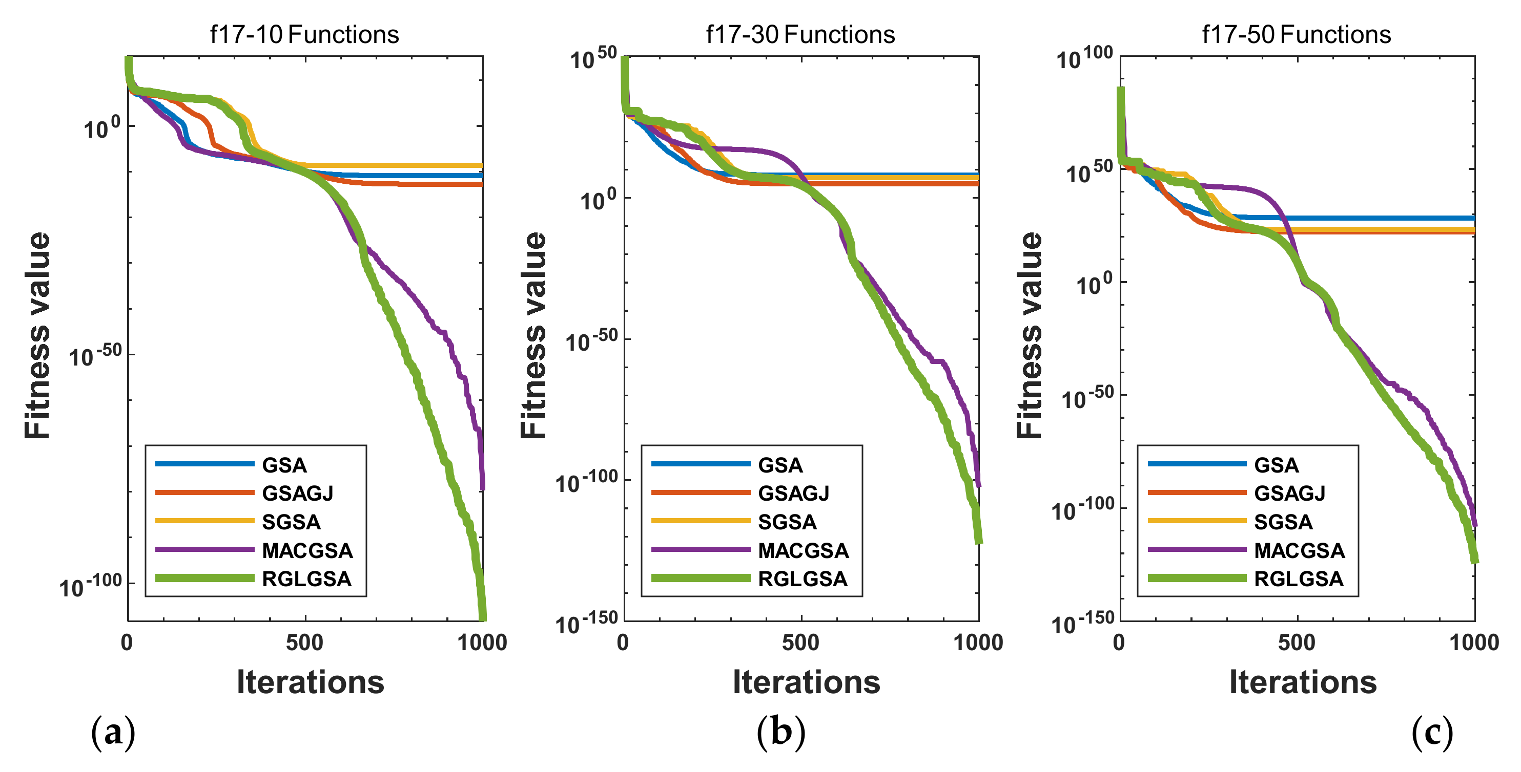
Entropy 24 01826 g001
Figure 2. Convergence curves of function f17: (a) 10 dimensions, (b) 30 dimensions, and (c) 50 dimensions.
Entropy 24 01826 g002
Figure 3. Convergence curves of function f18: (a) 10 dimensions, (b) 30 dimensions, and (c) 50 dimensions.
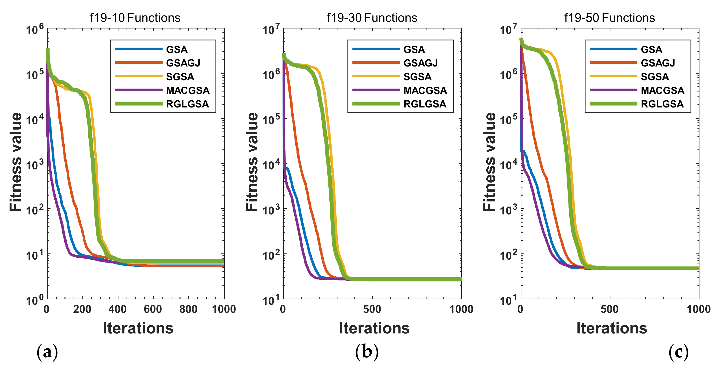
Entropy 24 01826 g003
Figure 4. Convergence curves of function f19: (a) 10 dimensions, (b) 30 dimensions, and (c) 50 dimensions.
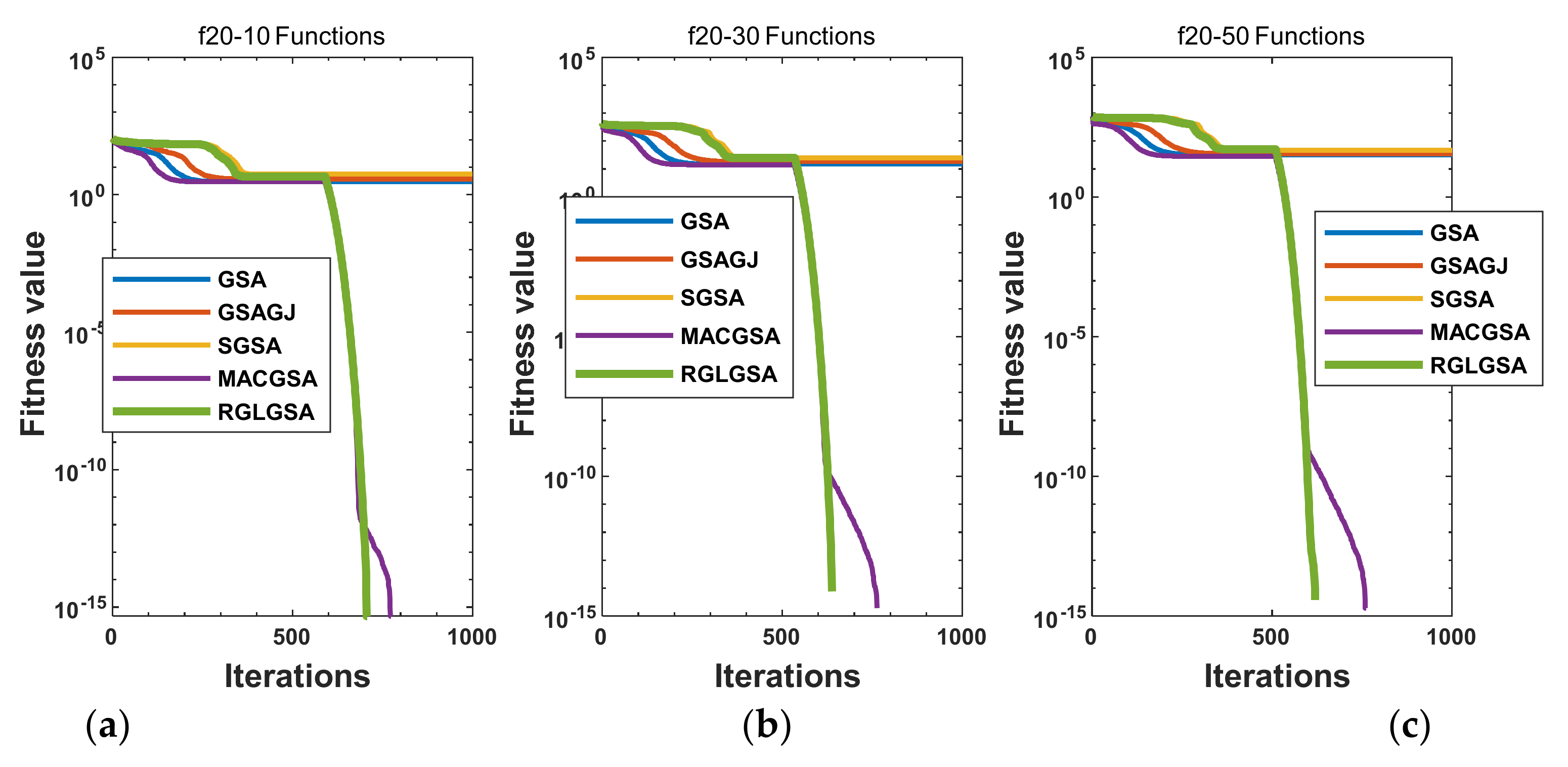
Entropy 24 01826 g004
Figure 5. Convergence curves of function f20: (a) 10 dimensions, (b) 30 dimensions, and (c) 50 dimensions.
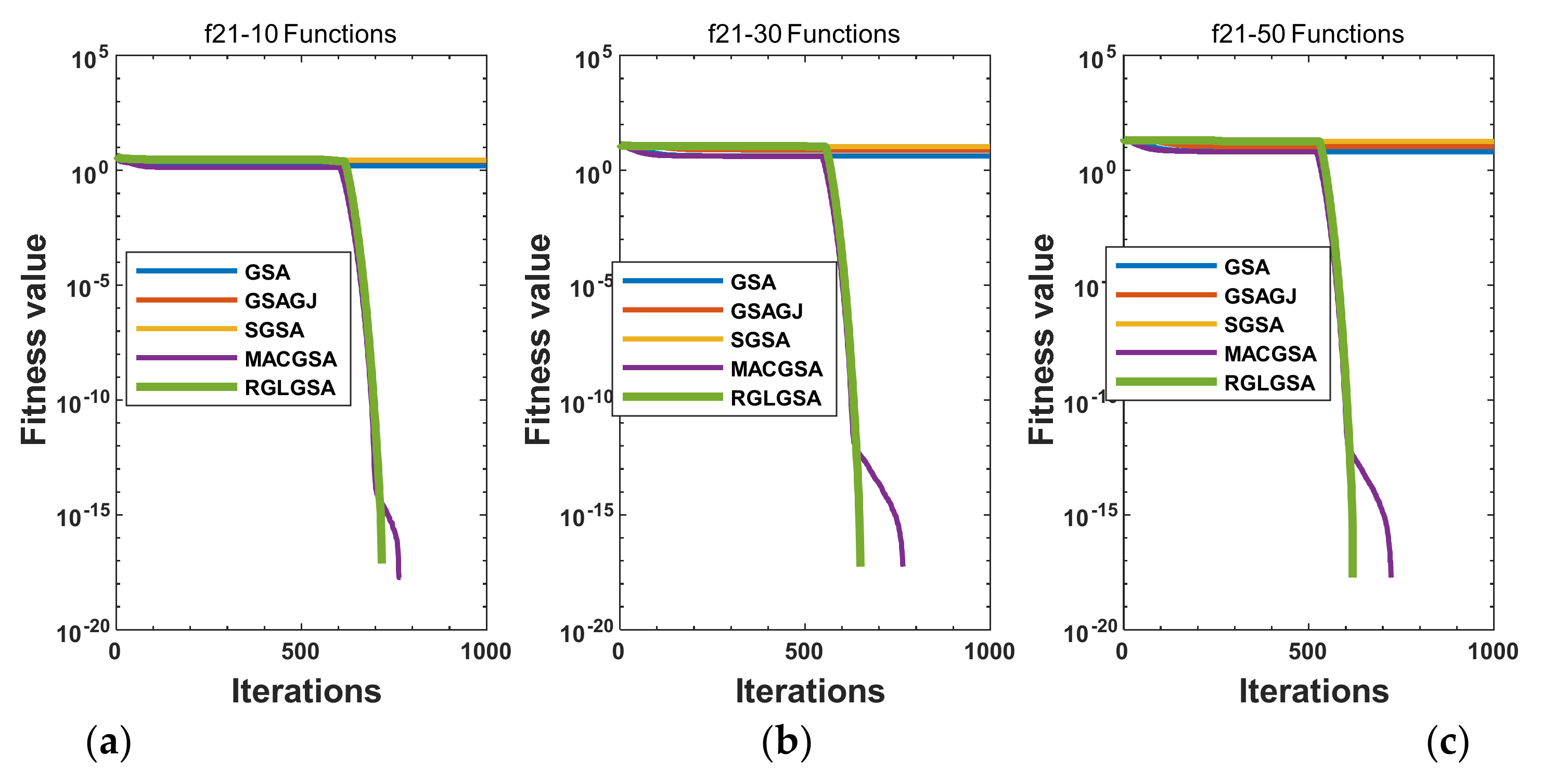
Entropy 24 01826 g005
Figure 6. Convergence curves of function f21: (a) 10 dimensions, (b) 30 dimensions, and (c) 50 dimensions.
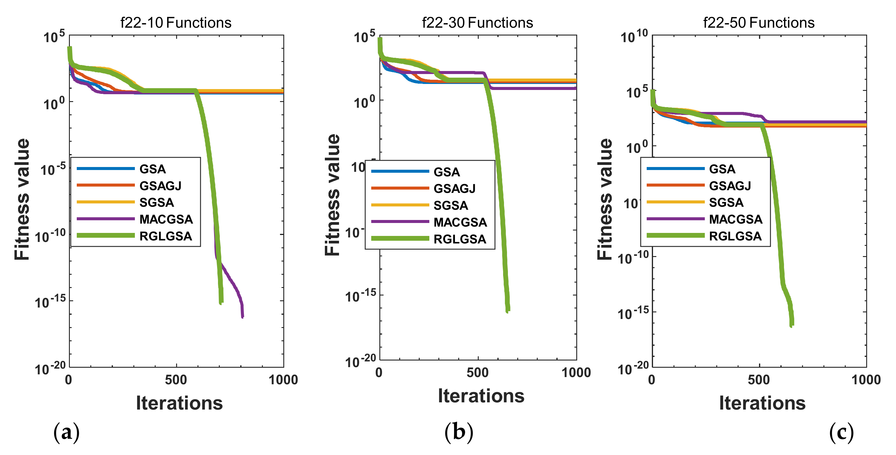
Entropy 24 01826 g006
Figure 7. Convergence curves of function f22: (a) 10 dimensions, (b) 30 dimensions, and (c) 50 dimensions.
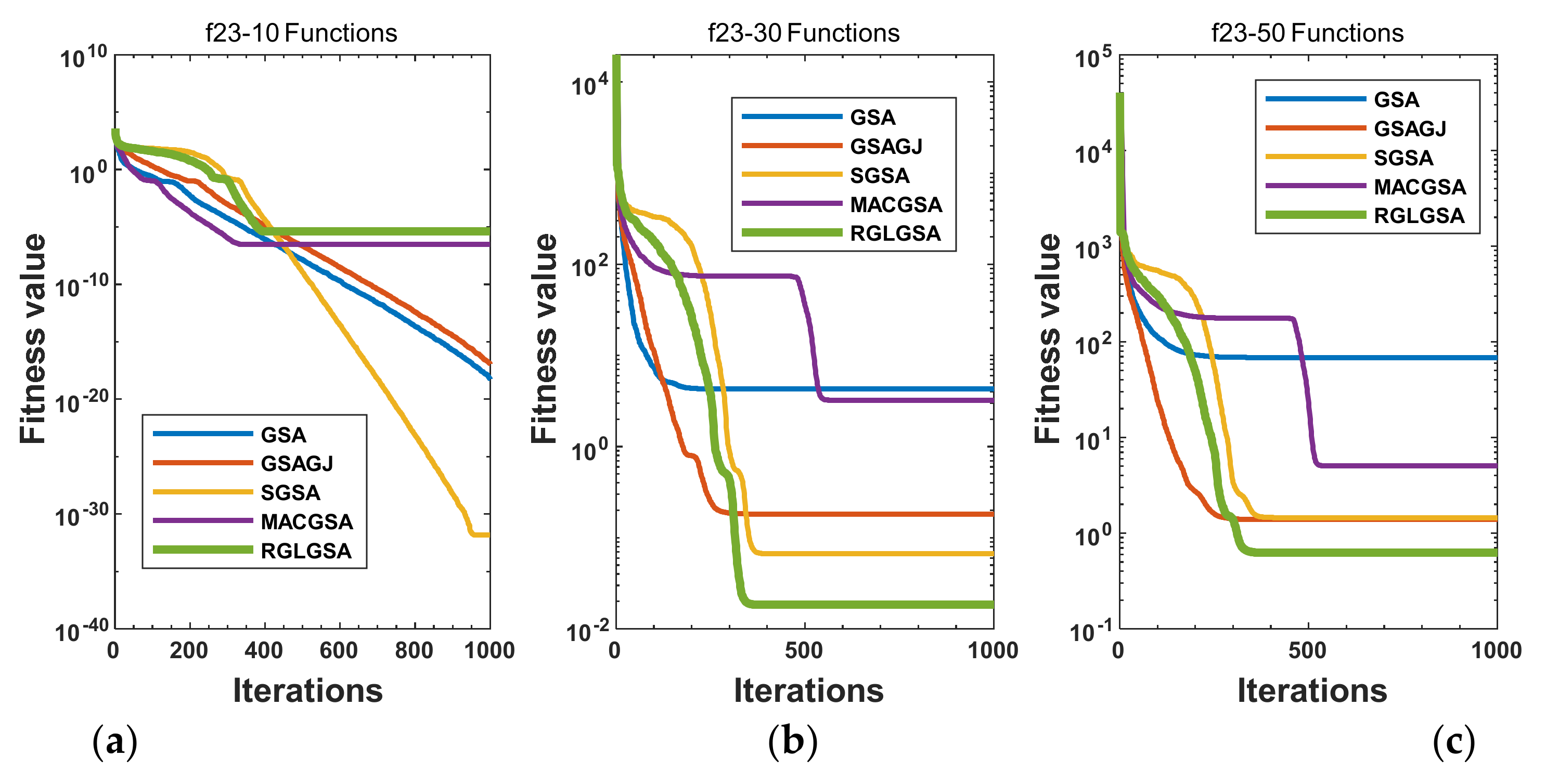
Entropy 24 01826 g007
Figure 8. Convergence curves of function f23: (a) 10 dimensions, (b) 30 dimensions, and (c) 50 dimensions.
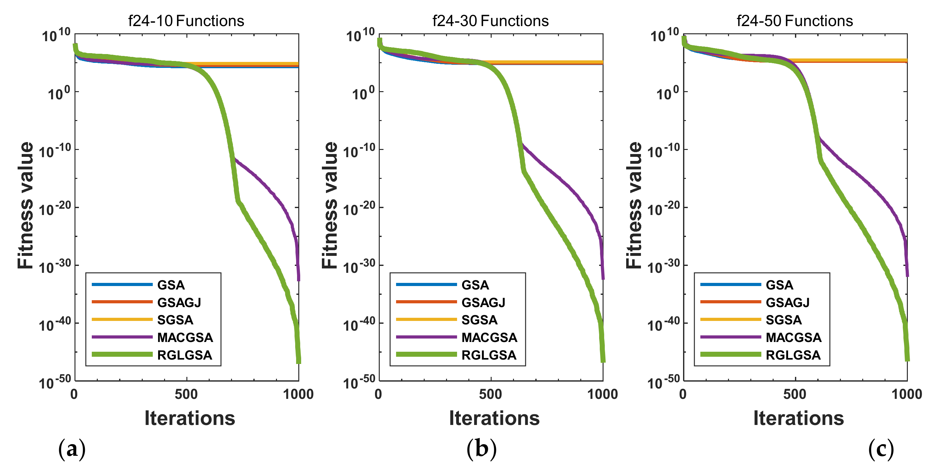
Entropy 24 01826 g008
Figure 9. Convergence curves of function f24: (a) 10 dimensions, (b) 30 dimensions, and (c) 50 dimensions.
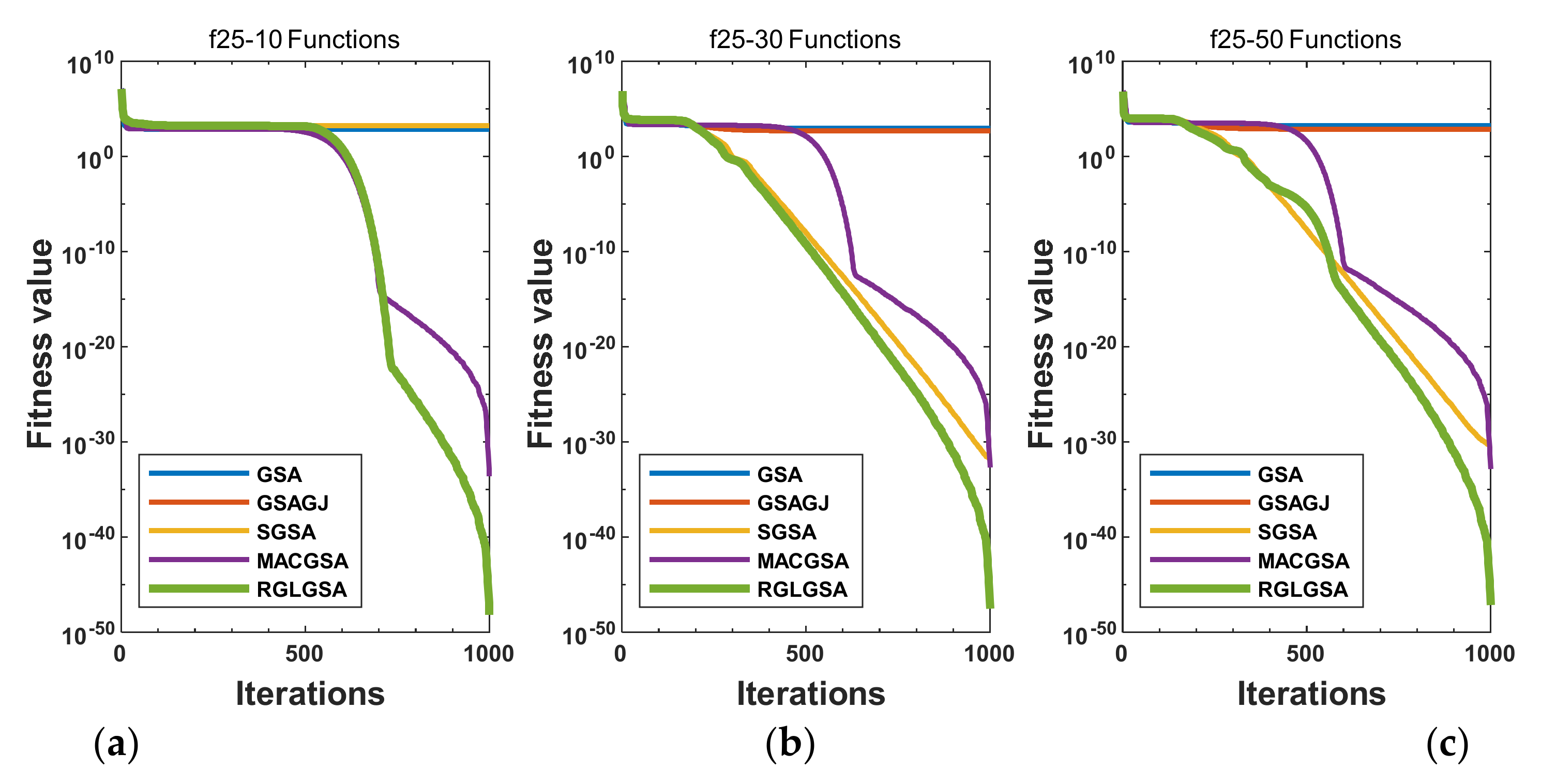
Entropy 24 01826 g009
Figure 10. Convergence curves of function f25: (a) 10 dimensions, (b) 30 dimensions, and (c) 50 dimensions.
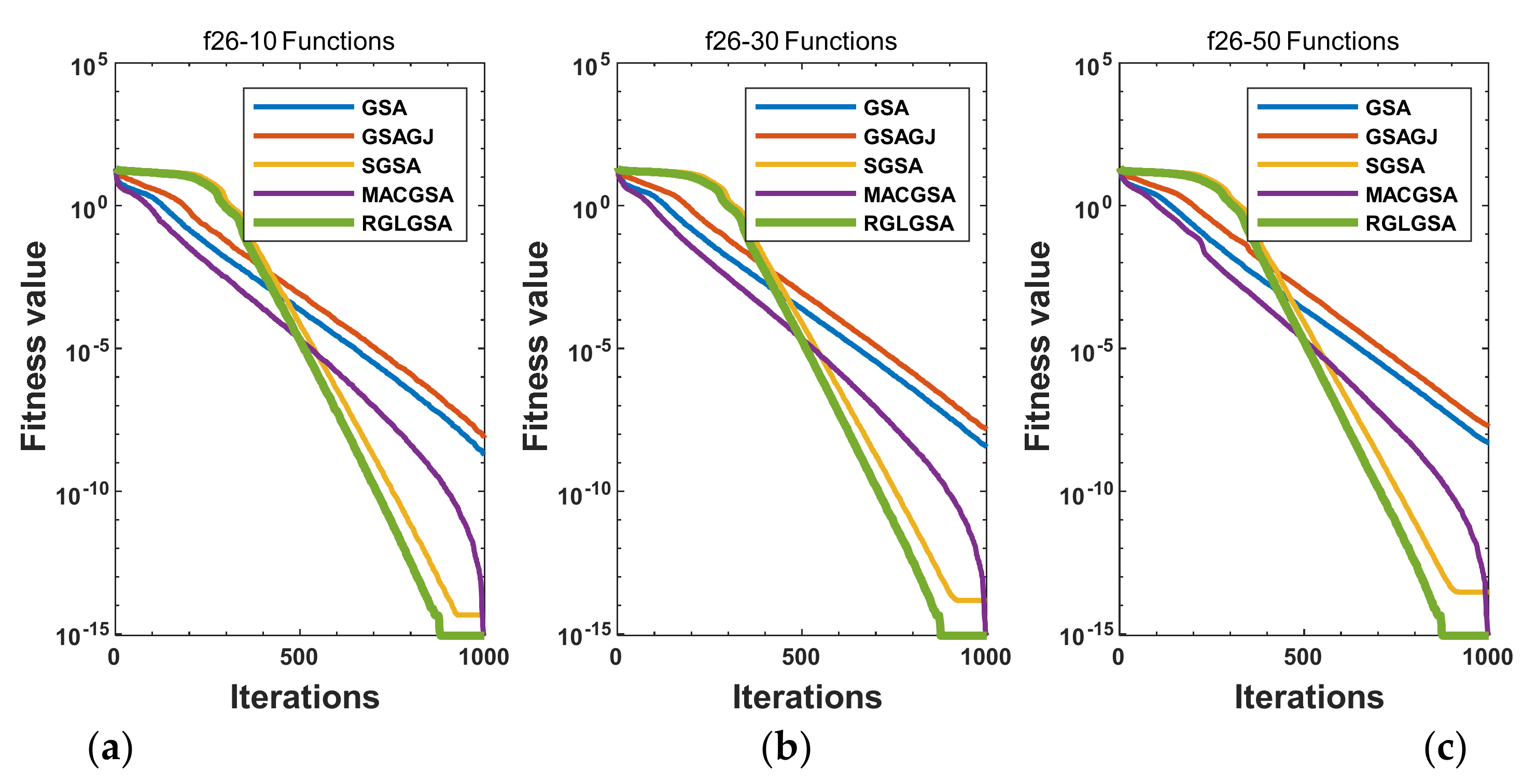
Entropy 24 01826 g010
Figure 11. Convergence curves of function f26: (a) 10 dimensions, (b) 30 dimensions, and (c) 50 dimensions.
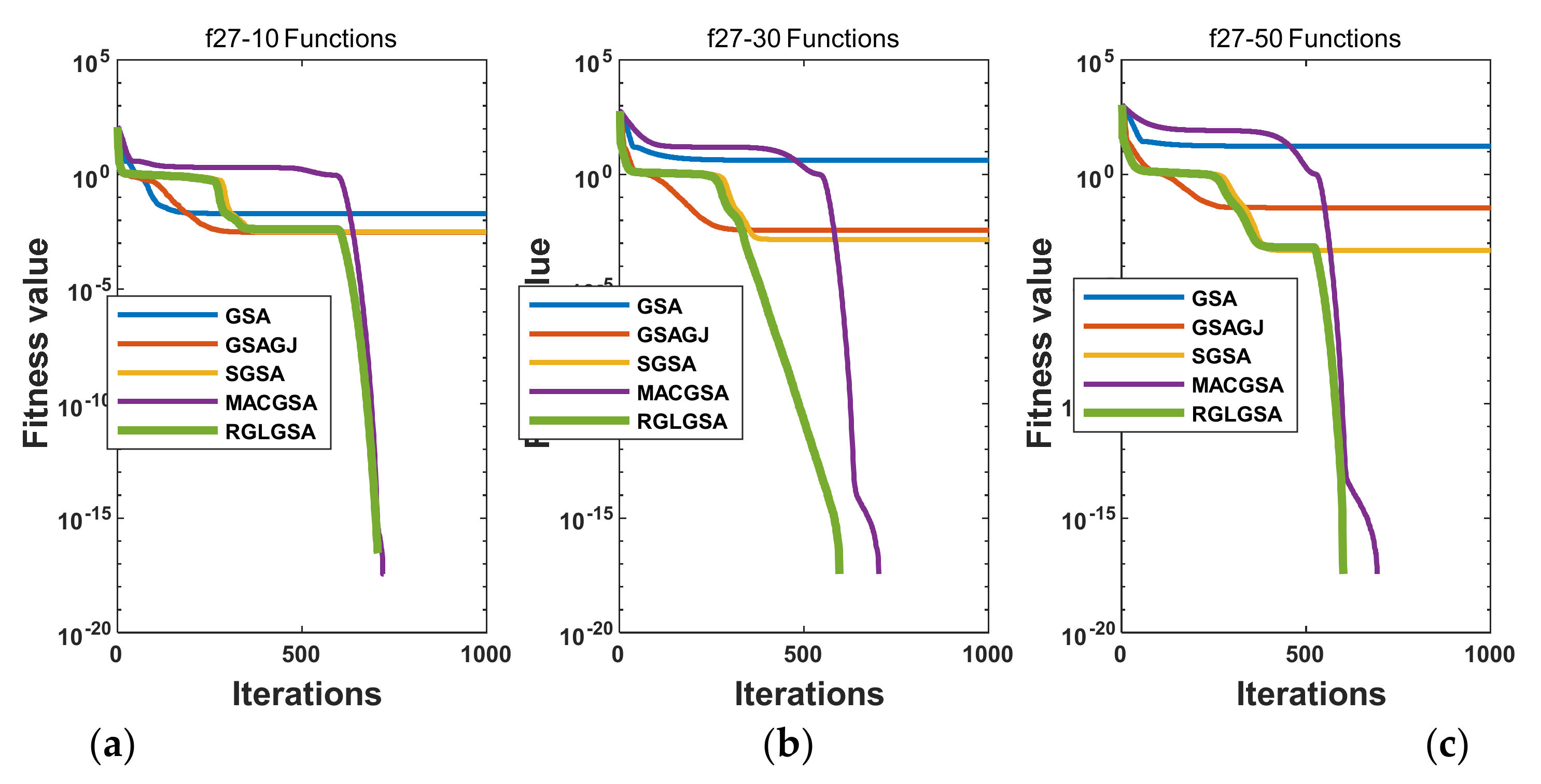
Entropy 24 01826 g011
Figure 12. Convergence curves of function f27: (a) 10 dimensions, (b) 30 dimensions, and (c) 50 dimensions.
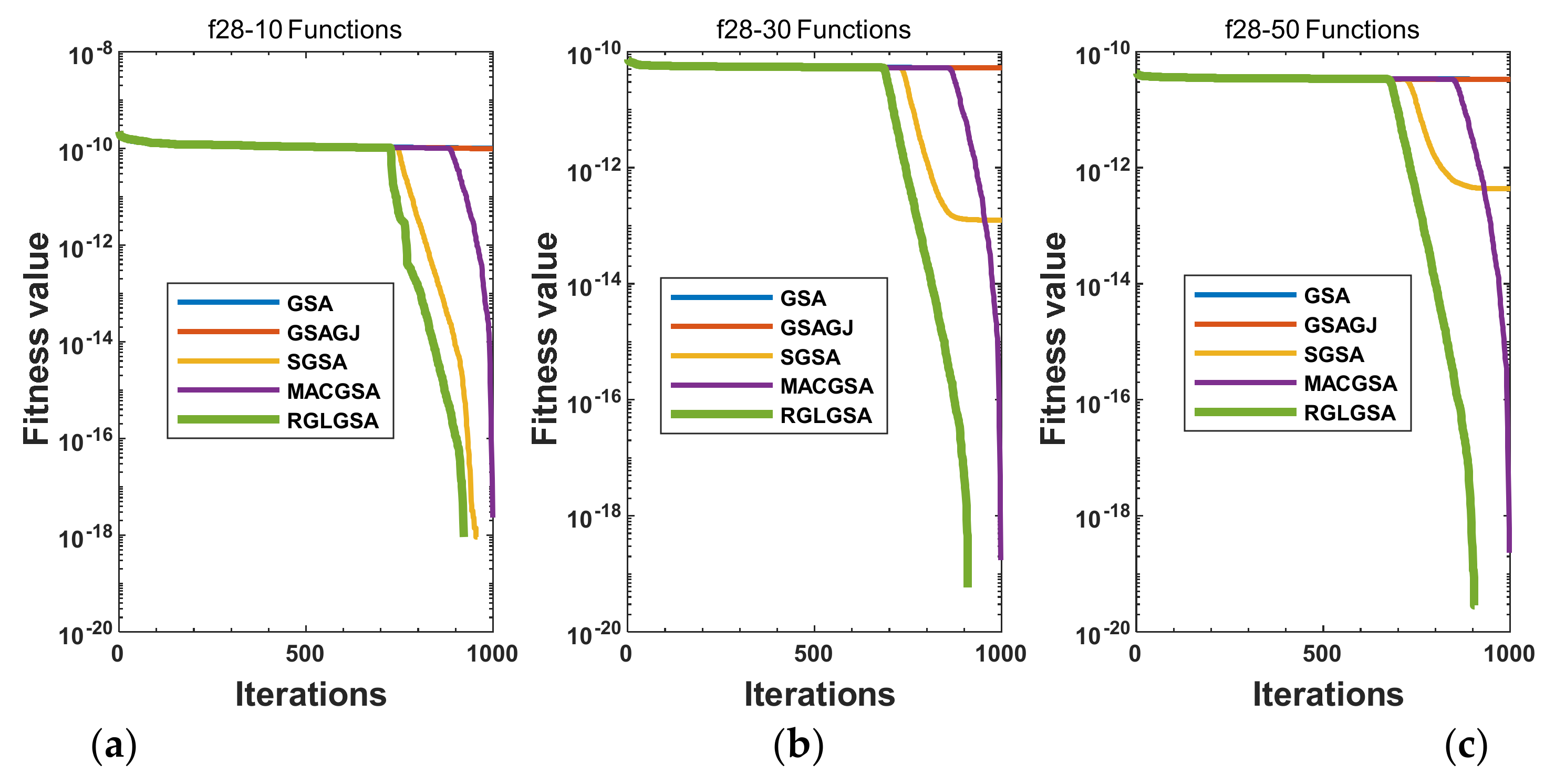
Entropy 24 01826 g012
Figure 13. Convergence curves of function f28: (a) 10 dimensions, (b) 30 dimensions, and (c) 50 dimensions.
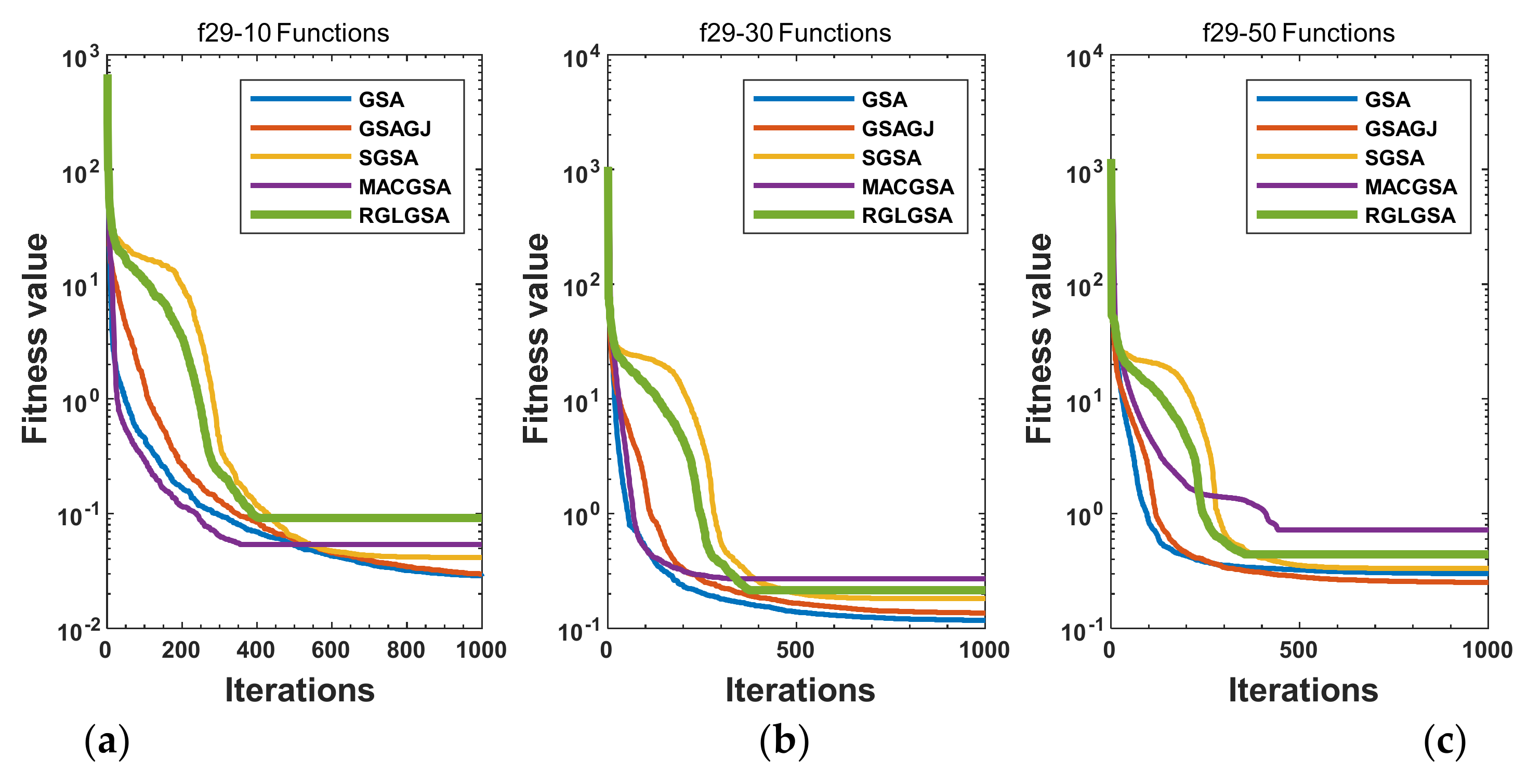
Entropy 24 01826 g013
Figure 14. Convergence curves of function f29: (a) 10 dimensions, (b) 30 dimensions, and (c) 50 dimensions.
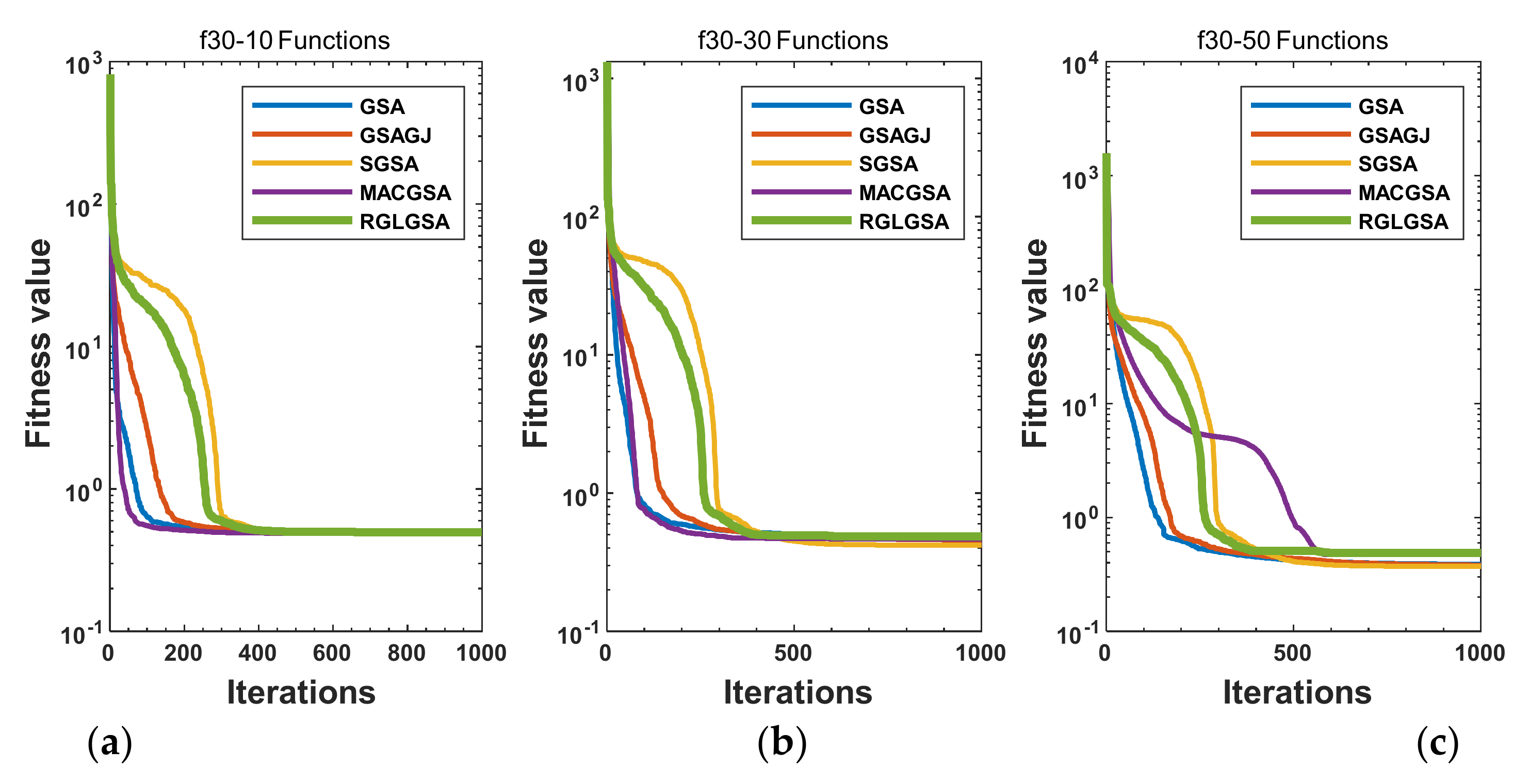
Entropy 24 01826 g014
Figure 15. Convergence curves of function f30: (a) 10 dimensions, (b) 30 dimensions, and (c) 50 dimensions.
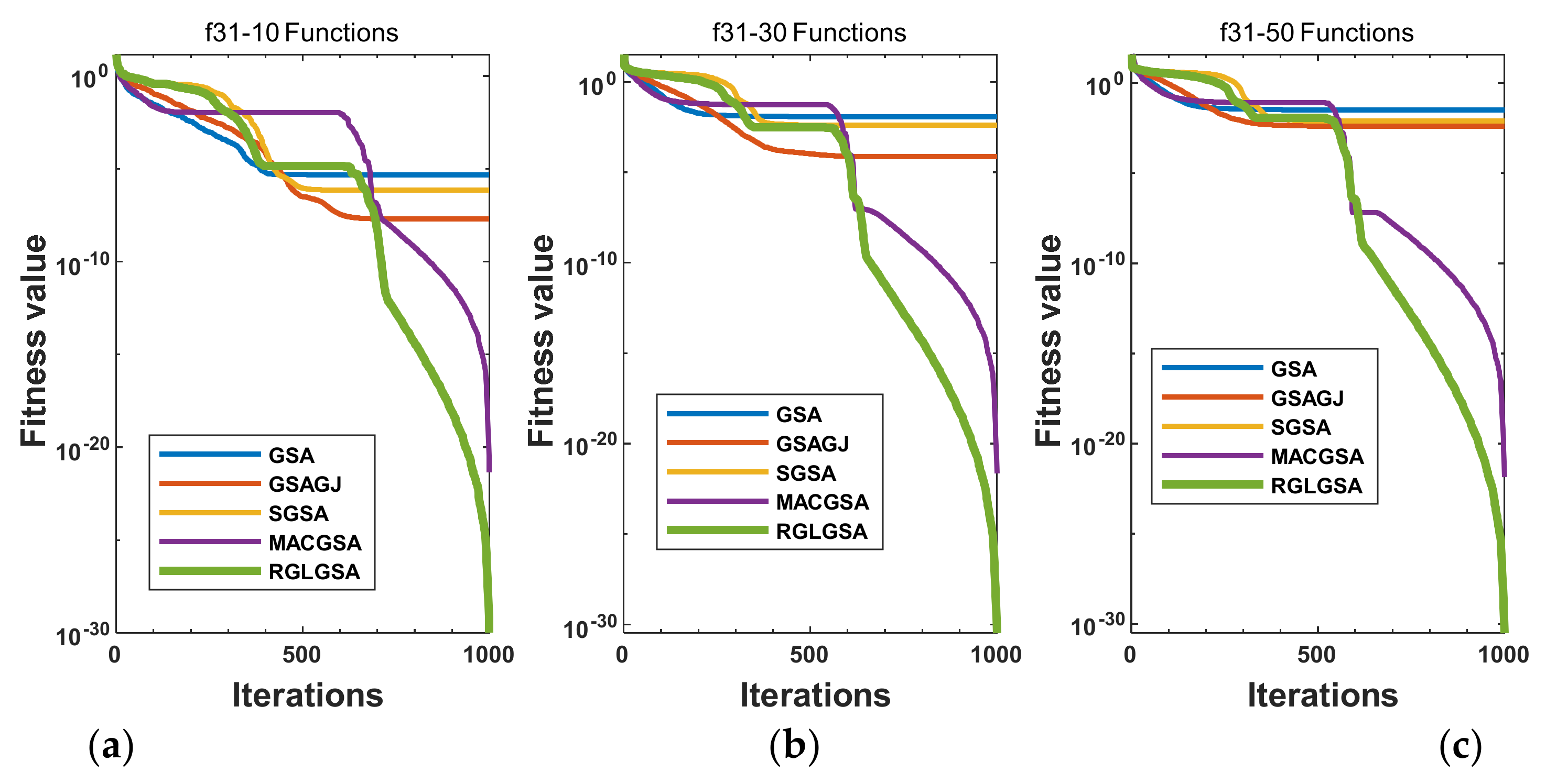
Entropy 24 01826 g015
Figure 16. Convergence curves of function f31: (a) 10 dimensions, (b) 30 dimensions, and (c) 50 dimensions.
Entropy 24 01826 g016
Table 1. Test function set.
Function No.Test FunctionValue Range
1 f 1 ( x ) = i = 1 n x i 2 x i [ 100 , 100 ]
2 f 2 ( x ) = i = 1 n x i + i = 1 n x i x i [ 10 , 10 ]
f 3 ( x ) = max x i x i [ 100 , 100 ]
4 f 4 ( x ) = 20 exp [ 0.2 1 n i = 1 n x i 2 ] exp ( 1 n i = 1 n cos ( 2 π x i ) ) + 20 + e x i [ 32 , 32 ]
5 f 5 ( x ) = i = 1 n x i sin ( x i ) + 0.1 x i x i [ 10 , 10 ]
6 f 6 ( x ) = ( x 2 5.1 4 π x 1 2 - 5 π x 1 6 ) 2 + 10 × ( 1 1 8 π ) cos x 1 + 10 x i [ 10 , 10 ]
7 f 7 ( x ) = i = 1 n ( j = 1 i x j ) 2 x i [ 100 , 100 ]
8 f 8 ( x ) = i = 1 n i x i 4 + r a n d o m 0 , 1 x i [ 1.28 , 1.28 ]
9 f 9 ( x ) = 1 4000 i = 1 n x i 2 i = 1 n cos ( x i i ) + 1 x i [ 600 , 600 ]
10 f 10 ( x ) = i = 1 n x i 2 + ( i = 1 n i 2 x i ) 2 + ( i = 1 n i 2 x i ) 4 x i [ 32 , 32 ]
11 f 11 ( x ) = x 2 + y 2 + 25 ( sin 2 x + sin 2 y ) x i [ 5.14 , 5.14 ]
12 f 12 ( x ) = i = 1 n x i 2 10 cos ( 2 π x i ) + 10 x i [ 5 , 5 ]
13 f 13 ( x ) = i = 1 n ( x i + 0.5 ) 2 x i [ 100 , 100 ]
14 f 14 ( x ) = cos ( 2 π i = 1 n x i 2 ) + 0.1 ( i = 1 n x i 2 ) + 1 x i [ 100 , 100 ]
15 f 15 ( x ) = 0.5 + ( sin x 2 2 + x 1 2 ) 2 0.5 ( 1 + 0.001 ( x 2 2 + x 1 2 ) ) 2 x i [ 10 , 10 ]
Table 2. Test results for f1(x).
DAlgorithmWorstBestMeanSD
30GSA3.1784 × 10−171.1678 × 10−172.0655 × 10−174.9762 × 10⁻¹⁸
RGSA5.7262 × 10−334.1402 × 10−341.0540 × 10−331.0033 × 10⁻³³
GGSA7.8267 × 10−201.6952 × 10−204.2861 × 10−201.5505 × 10⁻²⁰
LGSA1.1171 × 10−277.0551 × 10−311.0968 × 10−282.3663 × 10⁻²⁸
RGGSA2.4777 × 10−382.4197 × 10−398.1763 × 10−394.6307 × 10−39
RLGSA4.3833 × 10−484.9380 × 10−513.9451 × 10−499.0845 × 10−49
GLGSA2.2316 × 10−292.3715 × 10−349.0465 × 10−314.0589 × 10⁻³⁰
RGLGSA1.1227 × 10−531.3115 × 10−561.8360 × 10−543.3730 × 10−54
50GSA1.0370 × 10−164.2637 × 10−177.1477 × 10−171.8306 × 10⁻¹⁷
RGSA7.9678 × 10−324.0968 × 10−331.7587 × 10−321.6047 × 10⁻³²
GGSA3.1420 × 10−197.4754 × 10−202.0370 × 10−196.3958 × 10⁻²⁰
LGSA7.8808 × 10−284.8414 × 10−318.3115 × 10−291.5517 × 10⁻²⁸
RGGSA1.2945 × 10−351.7729 × 10−371.5203 × 10−362.7454 × 10−36
RLGSA3.2260 × 10−481.9879 × 10−506.0257 × 10−497.9558 × 10−49
GLGSA2.6738 × 10−302.0636 × 10−332.3400 × 10−315.0105 × 10⁻³¹
RGLGSA1.4061 × 10−533.6091 × 10−562.1920 × 10−543.3828 × 10−54
Table 3. Test results for f2(x).
DAlgorithmWorstBestMeanSD
30GSA2.9944 × 10−81.8259 × 10−82.3354 × 10−82.8498 × 10⁻⁹
RGSA3.7319 × 10−161.1320 × 10−162.2498 × 10−166.5816 × 10⁻¹⁷
GGSA1.5355 × 10−96.4974 × 10−101.0641 × 10−92.3299 × 10−10
LGSA5.3312 × 10−144.3968 × 10−161.2055 × 10−141.4035 × 10⁻¹⁴
RGGSA1.8821 × 10−173.8605 × 10−191.7182 × 10−183.3370 × 10⁻¹⁸
RLGSA5.1586 × 10−241.0922 × 10−258.5523 × 10−259.6857 × 10⁻²⁵
GLGSA1.6789 × 10−151.0556 × 10−164.5455 × 10−163.1838 × 10⁻¹⁶
RGLGSA4.8916 × 10−272.0799 × 10−281.8049 × 10−271.2726 × 10⁻²⁷
50GSA0.02363.7905 × 10−087.8561 × 10−40.0043
RGSA0.08616.2460 × 10−160.00470.0168
GGSA0.20692.1929 × 10−90.01810.0546
LGSA5.1145 × 10−141.2501 × 10−151.3527 × 10−141.1082 × 10⁻¹⁴
RGGSA0.28332.7805 × 10−130.03200.0748
RLGSA3.1275 × 10−241.8799 × 10−251.2276 × 10−248.5222 × 10⁻²⁵
GLGSA2.8762 × 10−151.3163 × 10−166.1703 × 10−165.8851 × 10⁻¹⁶
RGLGSA8.7338 × 10−271.9445 × 10−282.2760 × 10−271.8606 × 10⁻²⁷
Table 4. Test results for f3(x).
DAlgorithmWorstBestMeanSD
30GSA4.6203 × 10−92.0095 × 10−93.1109 × 10−97.1216 × 10⁻¹⁰
RGSA9.4873 × 10−165.6256 × 10−172.5335 × 10−162.4418 × 10⁻¹⁶
GGSA3.0792 × 10−109.8951 × 10−112.1632 × 10−104.9367 × 10⁻¹¹
LGSA3.2172 × 10−146.3082 × 10−168.1911 × 10−158.6301 × 10⁻¹⁵
RGGSA0.01673.0764 × 10−180.00110.0041
RLGSA4.0438 × 10−242.3297 × 10−267.0978 × 10−258.7193 × 10⁻²⁵
GLGSA2.9153 × 10−154.4903 × 10−175.0494 × 10−166.3364 × 10⁻¹⁶
RGLGSA9.4406 × 10−272.0399 × 10−281.9853 × 10−271.9898 × 10⁻²⁷
50GSA7.30601.49523.89581.2656
RGSA7.74201.41713.80931.6933
GGSA0.00651.8832 × 10−92.4286 × 10−40.0012
LGSA2.9909 × 10−142.6038 × 10−169.7994 × 10−158.8800 × 10⁻¹⁵
RGGSA1.24110.31020.69380.2702
RLGSA6.4042 × 10−241.3099 × 10−251.2454 × 10−241.5236 × 10⁻²⁴
GLGSA5.2383 × 10−152.7606 × 10−177.0144 × 10−161.0081 × 10⁻¹⁵
RGLGSA1.0648 × 10−266.6210 × 10−293.0313 × 10−273.1224 × 10⁻²⁷
Table 5. Test results for f4(x).
DAlgorithmWorstBestMeanSD
30GSA4.5997 × 10−92.5140 × 10−93.5884 × 10−94.2747 × 10⁻¹⁰
RGSA1.5099 × 10−147.9936 × 10−151.0599 × 10−142.7886 × 10⁻¹⁵
GGSA2.5246 × 10−101.2959 × 10−101.6997 × 10−102.7635 × 10⁻¹¹
LGSA9.3259 × 10−148.8818 × 10−161.1428 × 10−141.7165 × 10⁻¹⁴
RGGSA1.5099 × 10−147.9936 × 10−159.6515 × 10−152.5945 × 10⁻¹⁵
RLGSA8.8818 × 10−168.8818 × 10−168.8818 × 10−160
GLGSA4.4409 × 10−158.8818 × 10−161.1250 × 10−159.0135 × 10⁻¹⁶
RGLGSA8.8818 × 10−168.8818 × 10−168.8818 × 10−160
50GSA6.2569 × 10−93.7704 × 10−94.9280 × 10−96.2123 × 10⁻¹⁰
RGSA2.5757 × 10−141.5099 × 10−142.0191 × 10−143.1890 × 10⁻¹⁵
GGSA6.4020 × 10−101.9065 × 10−102.6571 × 10−108.2614 × 10⁻¹¹
LGSA2.2204 × 10−148.8818 × 10−165.7436 × 10−154.4239 × 10⁻¹⁵
RGGSA0.01931.1546 × 10−140.00140.0043
RLGSA8.8818 × 10−168.8818 × 10−168.8818 × 10−160
GLGSA4.4409 × 10−158.8818 × 10−161.2434 × 10−151.0840 × 10⁻¹⁵
RGLGSA8.8818 × 10−168.8818 × 10−168.8818 × 10−160
Table 6. Test results for f5(x).
DAlgorithmWorstBestMeanSD
30GSA2.8447 × 10−91.3648 × 10−92.2171 × 10−93.7633 × 10⁻¹⁰
RGSA0.00453.8202 × 10−188.5381 × 10−40.0013
GGSA1.5427 × 10−107.2127 × 10−111.1032 × 10−101.8751 × 10⁻¹¹
LGSA1.0398 × 10−147.2806 × 10−171.3223 × 10−152.1370 × 10⁻¹⁵
RGGSA0.00694.7484 × 10−210.00140.0021
RLGSA6.9037 × 10−252.8753 × 10−261.2272 × 10−251.3593 × 10⁻²⁵
GLGSA2.3019 × 10−167.6262 × 10−186.1309 × 10−175.3079 × 10⁻¹⁷
RGLGSA2.1912 × 10−273.3527 × 10−292.2977 × 10−284.0053 × 10⁻²⁸
50GSA0.00754.2822 × 10−97.8908 × 10−40.0017
RGSA0.02392.7429 × 10−140.00550.0053
GGSA0.00391.9820 × 10−107.3396 × 10−40.0011
LGSA8.0741 × 10−156.6396 × 10−171.2979 × 10−151.5773 × 10⁻¹⁵
RGGSA0.03611.4921 × 10−50.01050.0086
RLGSA6.5537 × 10−251.5424 × 10−261.4210 × 10−251.2736 × 10⁻²⁵
GLGSA2.4325 × 10−161.1630 × 10−175.7302 × 10−174.5711 × 10⁻¹⁷
RGLGSA9.6359 × 10−286.0262 × 10−293.0080 × 10−282.1554 × 10⁻²⁸
Table 7. Test results for f6(x).
DAlgorithmWorstBestMeanSD
2GSA0.39790.39790.39790
RGSA0.39790.39790.39790
GGSA0.39790.39790.39790
LGSA0.39790.39790.39790
RGGSA0.39790.39790.39790
RLGSA0.39790.39790.39790
GLGSA0.39790.39790.39790
RGLGSA0.39790.39790.39790
Table 8. Test results for f7(x).
DAlgorithmWorstBestMeanSD
30GSA441.6230100.6353232.082873.4886
RGSA3.0106 × 103905.07571.7284 × 103568.6537
GGSA173.783436.2260101.602239.9589
LGSA2.2037 × 10−242.6581 × 10−307.9806 × 10−264.0151 × 10⁻²⁵
RGGSA4.3546 × 103839.77322.3577 × 103895.2346
RLGSA4.2249 × 10−462.3761 × 10−507.2154 × 10−471.1422 × 10−46
GLGSA2.5695 × 10−285.9115 × 10−333.4041 × 10−297.3331 × 10⁻²⁹
RGLGSA1.0902 × 10−518.8591 × 10−552.3283 × 10−523.4958 × 10−52
50GSA1.5986 × 103678.5357988.3067261.3114
RGSA8.8062 × 1033.8307 × 1035.6479 × 1031.2912 × 103
GGSA865.9041351.5170642.5225125.1997
LGSA1.0505 × 10−241.2817 × 10−297.9992 × 10−262.1493 × 10⁻²⁵
RGGSA1.0125 × 1044.1745 × 1036.9878 × 1031.2641 × 103
RLGSA7.9867 × 10−461.2999 × 10−491.1830 × 10−461.8003 × 10−46
GLGSA8.3184 × 10−283.3753 × 10−329.8107 × 10−291.9489 × 10⁻²⁸
RGLGSA3.9046 × 10−519.6762 × 10−565.4271 × 10−528.8234 × 10−52
Table 9. Test results for f8(x).
DAlgorithmWorstBestMeanSD
30GSA0.03860.00900.01930.0072
RGSA0.05870.00930.03010.0118
GGSA0.05470.01670.03100.0105
LGSA1.9174 × 10−48.5337 × 10−84.5438 × 10−54.6017 × 10⁻⁵
RGGSA0.07720.01610.04550.0156
RLGSA1.1234 × 10−47.6825 × 10−73.7319 × 10−53.0182 × 10⁻⁵
GLGSA2.0404 × 10−41.1790 × 10−75.0362 × 10−55.3880 × 10⁻⁵
RGLGSA1.8700 × 10−41.1549 × 10−64.5049 × 10−54.7092 × 10⁻⁵
50GSA0.19320.02960.06270.0317
RGSA0.20040.05170.11210.0359
GGSA0.14530.03070.07830.0290
LGSA2.9610 × 10−43.1457 × 10−65.6102 × 10−55.8344 × 10⁻⁵
RGGSA0.27180.08400.14490.0453
RLGSA1.8462 × 10−46.1063 × 10−73.6584 × 10−53.8892 × 10⁻⁵
GLGSA1.1842 × 10−42.1433 × 10−63.3349 × 10−52.7926 × 10⁻⁵
RGLGSA1.9608 × 10−47.4748 × 10−73.9030 × 10−54.4529 × 10⁻⁵
Table 10. Test results for f9(x).
DAlgorithmWorstBestMeanSD
30GSA7.44111.37464.04201.5575
RGSA0.007402.4653 × 10−40.0014
GGSA0.053700.00790.0162
LGSA0000
RGGSA0.012309.8565 × 10−40.0031
RLGSA0000
GLGSA0000
RGLGSA0000
50GSA23.423711.085017.21323.4714
RGSA0.012400.00150.0036
GGSA1.175900.13190.2313
LGSA0000
RGGSA0.009903.5078 × 10−40.0018
RLGSA0000
GLGSA0000
RGLGSA0000
Table 11. Test results for f10(x).
DAlgorithmWorstBestMeanSD
30GSA22.36929.724715.41512.8357
RGSA30.901710.780420.95845.1313
GGSA20.09706.616012.53343.7834
LGSA7.1106 × 10−247.4616 × 10−301.2373 × 10−241.7594 × 10⁻²⁴
RGGSA45.728323.128035.32096.6800
RLGSA1.0930 × 10−452.7914 × 10−472.5198 × 10−462.5438 × 10−46
GLGSA1.3735 × 10−263.1561 × 10−312.2552 × 10−273.0441 × 10⁻²⁷
RGLGSA2.5063 × 10−517.9170 × 10−536.7030 × 10−526.1941 × 10−52
50GSA49.178618.875031.46716.6325
RGSA47.899627.532037.68315.7390
GGSA42.931514.310229.69478.4815
LGSA2.1156 × 10−239.4851 × 10−294.9534 × 10−245.0170 × 10⁻²⁴
RGGSA83.979655.068267.52948.7154
RLGSA2.2174 × 10−455.9626 × 10−475.5519 × 10−464.4312 × 10−46
GLGSA3.4122 × 10−261.9063 × 10−308.4759 × 10−279.3119 × 10⁻²⁷
RGLGSA6.6221 × 10−511.3981 × 10−521.5619 × 10−511.3807 × 10−51
Table 12. Test results for f11(x).
DAlgorithmWorstBestMeanSD
2GSA6.9837 × 10−192.4931 × 10−211.4808 × 10−191.5281 × 10⁻¹⁹
RGSA1.5693 × 10−363.9431 × 10−393.6757 × 10−374.0331 × 10−37
GGSA1.1021 × 10−213.8066 × 10−242.6538 × 10−222.4632 × 10⁻²²
LGSA2.5328 × 10−251.0902 × 10−352.4752 × 10−266.4866 × 10⁻²⁶
RGGSA1.6362 × 10−414.2936 × 10−442.4011 × 10−423.8616 × 10−42
RLGSA3.1987 × 10−472.1284 × 10−531.9892 × 10−485.9666 × 10−48
GLGSA2.5843 × 10−273.2845 × 10−352.1927 × 10−285.3440 × 10⁻²⁸
RGLGSA4.3268 × 10−536.2023 × 10−605.7435 × 10−541.1301 × 10−53
Table 13. Test results for f12(x).
DAlgorithmWorstBestMeanSD
30GSA21.88917.959714.89123.5586
RGSA34.823513.929422.25395.7095
GGSA26.86399.949618.57264.2961
LGSA0000
RGGSA34.823514.924425.66995.8915
RLGSA0000
GLGSA0000
RGLGSA0000
50GSA50.742922.884133.03266.0459
RGSA50.742923.879037.70897.0031
GGSA47.758021.889137.01256.4396
LGSA0000
RGGSA81.586534.823551.240311.3435
RLGSA0000
GLGSA0000
RGLGSA0000
Table 14. Test results for f13(x).
DAlgorithmWorstBestMeanSD
30GSA0000
RGSA0000
GGSA0000
LGSA0000
RGGSA0000
RLGSA0000
GLGSA0000
RGLGSA0000
50GSA400.63330.9994
RGSA500.66671.2130
GGSA0000
LGSA0000
RGGSA400.76671.0400
RLGSA0000
GLGSA0000
RGLGSA0000
Table 15. Test results for f14(x).
DAlgorithmWorstBestMeanSD
30GSA2.40010.80141.29380.4433
RGSA1.29890.70010.94790.1567
GGSA0.90310.59990.68200.0680
LGSA5.6621 × 10−1501.1361 × 10−151.5394 × 10⁻¹⁵
RGGSA1.40720.80521.12640.1450
RLGSA0000
GLGSA1.1102 × 10−1601.1102 × 10−173.3876 × 10⁻¹⁷
RGLGSA0000
50GSA4.89872.40573.33260.5198
RGSA2.30011.40051.78680.2488
GGSA2.60050.99991.67490.3434
LGSA8.3267 × 10−151.1102 × 10−161.3582 × 10−151.7851 × 10⁻¹⁵
RGGSA2.50081.51831.88900.2373
RLGSA0000
GLGSA2.2204 × 10−1603.3307 × 10−175.9395 × 10⁻¹⁷
RGLGSA0000
Table 16. Test results for f15(x).
DAlgorithmWorstBestMeanSD
2GSA0.00981.3534 × 10−50.00630.0039
RGSA0.00971.0306 × 10−40.00540.0038
GGSA0.00972.7770 × 10−40.00410.0032
LGSA0000
RGGSA0.00975.8631 × 10−40.00570.0033
RLGSA0000
GLGSA0000
RGLGSA0000
Table 17. CEC2017 benchmark function set.
Function No.Test FunctionValue Range
16 f 16 ( x ) = x 1 2 + 10 6 i = 2 n x i 2 x i [ 100 , 100 ]
17 f 17 ( x ) = i = 1 n x i i + 1 x i [ 100 , 100 ]
18 f 18 ( x ) = i = 1 n x i 2 + ( i = 1 n 0.5 x i ) 2 + ( i = 1 n 0.5 x i ) 4 x i [ 100 , 100 ]
19 f 19 ( x ) = i = 1 n 1 ( 100 ( x i 2 x i + 1 ) 2 + ( x i 1 ) 2 ) x i [ 10 , 10 ]
20 f 20 ( x ) = i = 1 n ( x i 2 10 cos ( 2 π x i ) + 10 ) x i [ 5.12 , 5.12 ]
21 g ( x , y ) = 0.5 + ( sin 2 ( x 2 + y 2 ) 0.5 ) ( 1 + 0.001 ( x 2 + y 2 ) ) 2 f 21 ( x ) = g ( x 1 , x 2 ) + g ( x 2 , x 3 ) + ... + g ( x n 1 , x n ) + g ( x n , x 1 ) x i [ 100 , 100 ]
22 y i = x i x i 1 2 r o u n d ( 2 x i ) / 2 x i 1 2 f 22 ( x ) = i = 1 n ( y i 2 10 cos ( 2 π y i ) + 10 ) x i [ 100 , 100 ]
23 y i = 1 + x i 1 4 , i = 1 , ... , n f 23 ( x ) = sin 2 ( π y 1 ) + i = 1 n 1 ( y i 1 ) 2 [ 1 + 10 sin 2 ( π y i + 1 ) ] + ( y n 1 ) 2 [ 1 + sin 2 ( 2 π y n ) ] x i [ 100 , 100 ]
24 f 24 ( x ) = i = 1 n ( 10 6 ) i 1 n 1 x i 2 x i [ 100 , 100 ]
25 f 25 ( x ) = i = 2 n x i 2 + 10 6 x 1 2 x i [ 100 , 100 ]
26 f 26 ( x ) = 20 exp ( 0.2 1 n i = 1 n x i 2 ) exp ( 1 n i = 1 n cos ( 2 π x i ) ) + 20 + e x i [ 32 , 32 ]
27 f 27 ( x ) = 1 4000 i = 1 n x i 2 i = 1 n cos ( x i i ) + 1 x i [ 600 , 600 ]
28 f 28 ( x ) = 10 n 2 i = 1 n ( 1 + i j = 1 32 2 j x i r o u n d ( 2 j x i ) 2 j ) 10 n 1.2 10 n 2 x i [ 100 , 100 ]
29 f 29 ( x ) = i = 1 n x i 2 n 1 / 4 + ( 0.5 i = 1 n x i 2 + i = 1 n x i ) / n + 0.5 x i [ 100 , 100 ]
30 f 30 ( x ) = ( i = 1 n x i 2 ) 2 ( i = 1 n x i ) 2 1 / 2 + ( 0.5 i = 1 n x i 2 + i = 1 n x i ) / n + 0.5 x i [ 100 , 100 ]
31 y i = x i 2 + x i + 1 2 f 31 ( x ) = 1 n 1 i = 1 n 1 ( y i ( sin ( 50 y i 0.2 ) + 1 ) ) 2 2 x i [ 100 , 100 ]
Table 18. Test results for f16(x).
DAlgorithmWorstBestMeanSD
10GSA927.95580.1349131.5188208.5184
GSAGJ2.0404 × 1030.0028416.9901526.4530
SGSA4.5419 × 1030.0048878.36861.1364 × 103
MACGSA2.3696 × 10−291.4460 × 10−342.3722 × 10−305.3549 × 10⁻³⁰
RGLGSA6.4516 × 10−453.8488 × 10−509.3471 × 10−461.8916 × 10−45
30GSA318.60050.001374.132280.4764
GSAGJ906.56671.2895209.9172243.1416
SGSA6.8746 × 1031.09851.5708 × 1031.5861 × 103
MACGSA8.2065 × 10−286.1559 × 10−335.0553 × 10−291.5421 × 10⁻²⁸
RGLGSA2.8601 × 10−424.7112 × 10−481.6732 × 10−435.4578 × 10−43
50GSA355.46760.754681.202686.5312
GSAGJ1.7790 × 1030.0090305.5190394.2691
SGSA5.8571 × 1030.0504988.64991.4382 × 103
MACGSA2.8593 × 10−279.2657 × 10−312.6063 × 10−285.9198 × 10⁻²⁸
RGLGSA1.0848 × 10−422.8539 × 10−471.1947 × 10−432.4321 × 10−43
Table 19. Test results for f17(x).
DAlgorithmWorstBestMeanSD
10GSA8.6678 × 10−111.1821 × 10−141.3260 × 10−112.1751 × 10⁻¹¹
GSAGJ9.4942 × 10−131.0772 × 10−151.7974 × 10−132.7312 × 10⁻¹³
SGSA5.5934 × 10−89.2999 × 10−142.1619 × 10−91.0164 × 10−8
MACGSA2.3449 × 10−791.8483 × 10−931.7312 × 10−805.4499 × 10−80
RGLGSA8.8740 × 10−1084.0256 × 10−1274.6188 × 10−1091.8277 × 10−108
30GSA2.7721 × 10922.83671.1527 × 1085.0804 × 108
GSAGJ6.9577 × 10559.93539.5043 × 1041.9611 × 105
SGSA2.7279 × 108115.36771.4384 × 1075.1481 × 107
MACGSA8.5890 × 10−1021.7331 × 10−1183.1893 × 10−1031.5710 × 10−102
RGLGSA5.9700 × 10−1227.6982 × 10−1352.0933 × 10−1231.0888 × 10−122
50GSA3.4420 × 10291.0669 × 10152.2045 × 10288.1793 × 1028
GSAGJ2.5940 × 10238.6661 × 10101.2069 × 10224.8832 × 1022
SGSA4.1466 × 10248.2921 × 10131.5953 × 10237.6141 × 1023
MACGSA1.7681 × 10−1074.2408 × 10−1216.4581 × 10−1093.2318 × 10−108
RGLGSA1.0401 × 10−1231.5384 × 10−1443.5856 × 10−1251.8973 × 10−124
Table 20. Test results for f18(x).
DAlgorithmWorstBestMeanSD
10GSA3.4437 × 10−183.1320 × 10−192.0191 × 10−187.2080 × 10⁻¹⁹
GSAGJ7.4174 × 10−177.2964 × 10−183.7707 × 10−171.4441 × 10⁻¹⁷
SGSA5.5986 × 10−343.5185 × 10−352.7418 × 10−341.1874 × 10⁻³⁴
MACGSA1.5097 × 10−336.4933 × 10−381.3977 × 10−342.9910 × 10⁻³⁴
RGLGSA4.2237 × 10−481.4052 × 10−515.3557 × 10−499.8273 × 10−49
30GSA22.10131.1135 × 10−170.77734.0327
GSAGJ93.96092.2794 × 10−165.139518.3694
SGSA4.0050 × 103736.03692.3252 × 103872.4120
MACGSA9.4929 × 10−333.0631 × 10−351.8175 × 10−332.6357 × 10⁻³³
RGLGSA2.3447 × 10−473.6562 × 10−503.2662 × 10−485.8753 × 10−48
50GSA812.850456.8831373.8760184.1014
GSAGJ1.3323 × 103134.8774501.4951327.9025
SGSA7.1515 × 1032.8452 × 1034.9205 × 103917.0428
MACGSA1.5722 × 10−325.1156 × 10−361.4101 × 10−333.0031 × 10⁻³³
RGLGSA2.1532 × 10−468.1105 × 10−502.3062 × 10−475.3073 × 10−47
Table 21. Test results for f19(x).
DAlgorithmWorstBestMeanSD
10GSA5.63095.06095.43570.1358
GSAGJ5.70585.03845.39390.1572
SGSA6.63886.01386.38080.1723
MACGSA7.02996.26026.57910.1821
RGLGSA7.46426.48636.91130.2123
30GSA26.607125.560926.07100.2053
GSAGJ26.465925.606526.05220.1975
SGSA28.217126.425626.93330.4014
MACGSA27.876625.872927.15670.3542
RGLGSA27.988227.038127.36090.2197
50GSA49.201645.722146.54390.6840
GSAGJ49.200745.426846.45120.7858
SGSA99.623845.610049.437910.0356
MACGSA48.990946.148747.86390.8066
RGLGSA48.901146.577947.72000.5182
Table 22. Test results for f20(x).
DAlgorithmWorstBestMeanSD
10GSA5.96980.99502.95171.2389
GSAGJ7.959703.68131.8318
SGSA9.94961.98995.57182.0507
MACGSA0000
RGLGSA0000
30GSA23.87907.959714.99073.6105
GSAGJ32.833611.939518.40674.0119
SGSA36.813510.944525.5041 6.6435
MACGSA0000
RGLGSA0000
50GSA42.783220.894131.90506.0093
GSAGJ57.707518.904235.08898.5387
SGSA61.687431.838747.16107.9322
MACGSA0000
RGLGSA0000
Table 23. Test results for f21(x).
DAlgorithmWorstBestMeanSD
10GSA2.73040.93931.58320.4171
GSAGJ3.39761.70652.63640.4612
SGSA3.17661.43502.82820.3456
MACGSA0000
RGLGSA0000
30GSA5.19852.98004.19990.6364
GSAGJ9.77175.31347.68160.9245
SGSA11.93029.295410.89640.6814
MACGSA0000
RGLGSA0000
50GSA8.31524.43916.41130.9250
GSAGJ13.06208.242410.81211.2371
SGSA20.683815.877418.63641.2354
MACGSA0000
RGLGSA0000
Table 24. Test results for f22(x).
DAlgorithmWorstBestMeanSD
10GSA7.344824.46541.5347
GSAGJ825.14761.6727
SGSA11.004036.76142.1870
MACGSA0000
RGLGSA0000
30GSA551222.49598.1175
GSAGJ39 1726.80005.0950
SGSA572035.06678.0982
MACGSA141.008607.767030.2505
RGLGSA0000
50GSA17557108.866729.6133
GSAGJ944259.833312.4957
SGSA1074779.966714.1262
MACGSA850.22390145.2359299.2123
RGLGSA0000
Table 25. Test results for f23(x).
DAlgorithmWorstBestMeanSD
10GSA1.0829 × 10−181.9660 × 10−195.6692 × 10−192.3275 × 10⁻¹⁹
GSAGJ2.7991 × 10−175.0265 × 10−181.1209 × 10−175.3271 × 10⁻¹⁸
SGSA1.4998 × 10−321.4998 × 10−321.4998 × 10−321.1135 × 10−47
MACGSA5.0085 × 10−71.0793 × 10−73.0263 × 10−71.0103 × 10⁻⁷
RGLGSA8.4957 × 10−61.3167 × 10−64.2384 × 10−61.6172 × 10⁻⁶
30GSA45.04205.2599 × 10−184.294710.5661
GSAGJ2.81798.8351 × 10−170.18180.5973
SGSA0.45431.4998 × 10−320.06650.1563
MACGSA3.25952.97523.22150.0676
RGLGSA0.45462.4474 × 10−40.01850.0840
50GSA177.55813.995168.451641.2278
GSAGJ18.09043.6758 × 10−161.39043.4206
SGSA7.72524.1341 × 10−311.45501.7429
MACGSA5.07644.74965.02980.0885
RGLGSA3.28250.00240.62850.8729
Table 26. Test results for f24(x).
DAlgorithmWorstBestMeanSD
10GSA1.5824 × 10565.08452.1881 × 1042.9856 × 104
GSAGJ1.5669 × 1052.2076 × 1033.5142 × 1043.8005 × 104
SGSA2.1238 × 1054.9374 × 1037.4512 × 1045.7663 × 104
MACGSA1.4877 × 10−326.5895 × 10−371.6068 × 10−333.6474 × 10⁻³³
RGLGSA1.2592 × 10−463.9071 × 10−519.0954 × 10−482.6328 × 10−47
30GSA2.2231 × 1051.3209 × 1047.7308 × 1045.3591 × 104
GSAGJ2.4017 × 1059.2003 × 1038.5470 × 1046.0342 × 104
SGSA3.1540 × 1054.3732 × 1041.4493 × 1056.9453 × 104
MACGSA3.6955 × 10−321.8249 × 10−353.2962 × 10−337.3649 × 10⁻³³
RGLGSA1.1867 × 10−466.5780 × 10−501.3542 × 10−472.7548 × 10−47
50GSA2.2231 × 1051.3209 × 1047.7308 × 1045.3591 × 104
GSAGJ2.4017 × 1059.2003 × 1038.5470 × 1046.0342 × 104
SGSA3.1540 × 1054.3732 × 1041.4493 × 1056.9453 × 104
MACGSA3.6955 × 10−321.8249 × 10−353.2962 × 10−337.3649 × 10⁻³³
RGLGSA1.1867 × 10−466.5780 × 10−501.3542 × 10−472.7548 × 10−47
Table 27. Test results for f25(x).
DAlgorithmWorstBestMeanSD
10GSA1.6166 × 103114.4355717.1659407.7005
GSAGJ3.2975 × 103424.61071.6499 × 103749.6641
SGSA3.0122 × 103291.25471.5685 × 103670.7036
MACGSA5.3094 × 10−332.1696 × 10−372.4561 × 10−349.6672 × 10⁻³⁴
RGLGSA7.6013 × 10−481.4909 × 10−516.8777 × 10−491.7501 × 10−48
30GSA2.2537 × 103299.4626872.2012393.5168
GSAGJ2.3856 × 1033.3096 × 10−16486.5437610.2161
SGSA3.2041 × 10−325.0516 × 10−331.3777 × 10−326.3954 × 10⁻³³
MACGSA3.6098 × 10−325.0320 × 10−362.0449 × 10−336.5866 × 10⁻³³
RGLGSA2.1523 × 10−474.3108 × 10−503.0550 × 10−485.7203 × 10−48
50GSA2.8219 × 103566.15101.7062 × 103645.7675
GSAGJ2.6789 × 1031.3496 × 10−15722.0980788.4850
SGSA2.0515 × 10−308.0778 × 10−324.2586 × 10−314.3106 × 10⁻³¹
MACGSA1.3764 × 10−324.2468 × 10−361.3404 × 10−333.3730 × 10⁻³³
RGLGSA6.3641 × 10−471.1221 × 10−496.7762 × 10−481.5149 × 10−47
Table 28. Test results for f26(x).
DAlgorithmWorstBestMeanSD
10GSA2.7037 × 10−91.3481 × 10−91.8639 × 10−93.3343 × 10⁻¹⁰
GSAGJ9.7995 × 10−94.6786 × 10−97.5941 × 10−91.3530 × 10⁻⁹
SGSA7.9936 × 10−154.4409 × 10−154.5593 × 10−156.4863 × 10⁻¹⁶
MACGSA8.8818 × 10−168.8818 × 10−168.8818 × 10−160
RGLGSA8.8818 × 10−168.8818 × 10−168.8818 × 10−160
30GSA4.5600 × 10−92.8379 × 10−93.5839 × 10−94.5843 × 10⁻¹⁰
GSAGJ1.7140 × 10−81.0784 × 10−81.4658 × 10−81.6459 × 10⁻⁹
SGSA2.2204 × 10−147.9936 × 10−151.4744 × 10−143.5343 × 10⁻¹⁵
MACGSA8.8818 × 10−168.8818 × 10−168.8818 × 10−160
RGLGSA8.8818 × 10−168.8818 × 10−168.8818 × 10−160
50GSA8.2910 × 10−93.6928 × 10−94.9393 × 10−98.8854 × 10⁻¹⁰
GSAGJ2.4806 × 10−81.5528 × 10−81.9258 × 10−82.2218 × 10⁻⁹
SGSA5.7732 × 10−141.5099 × 10−142.9073 × 10−147.5758 × 10⁻¹⁵
MACGSA8.8818 × 10−168.8818 × 10−168.8818 × 10−160
RGLGSA8.8818 × 10−168.8818 × 10−168.8818 × 10−160
Table 29. Test results for f27(x).
DAlgorithmWorstBestMeanSD
10GSA0.076200.02000.0205
GSAGJ0.027000.00300.0061
SGSA0.017200.00310.0056
MACGSA0000
RGLGSA0000
30GSA9.52271.77634.21291.7361
GSAGJ0.051500.00380.0108
SGSA0.014800.00150.0040
MACGSA0000
RGLGSA0000
50GSA25.166911.459417.44864.1201
GSAGJ0.176100.03560.0477
SGSA0.014804.9241e-040.0027
MACGSA0000
RGLGSA0000
Table 30. Test results for f28(x).
DAlgorithmWorstBestMeanSD
10GSA1.1961 × 10−106.7969 × 10−111.0001 × 10−101.1193 × 10⁻¹¹
GSAGJ1.2086 × 10−106.9683 × 10−119.8470 × 10−111.2157 × 10⁻¹¹
SGSA0000
MACGSA0000
RGLGSA0000
30GSA5.8032 × 10−114.6224 × 10−115.2202 × 10−113.1700 × 10⁻¹²
GSAGJ5.6719 × 10−114.7120 × 10−115.2218 × 10−112.6389 × 10⁻¹²
SGSA5.8824 × 10−1301.2443 × 10−131.9250 × 10⁻¹³
MACGSA0000
RGLGSA0000
50GSA3.5579 × 10−113.1050 × 10−113.3152 × 10−119.9662 × 10⁻¹³
GSAGJ3.4840 × 10−112.7680 × 10−113.3151 × 10−111.4994 × 10⁻¹²
SGSA1.2293 × 10−128.3267 × 10−154.3324 × 10−133.1526 × 10⁻¹³
MACGSA0000
RGLGSA0000
Table 31. Test results for f29(x).
DAlgorithmWorstBestMeanSD
10GSA0.50500.17700.30010.0798
GSAGJ0.35420.14850.25150.0563
SGSA0.51030.21740.33320.0810
MACGSA1.51000.42780.72520.2975
RGLGSA0.64820.30330.44030.0917
30GSA0.16520.04400.11740.0290
GSAGJ0.19380.08150.13620.0292
SGSA0.27390.11080.18150.0425
MACGSA0.42960.16370.27190.0714
RGLGSA0.30360.12040.21530.0409
50GSA0.50500.17700.30010.0798
GSAGJ0.35420.14850.25150.0563
SGSA0.51030.21740.33320.0810
MACGSA1.51000.42780.72520.2975
RGLGSA0.64820.30330.44030.0917
Table 32. Test results for f30(x).
DAlgorithmWorstBestMeanSD
10GSA0.50080.35700.49250.0267
GSAGJ0.50100.43870.49440.0175
SGSA0.50090.31100.48950.0412
MACGSA0.50000.39650.48600.0285
RGLGSA0.50000.45740.49810.0081
30GSA0.50130.43440.48840.0159
GSAGJ0.50100.32330.45810.0495
SGSA0.50160.27670.42040.0553
MACGSA0.50000.35680.46610.0438
RGLGSA0.50000.41590.48510.0263
50GSA0.61560.24040.38720.0743
GSAGJ0.44950.27430.38140.0405
SGSA0.56870.27300.37260.0542
MACGSA0.50000.34220.47110.0465
RGLGSA0.50000.44510.49000.0154
Table 33. Test results for f31(x).
DAlgorithmWorstBestMeanSD
10GSA1.0420 × 10−42.7999 × 10−344.6894 × 10−61.9938 × 10−5
GSAGJ2.8974 × 10−72.1420 × 10−321.9555 × 10−87.1460 × 10−8
SGSA1.9305 × 10−507.0894 × 10−73.5154 × 10−6
MACGSA1.1429 × 10−215.5902 × 10−244.5938 × 10−223.0559 × 10⁻²²
RGLGSA7.1484 × 10−302.1262 × 10−321.0346 × 10−301.3575 × 10⁻³⁰
30GSA0.07861.5937 × 10−50.01180.0185
GSAGJ5.8248 × 10−41.3017 × 10−107.2445 × 10−51.4989 × 10−4
SGSA0.02611.4485 × 10−60.00400.0063
MACGSA7.9223 × 10+1.4338 × 10−232.2198 × 10−221.9444 × 10⁻²²
RGLGSA1.1549 × 10−309.2467 × 10−333.4346 × 10−312.8391 × 10⁻³¹
50GSA0.07856.1868 × 10−40.01590.0207
GSAGJ0.01891.0070 × 10−50.00310.0050
SGSA0.05485.2674 × 10−40.01010.0146
MACGSA3.8503 × 10−199.9380 × 10−211.2760 × 10−198.0890 × 10⁻²⁰
RGLGSA1.0666 × 10−256.5193 × 10−281.6474 × 10−262.0978 × 10⁻²⁶
Publisher’s Note: MDPI stays neutral with regard to jurisdictional claims in published maps and institutional affiliations.

