
Mean Hitting Time for Random Walks on a Class of Sparse Networks


Abstract
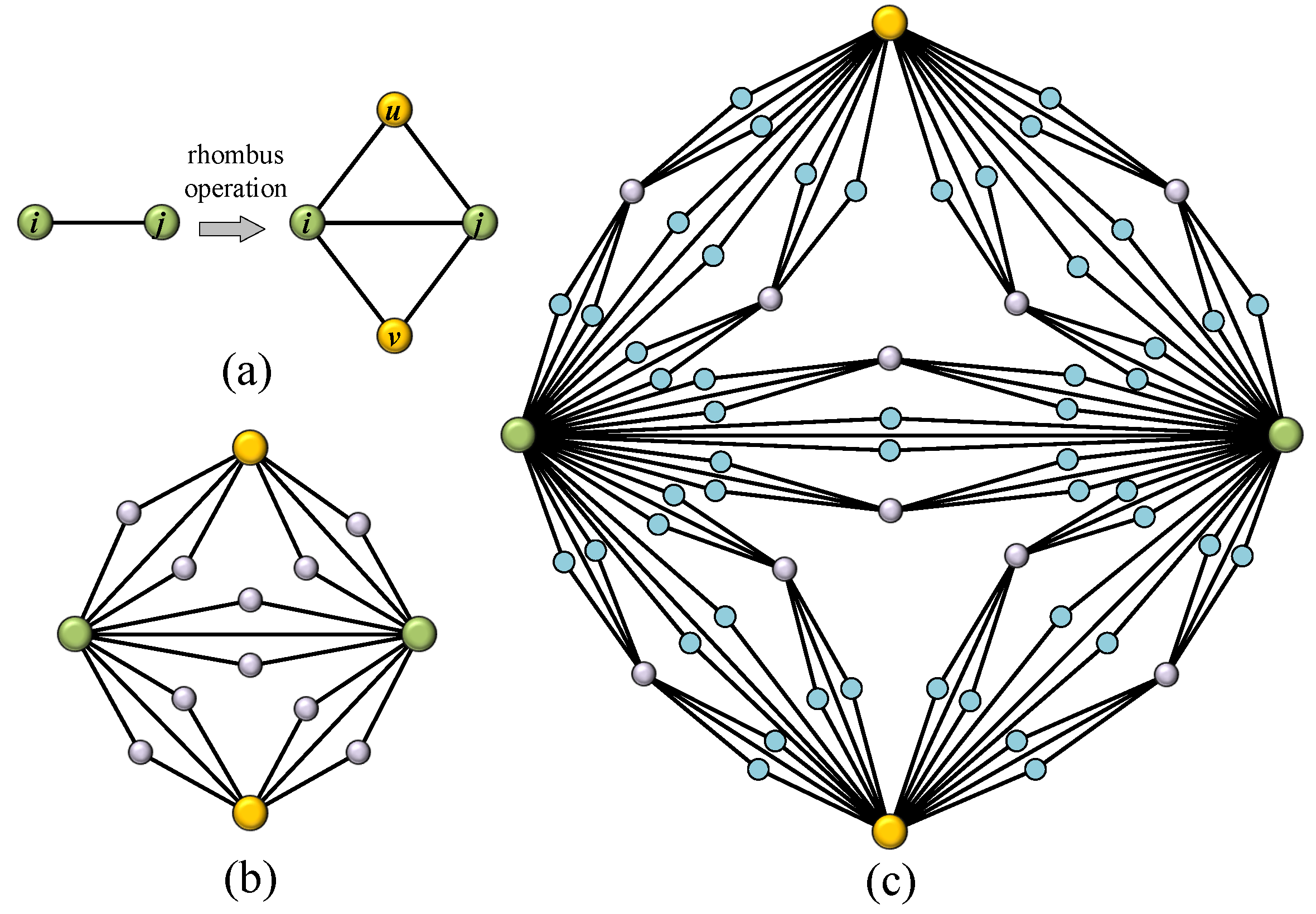
:1. Introduction
2. Topological Characteristics of the Network
2.1. Average Degree
2.2. Cumulative Degree Distribution
2.3. Clustering Coefficient
2.4. Diameter
3. Random Walks and Electrical Networks
3.1. Related Matrices
3.2. Effective Resistances
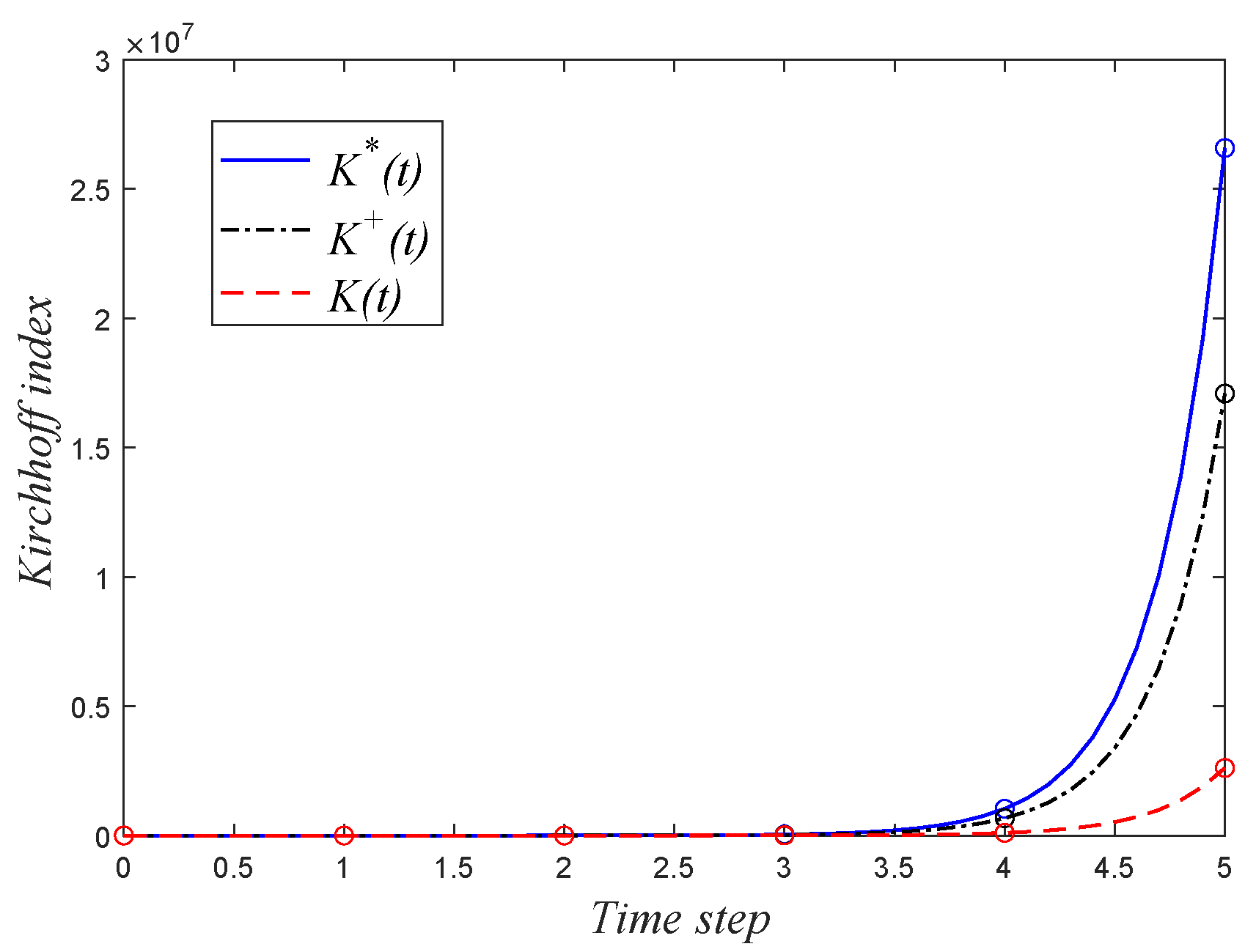
4. Mean Hitting Time
5. Conclusions
Author Contributions
Funding
Data Availability Statement
Conflicts of Interest
Appendix A. The Proof of Lemma 6
Appendix B. The Proof of Lemma 8
References
- Newman, M.E.J. Networks: An Introduction; Oxford University Press: New York, NY, USA, 2010. [Google Scholar]
- An, Z.; Merrill, N.J.; Mcquade, S.T.; Piccoli, B. Equilibria and control of metabolic networks with enhancers and inhibitors. Math. Eng. 2019, 1, 648–671. [Google Scholar] [CrossRef]
- Pan, W.F.; Ming, H.; Chai, C.L. Structure, Dynamics, and Applications of Complex Networks in Software Engineering. Math. Probl. Eng. 2021, 2021, 6734248. [Google Scholar] [CrossRef]
- Hatton, I.A.; McCann, K.S.; Fryxell, J.M.; Davies, T.J.; Smerlak, M.; Sinclair, A.R.E.; Loreau, M. The predator-prey power law: Biomass scaling across terrestrial and aquatic biomes. Science 2015, 349, aac6284. [Google Scholar] [CrossRef]
- Kirkland, S. Fastest expected time to mixing for a Markov chain on a directed graph. Linear Algebra Its Appl. 2010, 433, 1988–1996. [Google Scholar] [CrossRef] [Green Version]
- Levene, M.; Loizou, G. Kemeny’s constant and the random surfer. Am. Math. Mon. 2002, 109, 741–745. [Google Scholar] [CrossRef] [Green Version]
- Zhang, Z.Z.; Sheng, Y.B.; Hu, Z.Y.; Chen, G.R. Optimal and suboptimal networks for efficient navigation measured by mean-first passage time of random walks. Chaos 2012, 22, 043129. [Google Scholar] [CrossRef] [PubMed] [Green Version]
- Wei, W.Y.; Chen, H. Salient object detection based on weighted hypergraph and random walk. Math. Probl. Eng. 2020, 2020, 2073140. [Google Scholar] [CrossRef]
- Chelali, M.; Kurtz, C.; Puissant, A.; Vincent, N. From pixels to random walk based segments for image time series deep classification. In International Conference on Pattern Recognition and Artificial Intelligence; Springer: Cham, Switzerland, 2020. [Google Scholar]
- Baum, D.; Weaver, J.C.; Zlotnikov, I.; Knötel, D.; Tomholt, L.; Dean, M.N. High-throughput segmentation of tiled biological structures using random salk distance transforms. Integr. Comp. Biol. 2019, 6, 6. [Google Scholar]
- Dhahri, A.; Mukhamedov, F. Open quantum random walks and quantum markov chains. Funct. Anal. Its Appl. 2019, 53, 137–142. [Google Scholar] [CrossRef]
- Zhang, K.; Gui, H.; Luo, Z.; Li, D. Matching for navigation map building for automated guided robot based on laser navigation without a reflector. Ind. Robot 2019, 46, 17–30. [Google Scholar] [CrossRef]
- Li, L.; Sun, W.G.; Wang, G.X.; Xu, G. Mean first-passage time on a family of small-world treelike networks. Int. J. Mod. Phys. C 2014, 25, 1350097. [Google Scholar] [CrossRef]
- Dai, M.F.; Sun, Y.Q.; Sun, Y.; Xi, L.; Shao, S. The entire mean weighted first-passage time on a family of weighted treelike networks. Sci. Rep. 2016, 6, 28733. [Google Scholar] [CrossRef] [Green Version]
- Zhang, Z.Z.; Lin, Y.; Ma, Y.J. Effect of trap position on the efficiency of trapping in treelike scale-free networks. J. Phys. A Math. Theor. 2011, 44, 075102. [Google Scholar] [CrossRef]
- Dai, M.F.; Yue, Z.; He, J.J.; Wang, X.; Sun, Y.; Su, W. Two types of weight-dependent walks with a trap in weighted scale-free treelike networks. Sci. Rep. 2018, 8, 1544. [Google Scholar] [CrossRef] [PubMed] [Green Version]
- Wang, X.M.; Ma, F. Constructions and properties of a class of random scale-free networks. Chaos 2020, 30, 043120. [Google Scholar] [CrossRef] [PubMed]
- Sheng, Y.B.; Zhang, Z.Z. Low-Mean Hitting Time for Random Walks on Heterogeneous Networks. IEEE Trans. Inf. Theory 2019, 65, 6898–6910. [Google Scholar] [CrossRef]
- Del Genio, C.I.; Gross, T.; Bassler, K.E. All scale-free network are sparse. Phys. Rev. Lett. 2011, 107, 178701. [Google Scholar] [CrossRef] [Green Version]
- Foster, R.M. The average impedance of an electrical network. Contrib. Appl. Mech. (Reissner Anniv. Vol.) 1949, 333–340. [Google Scholar]
- Chen, H.Y. Random walks and the effective resistance sum rules. Discret. Appl. Math. 2010, 158, 1691–1700. [Google Scholar] [CrossRef] [Green Version]
- Klein, D.J.; Randić, M. Resistance distance. J. Math. Chem. 1993, 1, 81–95. [Google Scholar] [CrossRef]
- Chen, H.Y.; Zhang, F.J. Resistance distance and the normalized Laplacian spectrum. Discret. Appl. Math. 2007, 155, 654–661. [Google Scholar] [CrossRef] [Green Version]
- Gutman, I.; Mohar, B. The quasi-Wiener and the Kirchhoff indices coincide. J. Chem. Inf. Model. 1996, 36, 982–985. [Google Scholar] [CrossRef]
- Kemeny, J.G.; Snell, J.L. Finite Markov Chains; Springer: New York, NY, USA, 1976. [Google Scholar]
- Condamin, S.; Benichou, O.; Tejedor, V.; Voituriez, R.; Klafter, J. First-passage times in complex scale-invariant media. Nature 2007, 450, 77–80. [Google Scholar] [CrossRef] [PubMed] [Green Version]
- Tian, Y. Reverse order laws for the generalized inverses of multiple matrix products. Linear Algebra Its Appl. 1944, 211, 85–100. [Google Scholar] [CrossRef] [Green Version]
- Bapat, R.B. Resistance distance in graphs. Mathmatics Stud. 1999, 68, 87–98. [Google Scholar]

| t | k | ||
|---|---|---|---|
| 0 | 2 | ||
| 1 | |||
| 2 | |||
| ⋯ | ⋯ | ⋯ | ⋯ |
| ⋯ | ⋯ | ⋯ | ⋯ |
| t |
Publisher’s Note: MDPI stays neutral with regard to jurisdictional claims in published maps and institutional affiliations. |
© 2021 by the authors. Licensee MDPI, Basel, Switzerland. This article is an open access article distributed under the terms and conditions of the Creative Commons Attribution (CC BY) license (https://creativecommons.org/licenses/by/4.0/).
Share and Cite
Su, J.; Wang, X.; Yao, B. Mean Hitting Time for Random Walks on a Class of Sparse Networks. Entropy 2022, 24, 34. https://doi.org/10.3390/e24010034
Su J, Wang X, Yao B. Mean Hitting Time for Random Walks on a Class of Sparse Networks. Entropy. 2022; 24(1):34. https://doi.org/10.3390/e24010034
Chicago/Turabian StyleSu, Jing, Xiaomin Wang, and Bing Yao. 2022. "Mean Hitting Time for Random Walks on a Class of Sparse Networks" Entropy 24, no. 1: 34. https://doi.org/10.3390/e24010034
APA StyleSu, J., Wang, X., & Yao, B. (2022). Mean Hitting Time for Random Walks on a Class of Sparse Networks. Entropy, 24(1), 34. https://doi.org/10.3390/e24010034