3.1. General Properties
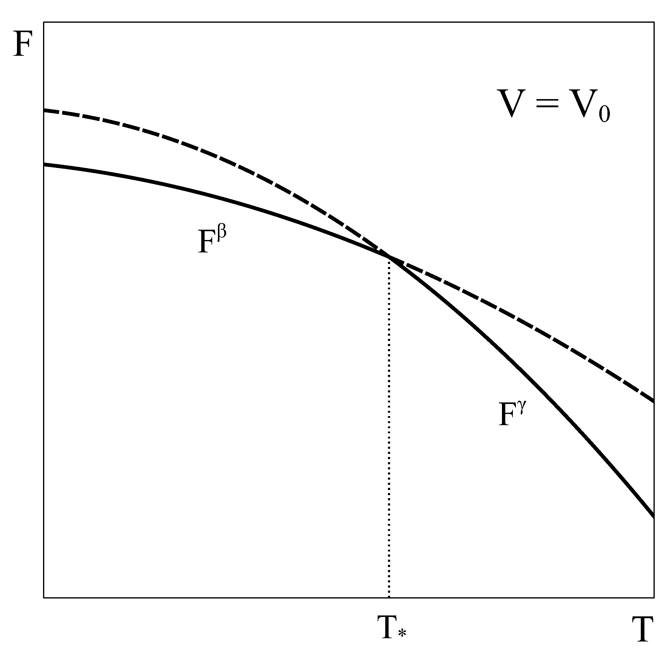
Let us now consider an approach similar to the previous one, but applied to a constant volume transition. As the equilibrium of the system under constant
T and
V is given by the minimum of the Helmholtz potential, let us schematically represent typical Helmholtz curves of phases
and
as a function of temperature under constant
conditions (
Figure 2).
By following a similar reasoning to that of
Section 2, it could be concluded that phase
is the stable phase below temperature
and phase
is the stable one above it. Additionally, it could be thought that at
, both phases could coexist in equilibrium. However, this argument has two flaws. First, nothing ensures that at volume
and
the pressure of phase
given by its equation of state matches that of phase
. In fact, in general, this condition is not met. Therefore, the equality of all the characteristic intensive variables of each phase, a necessary requirement for the equilibrium of two phases, would not be satisfied [
4,
5]. Secondly, nothing ensures that there is no other Helmholtz energy curve that fulfills the constant volume condition and also lies below both single-phase Helmholtz energy curves, so giving the actual minimum. This could be achieved, for example, by combining different amounts of phases
and
at each temperature, thanks to the fact that volume is an extensive quantity. In fact, in the following we will see that such a curve indeed exists!
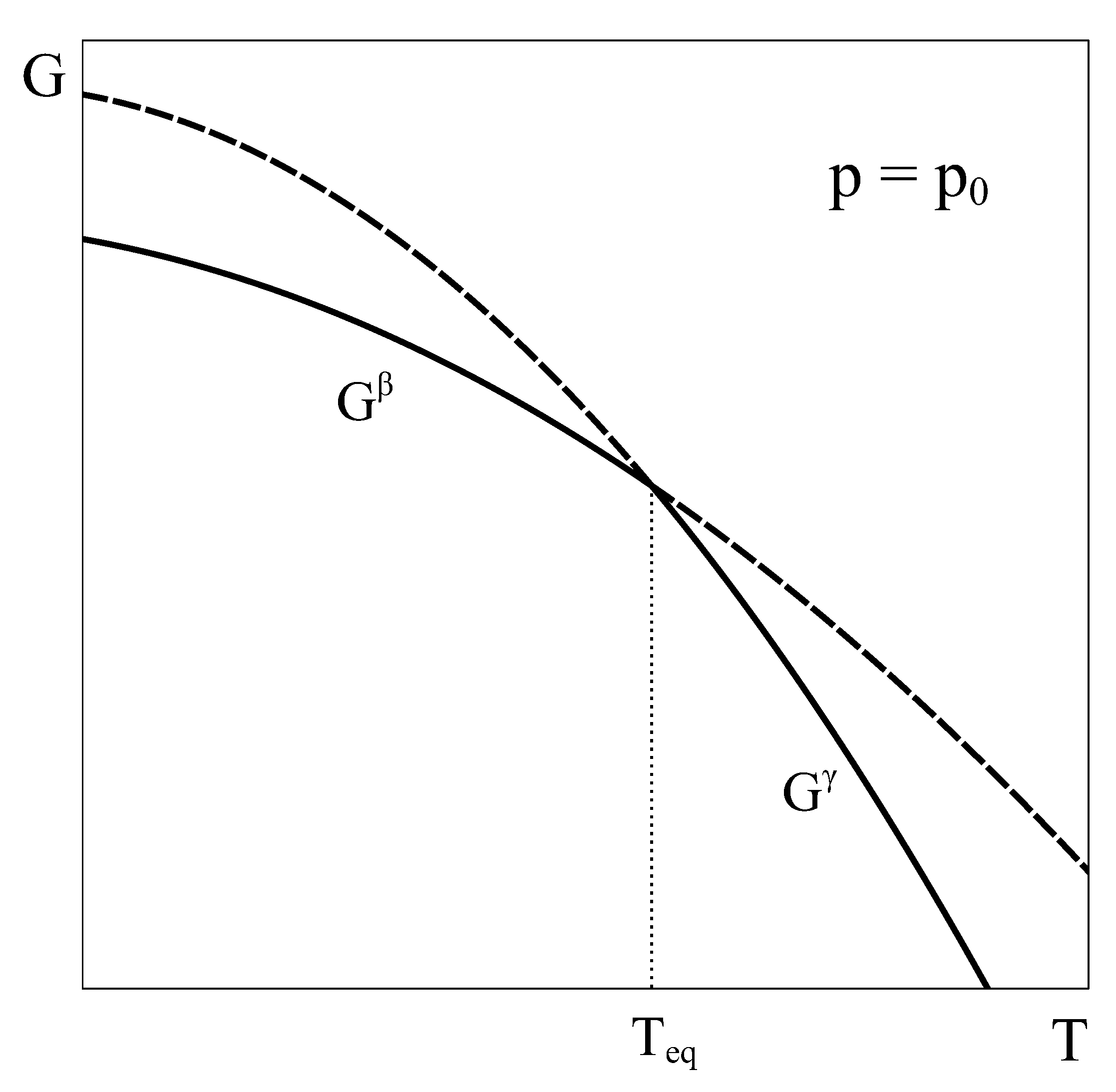
This analogy highlights other aspects of the key role played by the Gibbs energy. First, by exclusively depending on the intensive variables p and T, it can be assured that when two Gibbs energy curves at constant p intersect at an equilibrium temperature (or two curves at constant T intersect at an equilibrium pressure) the other intensive variable also coincides, ensuring equilibrium. Secondly, the absence of natural extensive variables of G precludes the possibility of combining two single phase Gibbs energy curves into a new curve that could lie below both single-phase characteristic G curves.
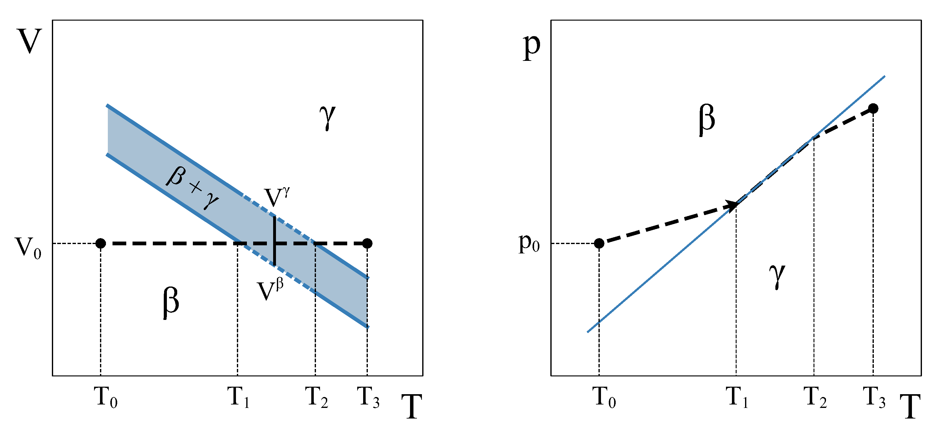
Therefore, how can a constant volume phase transformation be analyzed? The first thing to notice is that a constant volume first-order transformation must occur over a temperature range. To see this, let us go back to our simple system analyzed in
Section 2. A
phase diagram for this system (
Figure 3, left panel) shows two single-phase regions and an area in the
plane where
and
phases coexist. The existence of an area instead of a line is a consequence of the finite jump in volume at each temperature associated with the first order PT. If we want the system now to transform from phase
to phase
at a constant volume
, the temperature during the phase transformation must necessarily change. By starting in the
single-phase field at
and warming up the system at constant volume,
will start nucleating at
, but the phase transformation will not end until temperature
is reached (
Figure 3). During the coexistence, both phases must be at equilibrium. This condition requires the equality of temperature, pressure, and chemical potential [
4,
5]. These conditions are met if the system evolves along the
coexistence line in the
phase diagram (
Figure 3, right panel). Therefore, during phase coexistence at constant volume,
p and
T change and are linked by the coexistence line. As the volume is fixed by the isochoric condition, only one degree of freedom survives.
Algebraically, the need for phase coexistence to occur over a finite range of temperatures can be seen by taking the differential of the system volume (
3) and imposing the constant volume condition:
Using the extent of transformation
(Equation (
2)), the volume thermal-expansion coefficient
and the isothermal compressibility
for each phase, Equation (
5) can be rewritten as:
where, for readability, the dependence of
,
, and the molar volumes on pressure and temperature has not been explicitly written. As we mentioned before, the equilibrium between the
and
phases during the transition makes temperature and pressure non-independent quantities. At each temperature, the pressure is given by the coexistence line
. Therefore, Equation (
6) can be rewritten as:
We can see here that for the constant volume transformation to advance (
), the temperature (and pressure) must change (
). In other words, as the
and
molar volumes are different, due to the first-order nature of the transition, the only way of keeping the volume constant during a phase transformation is by changing temperature and pressure in order to compensate for the differences in molar volumes. Therefore, in a general isochoric first-order transformation, the transition takes place over a temperature range. Only in the very special case of two phases with no volume change across the transition, i.e., if
=
=
, the transformation would take place at a single equilibrium temperature
(as sketched in
Figure 2). As mentioned before, in a general isochoric transformation, the temperature and pressure coexistence range poses no problem to the equilibrium conditions. The evolution along the coexistence
curve ensures the equality of the chemical potentials of
and
.
During the transition, the extent of reaction
can be expressed as a function of
T. By imposing the constant volume condition in Equation (
3) and taking into account that during the transition
,
can be expressed as:
Two straightforward conclusions can be drawn from this equation: (i)
0 and
1, since
and
, respectively; (ii)
is a continuous function since
is constant and the molar volumes of both phases are continuous functions.
Between
and
, the mole numbers of each phase are explicitly given by
3.2. Calculation of Thermodynamic Quantities
Let us consider now a general extensive variable
Z and calculate its value during the coexistence at constant
. According to Euler’s theorem for homogeneous functions [
4],
Z can be calculated as:
which in terms of the extent of transformation reads:
Here,
represents the change of
across the transformation. If we take
as a reference state and calculate the change in Z from this reference state, we obtain:
We can identify two contributions to
: the change of
due to the variation of
T and the change due to the phase transformation itself. A quick overview of this equation allows us to see that
is continuous as long as
(
) is well defined and continuous in the whole temperature range, and this is indeed true for each and every extensive potential:
, and the entropy
S. In other words, during a phase transformation at constant volume, there are no jumps or discontinuities in any thermodynamic potential at any single temperature. This might seem rather puzzling at a first glance, as the transformation appears as a continuous one. However, this appearance is nothing but the consequence of the transformation to extend over a finite temperature (and pressure) range. The characteristic jump of the first-order transition is spread over a temperature range when the transformation is conducted at constant volume, making it appear as if it were a continuous change.
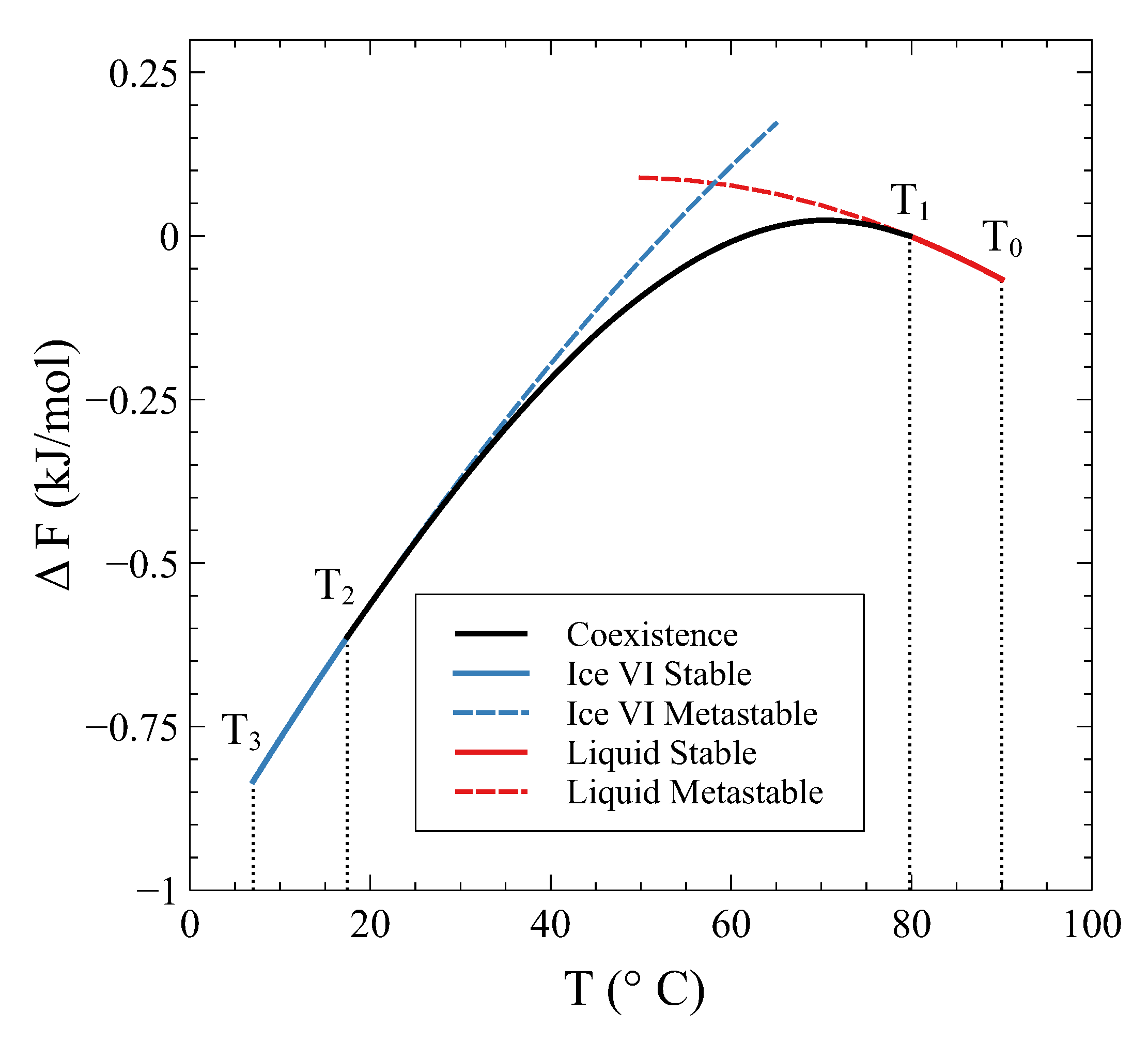
As examples, Equation (
12) can be applied to the cases of the Helmholtz potential
F and the entropy
S. For
, the contribution from the transformation is:
where we have used the equality of the chemical potentials during the transformation
. By adding the first two terms of Equation (
12), we finally obtain:
Proceeding with the entropy, from the Clapeyron equation, we obtain:
so the entropy change is:
It is easy to check that the same result is obtained by the differentiation of Equation (
14), i.e.,
. Additionally, it is interesting to note that all the previous expressions can be explicitly calculated if the quantities
,
, and
are known. In
Appendix A, the expressions for
U,
H, and
G in terms of the same quantities are given.
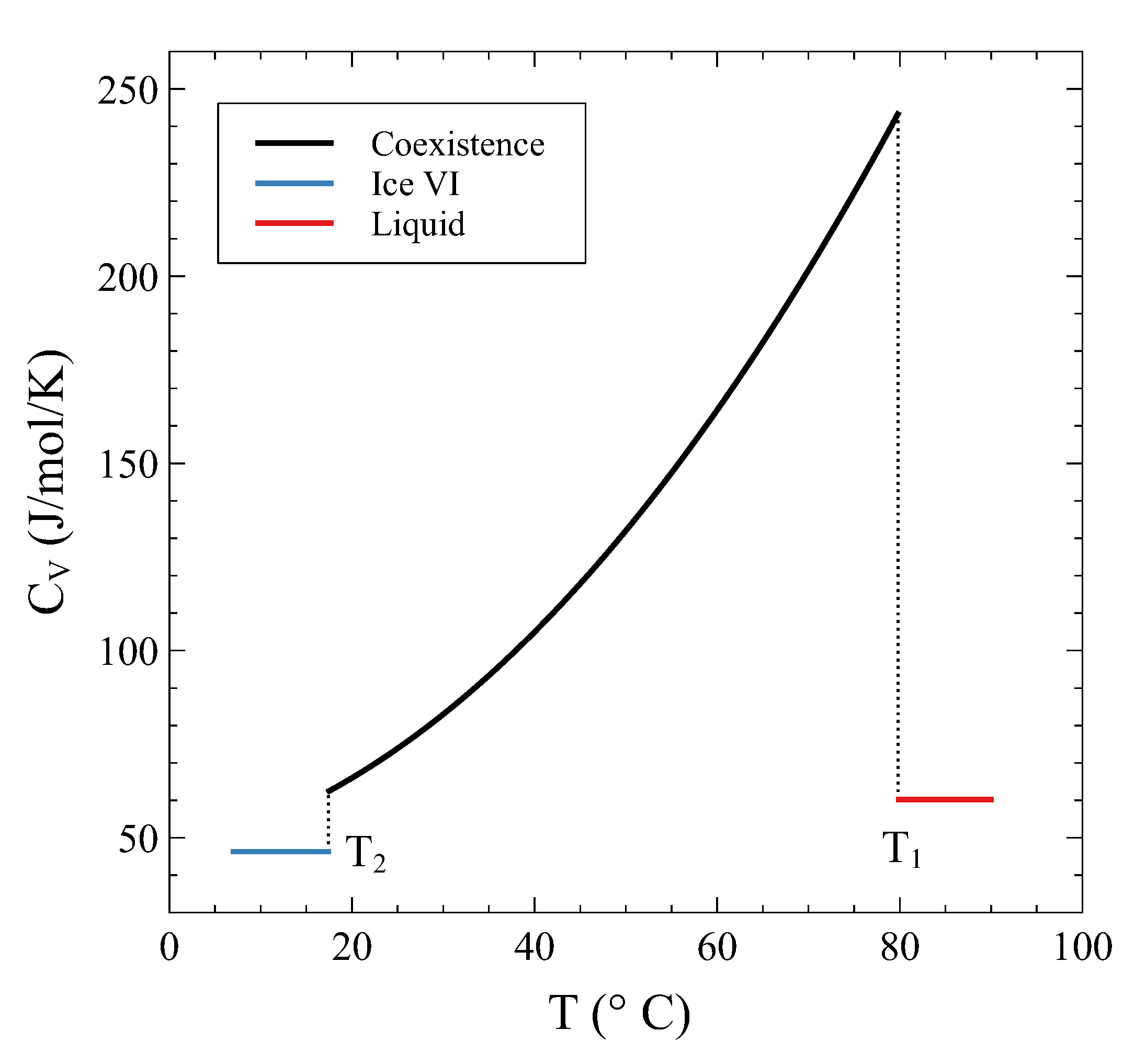
We have seen in
Section 2 that the constant pressure heat capacity exhibits a divergence during a first-order transformation at constant pressure. The analysis previously conducted on a constant volume transformation allows us to examine what happens to the heat capacity at constant volume during the isochoric transition. Contrary to what happens in a constant pressure PT, in a constant volume PT we have shown that all the thermodynamic potentials and the entropy are continuous functions across the transformation. Therefore, no divergences are expected in this case. However, there can be discrete jumps in heat capacity if different curvatures are met during the transformation.
Following Equation (
10), the heat capacity at constant volume of the whole system (
and
phases)
can be expressed as:
where
(
) are the molar specific heats for each phase at constant total volume
V (
takes into account not only the internal energy change due to a change of temperature but also the one due to a variation of
in the transformation (see
Appendix B)). After some algebra (see
Appendix B), we arrive at the following expression:
which is valid on the coexistence line.
(
) denotes the molar specific heat at constant molar volume of the
i-phase. We can evaluate this expression at the onset of the transformation,
, where
and
. As
, on the coexistence field,
. Thus:
On the other hand, as
, on the single-phase
field, the limit is trivial:
It is clear from Equations (
19) and (
20) that
is discontinuous at
(and at
, as a similar reasoning shows). Heat added to the system in the coexistence region not only is used to raise
T but to phase-transform as well. This is the origin of the discontinuity. During the constant
V transformation, as the system traverses the
coexistence line, the other susceptibilities (
,
, and
) are strictly not defined (the limits from either side do not match) or can be thought of as divergences due to the finite volume or enthalpy changes without changes in pressure or temperature. Summarizing, during the constant
V transformation, finite jumps are observed in
only when entering and leaving the coexistence region, whereas
,
, and
are not defined within the coexistence region.


