
Slow-Time Code Design for Space-Time Adaptive Processing in Airborne Radar


Abstract
:1. Introduction
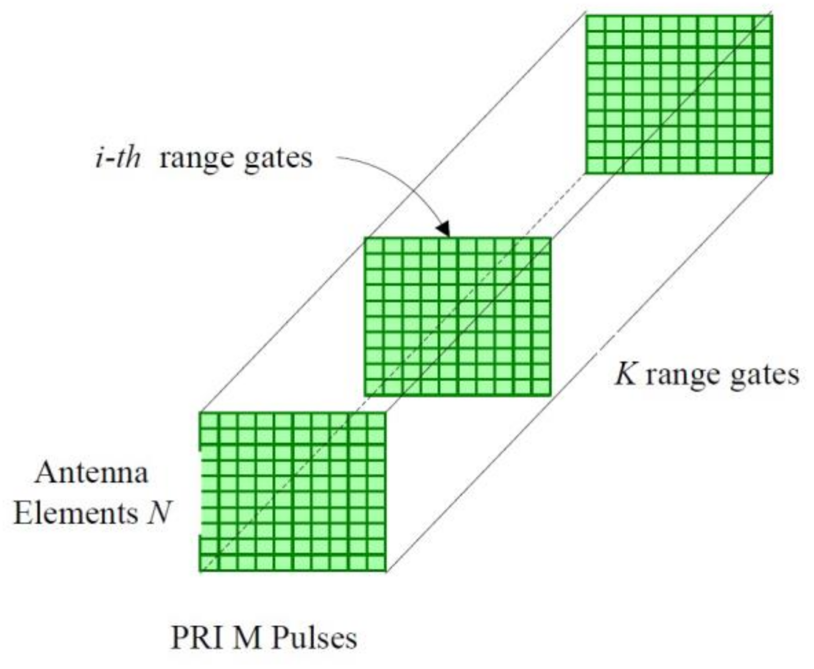
2. STAP Model
3. Slow-Time Code Design for STAP Radar
3.1. Problem Formulation
3.2. Algorithm Based on Convex Optimization
3.3. Algorithm Based on Alternating Direction Method
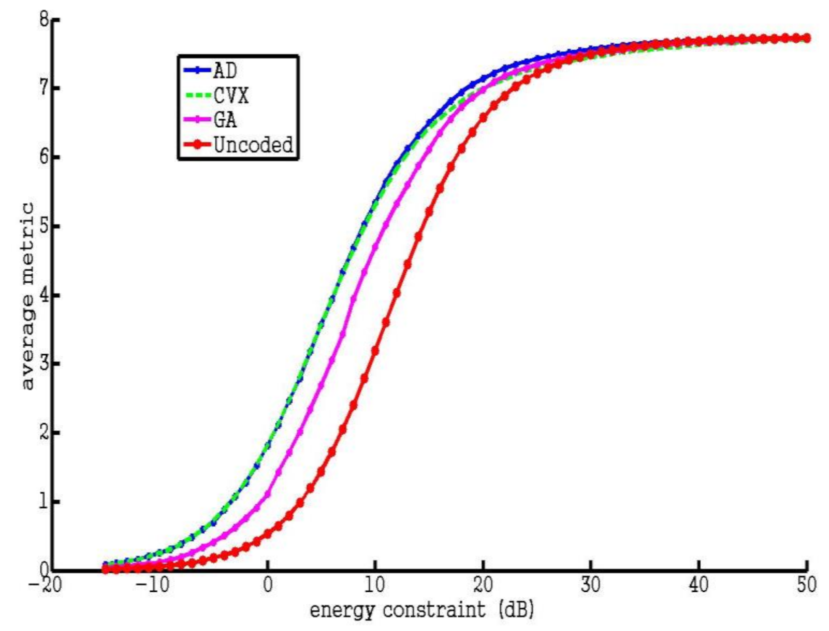
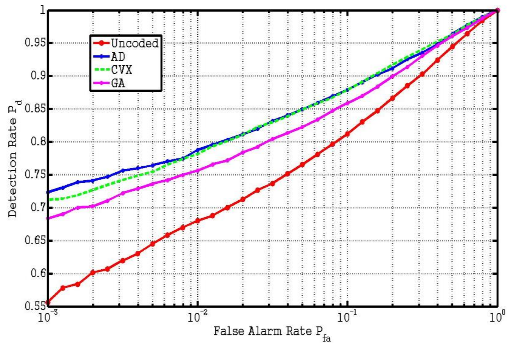
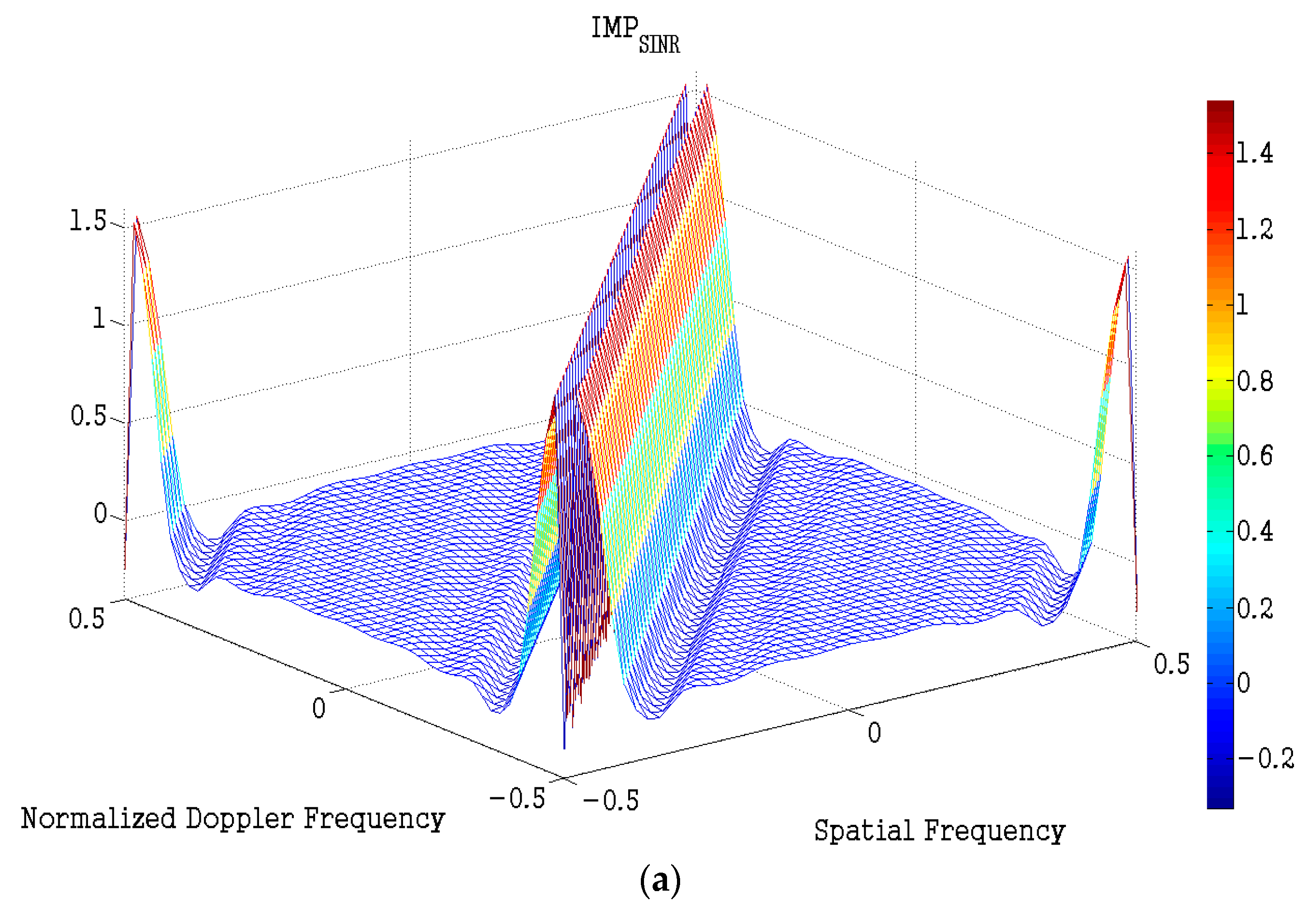
4. Numerical Examples
5. Conclusions
Author Contributions
Funding
Institutional Review Board Statement
Informed Consent Statement
Data Availability Statement
Acknowledgments
Conflicts of Interest
References
- Ward, J. Space-Time Adaptive Processing for Airborne Radar; MIT Lincoln lab.: Lexington, MA, USA, 1994. [Google Scholar]
- Klemm, R. Principle of Space-Time Adaptive Processing; IEE: Bodmin, UK, 2002. [Google Scholar]
- Grieve, P.G.; Guerci, J.R. Optimum Matched Illumination-Reception Radar. U.S. Patent S517552, 18 June 1991. [Google Scholar]
- Pillai, S.U.; OH, H.S.; Youla, D.C.; Guerci, J.R. Optimumu transmit-receiver design in the presence of signal-dependent interference and channel noise. IEEE Trans. Inf. Theory 2000, 46, 577–584. [Google Scholar] [CrossRef]
- Garren, D.A.; Osborn, M.K.; Odom, A.C.; Goldstein, J.S.; Pillai, S.U.; Guerci, J.R. Enhanced target detection and identification via optimized radar transmission pulse shape. IEEE Proc.-Radar Sonar Navig. 2001, 148, 130–138. [Google Scholar] [CrossRef]
- Zhang, J.D.; Zhu, X.H.; Wang, H.Q. Adaptive radar phase-coded wave-form design. Electron. Lett. 2009, 45, 1052–1053. [Google Scholar] [CrossRef]
- Naghibi, T.; Behnia, F. MIMO radar waveform design in the presence of clutter. IEEE Trans. Aerosp. Electron. Syst. 2011, 47, 770–781. [Google Scholar] [CrossRef]
- Setlur, P.; Rangaswamy, M. Signal dependent clutter waveform design for radar STAP. In 2014 IEEE Radar Conference; IEEE: Piscataway Township, NJ, USA, 2014; pp. 1311–1316. [Google Scholar]
- Setlur, P.; Rangaswamy, M. Projected Gradient Waveform Design for Fully Adaptive Radar STAP. In 2015 IEEE Radar Conference; IEEE: Piscataway Township, NJ, USA, 2015; pp. 1704–1709. [Google Scholar]
- Setlur, P.; Rangaswamy, M. Waveform Design for Radar STAP in Signal Dependent Interference. IEEE Trans. Signal Process. 2016, 64, 19–34. [Google Scholar] [CrossRef] [Green Version]
- Wang, H.; Cheng, Q.; Pei, B. Robust MIMO Radar Waveform Design to Improve the Worst-Case Detection Performance of STAP. IEICE Trans. Commun. 2018, 101, 1175–1182. [Google Scholar] [CrossRef]
- Li, J.; Liao, G.; Huang, Y.; Nehorai, A. Manifold Optimization for Joint Design of MIMO-STAP Radars. IEEE Signal Process. Lett. 2020, 27, 1969–1973. [Google Scholar] [CrossRef]
- Shi, S.; He, Z.; Wang, Z. Joint Design of Transmitting Waveforms and Receiving Filter for MIMO-STAP Airborne Radar. Circ. Syst. Signal Process. 2020, 39, 1489–1508. [Google Scholar] [CrossRef]
- Woodbury, M.A. Inverting Modified Matrices; Memorandum Report 42; Statistical Research Group: Princeton, NJ, USA, 1950. [Google Scholar]
- Ben-Tal, A.; Nemirovski, A. Lectures on Modern Convex Optimization; SIAM: Philadelphia, PA, USA, 2001. [Google Scholar]
- Green, B. The orthogonal approximation of an oblique structure in factor analysis. Psychometrika 1952, 17, 429–440. [Google Scholar] [CrossRef]
- Duncan, W.J. Some devices for the solution of large sets of simultaneous linear equations. Lond. Edinb. Anf. Dublin Philos. J. Sci. Seventh Ser. 1944, 35, 660–670. [Google Scholar]
- Eisen, M.; Mokhtari, A.; Ribeiro, A. Decentralized Quasi-Newton Methods. IEEE Trans. Signal Process. 2017, 65, 2613–2628. [Google Scholar] [CrossRef]
- Lellouch, G.; Mishra, A.K.; Inggs, M. Design of OFDM radar pulses using genetic algorithm based techniques. IEEE Trans. Aerosp. Electron. Syst. 2016, 52, 1953–1966. [Google Scholar] [CrossRef] [Green Version]
- Liu, B.; He, Z.; He, Q. Optimization of Orthogonal Discrete Frequency-Coding Waveform Based on Modified Genetic Algorithm for MIMO Radar. In Proceedings of the 2007 International Conference on Communications, Circuits and Systems, Kokura, Japan, 11–13 July 2007; IEEE: Piscataway, NJ, USA, 2007; pp. 966–970. [Google Scholar]
- Nayebi, M.; Aref, M.; Bastani, M. Detection of coherent radar signals with unknown Doppler shift. IEEE Proc.-Radar Sonar Navig. 1996, 143, 79–86. [Google Scholar] [CrossRef]


| Step 0: | Solve the SDP of Equation (16) to obtain . |
| Step 1: | initialize using uniform code, k = 0; |
| Step 2: | solve P1 problem by and represent the singular value decomposition (SVD) of , |
| Step 3: | solve P2 problem by , and normalized a by |
| Step 4: | set k = k + 1, repeat the steps 2∼3 until a certain stop criterion, e.g., , where is a predefined value. |
| Step 0: | initialize using uniform code, k = 0; |
| Step 1: | calculate the parameter by Equation (40); |
| Step 2: | calculate the matrix ; |
| Step 3: | set and calculate |
| Step 4: | solve problem (32) by , calculate , and normalized a by |
| Step 5: | set k = k + 1, repeat the steps 2∼4 until a certain stop criterion, e.g., , where is a predefined value. |
| Parameters | Value |
|---|---|
| Carrier frequency | 10.0 GHz |
| System bandwidth | 5 MHz |
| Pulse repetition frequency () | 5000 Hz |
| Flight velocity () | 37.5 m/s |
| Antenna array spacing () | 1.5 cm |
| Elements of antenna array N | 16 |
| Number of pulses M | 16 |
| Clutter-to-noise ratio(CNR) | 20 dB |
| Target mean power | 20 dB |
Publisher’s Note: MDPI stays neutral with regard to jurisdictional claims in published maps and institutional affiliations. |
© 2021 by the authors. Licensee MDPI, Basel, Switzerland. This article is an open access article distributed under the terms and conditions of the Creative Commons Attribution (CC BY) license (https://creativecommons.org/licenses/by/4.0/).
Share and Cite
Li, S.; Wang, N.; Zhang, J.; Xue, C.; Zhu, D. Slow-Time Code Design for Space-Time Adaptive Processing in Airborne Radar. Entropy 2021, 23, 1169. https://doi.org/10.3390/e23091169
Li S, Wang N, Zhang J, Xue C, Zhu D. Slow-Time Code Design for Space-Time Adaptive Processing in Airborne Radar. Entropy. 2021; 23(9):1169. https://doi.org/10.3390/e23091169
Chicago/Turabian StyleLi, Shiyi, Na Wang, Jindong Zhang, Chenyan Xue, and Daiyin Zhu. 2021. "Slow-Time Code Design for Space-Time Adaptive Processing in Airborne Radar" Entropy 23, no. 9: 1169. https://doi.org/10.3390/e23091169
APA StyleLi, S., Wang, N., Zhang, J., Xue, C., & Zhu, D. (2021). Slow-Time Code Design for Space-Time Adaptive Processing in Airborne Radar. Entropy, 23(9), 1169. https://doi.org/10.3390/e23091169