Extended Variational Message Passing for Automated Approximate Bayesian Inference

Abstract

Variational Message Passing (VMP) provides an automatable and efficient algorithmic framework for approximating Bayesian inference in factorized probabilistic models that consist of conjugate exponential family distributions. The automation of Bayesian inference tasks is very important since many data processing problems can be formulated as inference tasks on a generative probabilistic model. However, accurate generative models may also contain deterministic and possibly nonlinear variable mappings and non-conjugate factor pairs that complicate the automatic execution of the VMP algorithm. In this paper, we show that executing VMP in complex models relies on the ability to compute the expectations of the statistics of hidden variables. We extend the applicability of VMP by approximating the required expectation quantities in appropriate cases by importance sampling and Laplace approximation. As a result, the proposed Extended VMP (EVMP) approach supports automated efficient inference for a very wide range of probabilistic model specifications. We implemented EVMP in the Julia language in the probabilistic programming package ForneyLab.jl and show by a number of examples that EVMP renders an almost universal inference engine for factorized probabilistic models.

1. Introduction

Probabilistic Programming Languages (PPL) and packages [1] have gained strong popularity over recent years since they support fast algorithm development through automating Bayesian inference in probabilistic models. Many of these PPLs [2,3,4,5] are based on numerical approximation methods, which leads to inexact inference results, even if the model comprises conjugate factor pairs and exact inference is achievable. Moreover, although a majority of popular PPLs scale well to processing large data sets due to their stochastic inference settings [6], they tend to execute very slowly for certain types of structured dynamic models, such as state space models. Alternatively, some PPLs that execute inference by message passing in a factor graph [7,8] provide efficient inference performance by exploiting factorization and conjugacy between exponential family-based distribution pairs in the model. In particular the Variational Message Passing (VMP) [9,10] algorithm has gained a good reputation, as it supports efficient inference for conjugate factor pairs in factorized probabilistic models. Unfortunately, non-conjugate factor pairs complicate the automated estimation of posterior distributions, due to intractability of the normalization constants. Likewise, non-linear deterministic relations between model variables often create non-conjugate pairings and thus obstruct the message-passing-based inference mechanism.

This paper proposes an Extended VMP (EVMP) algorithm to support automated efficient inference on a wide class of models that contain both non-conjugate relations between factor pairs and deterministic, possibly non-linear factor nodes. In our solution proposal, the regular VMP algorithm constructs the functional forms of the messages. These functional forms contain expectations of functions of hidden variables. In the case that these expectation quantities cannot be evaluated to a closed-form expression, we estimate them by Importance Sampling (IS) [11], which is a well-known Monte Carlo method that approximates intractable posteriors by a set of weighted samples and estimates expectations over this sample set. We also make use of Laplace approximation ([12], Section 4.4) with support by automatic differentiation tools (autodiff) [13] in appropriate cases to approximate posteriors by normal distributions, which allows us to calculate the expectations over the approximating normal distribution. Our proposal leads to an efficient, automatable message-passing framework that removes most model specification limitations.

In Section 2, we start with a review of factor graphs and the VMP algorithm. Next, we specify the proposed Extended VMP algorithm in Section 3. In order to keep the paper readable, both for the advanced researcher and someone who just needs the results, we defer detailed discussions and derivations of the key equations in EVMP to Appendix A and Appendix B. We implemented EVMP in the Julia package ForneyLab.jl [8,14]. In Section 4 we present several comparative experiments of EVMP in ForneyLab vs. Turing.jl, which is an alternative state-of-the-art Julia-based PPL that focuses on Monte Carlo methods for inference. We show that EVMP transforms ForneyLab into an almost universally applicable inference engine, while retaining computational efficiency, due to its library of closed-form message passing rules. An extensive comparison to related work is presented in Section 5.

2. Problem Statement

Variational Message Passing on Forney-Style Factor Graphs

We assume a probabilistic model $p(y,z)$ with a given set of observations $y=y_{1:N}=\{y_1,\dots ,y_N\}$ and a set of latent variables $z=z_{1:M}=\{z_1,\dots ,z_M\}$. Bayesian inference in this model relates to evaluating the following posterior:

$$p\left(z\right|y)=\frac{p(y,z)}{\int p(y,z)\mathrm{d}z},$$

which relies on evaluating the model evidence $\int p(y,z)\mathrm{d}z$. Unfortunately, due to the computational complexity of evaluating the integral for the evidence, exact Bayesian inference is achievable only for a limited set of probabilistic models. Alternatively, inference can be executed by minimization of a variational objective called free energy.

$$\begin{array}{cc}\hfill \mathcal{F}\left[q\right]& ={\mathbb{E}}_q\left[log\frac{q\left(z\right)}{p(y,z)}\right]\hfill \\ \hfill & =D_{KL}\left[q\left(z\right)\right|\left|p\left(z\right|y)\right]-logp\left(y\right),\hfill \end{array}$$

(1)

where ${\mathbb{E}}_q[·]$ stands for the expectation with respect to $q\left(z\right)$ and $D_{KL}[·||·]$ denotes a Kullback–Leibler divergence. (In this paper, we denote the expected value $\int q\left(x\right)f\left(x\right)\mathrm{d}x$ of function f with respect to distribution q both by $E_q\left[f\left(x\right)\right]$ and ${〈f\left(x\right)〉}_q$.) The KL divergence is greater or equal to zero for any distribution $q\left(z\right)$ and $D_{KL}\left[q\left(z\right)\right|\left|p\left(z\right|y)\right]=0$ if and only if $q\left(z\right)=p\left(z\right|y)$. As a result, minimizing the free energy with respect to q leads both to an approximate posterior

$$q^{\ast }\left(z\right)=arg\underset{q}{max}\mathcal{F}\left[q\right]\approx p\left(z\right|y)$$

and an upper bound $\mathcal{F}\left[q^{\ast }\right]$ on the negative log-evidence. In practice, minimization of $\mathcal{F}$ is often greatly alleviated by assuming a mean-field constraint, i.e., a fully factorized posterior $q\left(z_{1:M}\right)={\displaystyle \prod _{i=1}^M}q\left(z_i\right)$.

Variational inference on factorized models $p(y,z)$ with the mean-field assumption for q leads to an automatable algorithm called Variational Message Passing (VMP) [9,10]. VMP can be visualized by representing the model as a graph and interpreting the VMP update equations as messages.

In this paper, we favor a Forney-style Factor Graph (FFG) representation to visualize the factorization properties of probabilistic models and inference by message passing [15]. FFGs are undirected graph representations of factorized probabilistic models in which the conditional distributions are represented by nodes and the variables are associated with edges that connect the nodes. Besides visualizing the factorization properties of probabilistic models, FFGs also provide a formal framework for message passing-based inference in probabilistic models. In the FFGs that we discuss here, we distinguish three types of factors (nodes): soft factors, deterministic factors and equality factors. Throughout the paper, a soft factor represents an Exponential Family (EF) distribution (see (6) for definition) such as a Gaussian, Bernoulli, Gamma or Categorical distribution. Deterministic factors hold deterministic mappings of variables; in particular, we will use the relation $f_{\delta }(x,z)=p\left(x\right|z)=\delta (x-g\left(z\right))$, where $g(·)$ is a deterministic function. Lastly, equality factors are used to circumvent the constraint that an edge (representing a variable z) can only be connected to maximally two factors. In an FFG representation, this problem is resolved by adding variable copies $z^{\prime }$ and $z^{″}$ and constraining the beliefs over these copy variables through an equality factor $f_{=}(z,z^{\prime },z^{″})=\delta (z-z^{\prime })\delta (z-z^{″})$. As an example, the FFG for one time step for a hierarchical state-space model is visualized in Figure 1. In this graph, the factors $f_a(z_t^{\prime },z_{t-1})=p\left(z_t^{\prime }\right|z_{t-1})$, $f_b(x_t^{\prime },x_{t-1},w_t)=p\left(x_t^{\prime }\right|x_{t-1},w_t)$, $f_c(y_t,x_t^{″})=p\left(y_t\right|x_t^{″})$ are encoded by EF distributions. The factor $f_{\delta }(w_t,z_t^{″})=p\left(w_t\right|z_t^{″})=\delta (w_t-g\left(z_t^{″}\right))$, for a given function $g(·)$, represents a non-linear deterministic relation. An interesting property of FFGs is the hierarchical composition: we can create new “higher level” nodes by enclosing a set of connected nodes in a box and integrating out the internal variables in the box. For instance, the composite node $f_d$ can be created through the following:

$$\begin{array}{cc}\hfill f_d(x_t^{\prime },x_{t-1},z_t^{″})& =p\left(x_t^{\prime }\right|x_{t-1},z_t^{″})\hfill \\ \hfill & =\int p\left(x_t^{\prime }\right|x_{t-1},w_t)\delta (w_t-g\left(z_t^{″}\right))\mathrm{d}{w}_t\hfill \\ \hfill & =\int f_b(x_t^{\prime },x_{t-1},w_t)f_{\delta }(w_t,z_t^{″})\mathrm{d}{w}_t\hfill \end{array}$$

For a more detailed introduction to FFGs, we refer to [15,16].

Aside from visualization, FFGs also serve to formalize message-passing-based inference in probabilistic models, and VMP on FFGs realizes coordinate-descent optimization of the free energy functional (1). Coordinate-descent optimization of the free energy refers to iterative updates of the variational factors one at a time while keeping the other factors fixed [12,17]. To illustrate, let us optimize $\mathcal{F}$ with respect to $q\left(z_k\right)$ for the system $f_a\left(z_{1:k}\right)f_b\left(z_{k:K}\right)$ (see Figure 2). First, we decompose the free energy as follows:

$$\begin{array}{c}\hfill \mathcal{F}=\tilde{\mathcal{F}}+\underset{{\mathcal{F}}_k}{\underbrace{{\mathbb{E}}_{q\left(z_{1:K}\right)}\left[log\frac{q\left(z_k\right)}{f_a\left(z_{1:k}\right)f_b\left(z_{k:K}\right)}\right]}},\end{array}$$

where $\tilde{\mathcal{F}}$ holds terms that are not a function of variable $z_k$. The term ${\mathcal{F}}_k$ can be re-arranged as follows:

$$\begin{array}{cc}\hfill {\mathcal{F}}_k& ={\mathbb{E}}_{q\left(z_k\right)}\left[log\frac{q\left(z_k\right)}{exp\left({\mathbb{E}}_{q\left(z_{1:k-1}\right)}[log{f}_a\left(z_{1:k}\right)]\right)exp\left({\mathbb{E}}_{q\left(z_{k+1:K}\right)}[log{f}_b\left(z_{k:K}\right)]\right)}\right],\hfill \end{array}$$

(2)

so it follows that ${\mathcal{F}}_k$ is minimized when $q\left(z_k\right)$ is set proportional to the denominator in (2) [12,17]. In addition, notice that the terms with the local factors $f_a$ and $f_b$ are uncoupled, which paves the way for a message-passing interpretation of coordinate-descent variational inference. As a result, provided that $f_a$ and $f_b$ are not deterministic factors, the VMP algorithm proceeds by repeating the following four steps until convergence [10]:

• Choose a variable $z_k$ from the set $z_{1:K}$.
• Compute the incoming messages.

  $$\begin{gathered} \begin{array}{cc}\hfill {\overrightarrow{m}}_{z_k}\left(z_k\right)& \propto exp\left({〈log{f}_a\left(z_{1:k}\right)〉}_{q\left(z_{1:k-1}\right)}\right)\hfill \end{array} \\ \begin{array}{cc}\hfill {\overleftarrow{m}}_{z_k}\left(z_k\right)& \propto exp\left({〈log{f}_b\left(z_{k:K}\right)〉}_{q\left(z_{k+1:K}\right)}\right)\hfill \end{array} \end{gathered}$$

  (3)
• Update the posterior.

  $$\begin{array}{c}\hfill q\left(z_k\right)=\frac{{\overrightarrow{m}}_{z_k}\left(z_k\right){\overleftarrow{m}}_{z_k}\left(z_k\right)}{\int {\overrightarrow{m}}_{z_k}\left(z_k\right){\overleftarrow{m}}_{z_k}\left(z_k\right)\mathrm{d}{z}_k}.\end{array}$$

  (4)
• Update the local free energy (for performance tracking), i.e., update all terms in $\mathcal{F}$ that are affected by the update (4):

  $$\begin{array}{c}\hfill {\mathcal{F}}_k={〈log\frac{q\left(z_k\right)}{f_a\left(z_{1:k}\right)f_b\left(z_{k:K}\right)}〉}_{q\left(z_{1:K}\right)}.\end{array}$$

  (5)

As we see in (3), messages flow on edges in both directions. It is common parlance to call one of the messages the forward message (denoted by ${\overrightarrow{m}}_{z_k}\left(z_k\right)$) and the other the backward message (${\overleftarrow{m}}_{z_k}\left(z_k\right)$).

In this paper, the central problem is how to execute the VMP update Equation (3) through (5) for a wide range of specifications for the factors $f_a$ and $f_b$. In the next section, we specify the proposed Extended VMP (EVMP) solution. A more detailed derivation of the key equations of EVMP is provided in Appendix B.

3. Specification of EVMP Algorithm

Variational Message Passing is a fast, efficient and deterministic approximate inference algorithm. However, the applicability of VMP heavily relies on connected factors being conjugate pairs (see Appendix A). In contrast, Monte Carlo methods (see [18] for message-passing interpretation) are applicable to a wider range of models with non-conjugate factor pairs. Unfortunately, in comparison to VMP, Monte Carlo methods are considerably slower since they rely on stochastic simulations. As we elaborate in Section 5, the recent efforts to combine the best of Monte Carlo methods and variational inference predominantly focus on noisy gradient estimation of the free energy through Monte Carlo sampling and do not take the full advantage of deterministic message passing steps in inference.

In this section, we specify the EVMP algorithm, which combines the efficiency of VMP with the flexibility of the Laplace approximation and the universality of Monte Carlo methods. In the proposed EVMP algorithm, VMP constructs the functional forms of the messages while importance sampling and Laplace approximations are used to estimate the required expectations of statistical quantities if they are not available in closed form. We first specify the range of probability distribution types for factors, messages and posteriors. These different types are used to identify the specific calculation rules for updating the messages and posteriors in (3) and (4). We refer the interested reader to Appendix B for detailed derivations.

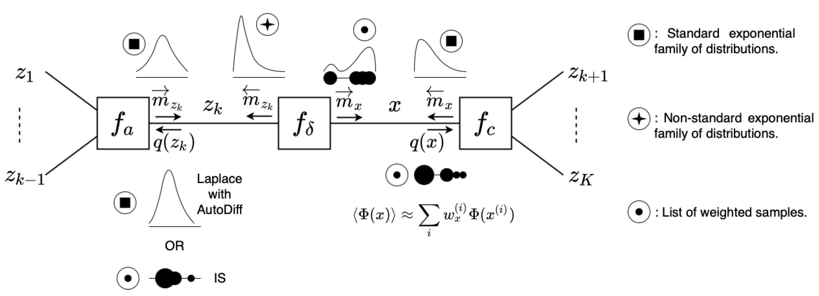
3.1. Distribution Types

We consider the following representation types for probability distributions in factors $p\left(z\right)$, where z holds a variable.

(1)

The standard Exponential Family (EF) of distributions, i.e., the following:

$$p\left(z\right)=h\left(z\right)exp\left(\varphi {\left(z\right)}^{⊺}\eta -A_{\eta }\left(\eta \right)\right),$$

(6)

where $h\left(z\right)$ is the base measure, $\varphi \left(z\right)$ is the sufficient statistics vector, $\eta$ is the natural parameters vector and $A_{\eta }\left(\eta \right)$ is the log-partition function.

(2)

Distributions that are of the following exponential form:

$$p\left(z\right)\propto exp\left(\varphi {\left(g\left(z\right)\right)}^{⊺}\eta \right),$$

(7)

where $g\left(z\right)$ is a deterministic function. The key characteristic here is that $\varphi \left(g\right(z\left)\right)$ is not recognized as a sufficient statistics vector for any of the standard EF distributions. We call this distribution type a Non-Standard Exponential Family (NEF) distribution. As we show in Section 3.6, this distribution type arises only in backward message calculations.

(3)

A List of Weighted Samples (LWS), i.e., the following:

$$p\left(z\right):=\left\{\left(w^{\left(1\right)},z^{\left(1\right)}\right),\dots ,\left(w^{\left(N\right)},z^{\left(N\right)}\right)\right\}.$$

(8)

(4)

Deterministic relations are represented by delta distributions, i.e., the following:

$$p\left(x\right|z)=\delta (x-g\left(z\right)).$$

(9)

Technically, the equality factor $f(x,y,z)=\delta (z-x)\delta (z-y)$ also specifies a deterministic relation between variables.

3.2. Factor Types

Factor types $f\left(z\right)$ are represented by EF and delta distributions.

In a VMP setting, as discussed in this and previous papers on VMP, conjugate soft factors from the exponential family enjoy some computational advantages. As an extension to VMP, the EVMP algorithm inherits the same computational advantages for conjugate factor pairs. In order to automate and generalize the inference to custom non-conjugate soft factors, we compose a generic soft factor by a delta distribution (to describe a non-linear deterministic function) and a standard EF distribution. This decomposition relieves us from manually deriving VMP messages for each different soft factor specification. For a given composite node (delta + standard EF), the EVMP algorithm uses the predefined VMP messages for the standard EF component to compute messages around the composite node. As we will see, this formulation yields an almost generic inference procedure.

3.3. Message Types

Forward messages carry either an EF or an LWS distribution. Backward messages carry either an EF or an NEF distribution. This is an arbitrary choice in the sense that we only make this assignment to indicate that in the EVMP algorithm, two colliding messages in posterior calculations are not both of the LWS type nor both of the NEF type.

3.4. Posterior Types

The posteriors $q\left(z\right)$ are represented by either the EF or LWS representations.

To summarize the terminology so far, we defined four distribution types: Standard EF (EF), Non-Standard EF (NEF), List of Weighted Samples (LWS) and delta distributions. The end user of our algorithm can design a model by using EF and delta distributions. Under the hood, messages may carry EF, NEF or LWS distributions to render the inference. As the output, the end user is provided with either the EF or LWS posteriors. Next, we discuss how posteriors, messages and free energies are computed in the EVMP algorithm. The different types can be used to identify which computational recipe applies. As an aside, Julia’s support for multiple dispatch in functions [14] makes this a very elegant mechanism that requires almost no if–then rules.

3.5. Computation of Posteriors

Here, we discuss how EVMP updates the posteriors in (4). In an FFG, computation of the posterior $q\left(z\right)$ is realized by a multiplication of colliding forward and backward messages, respectively ${\overrightarrow{m}}_z\left(z\right)$ and ${\overleftarrow{m}}_z\left(z\right)$, followed by normalization. We distinguish four types of updates.

(1)

In the case that the colliding forward and backward messages both carry EF distributions with the same sufficient statistics $\varphi \left(z\right)$, then computing the posterior simplifies to a summation of natural parameters:

$$\begin{array}{cc}\hfill {\overrightarrow{m}}_z\left(z\right)& \propto exp\left(\varphi {\left(z\right)}^{⊺}{\eta }_1\right)\hfill \\ \hfill {\overleftarrow{m}}_z\left(z\right)& \propto exp\left(\varphi {\left(z\right)}^{⊺}{\eta }_2\right)\hfill \\ \hfill q\left(z\right)& \propto {\overrightarrow{m}}_z\left(z\right)·{\overleftarrow{m}}_z\left(z\right)\propto exp\left(\varphi {\left(z\right)}^{⊺}({\eta }_1+{\eta }_2)\right).\hfill \end{array}$$

In this case, the posterior $q\left(z\right)$ will also be represented by the EF distribution type. This case corresponds to classical VMP with conjugate factor pairs.

(2)

The forward message again carries a standard EF distribution. The backward message carries either an NEF distribution or a non-conjugate EF distribution.

(a)

If the forward message is Gaussian, i.e., ${\overrightarrow{m}}_z\left(z\right)=\mathcal{N}(z;{\mu }_1,V_1)$, we use a Laplace approximation to compute the posterior:

$$\begin{array}{cc}\hfill \mu & =arg\underset{z}{max}\left(log{\overrightarrow{m}}_z\left(z\right)+log{\overleftarrow{m}}_z\left(z\right)\right),\hfill \\ \hfill V& ={(-\nabla {\nabla }_z(log{\overrightarrow{m}}_z\left(z\right)+log{\overleftarrow{m}}_z\left(z\right)){|}_{z=\mu })}^{-1}\hfill \\ \hfill q\left(z\right)& \propto {\overrightarrow{m}}_z\left(z\right)·{\overleftarrow{m}}_z\left(z\right)=\mathcal{N}(z;\mu ,V)\hfill \end{array}$$

(10)

(b)

Otherwise (${\overrightarrow{m}}_z\left(z\right)$ is not a Gaussian), we use Importance Sampling (IS) to compute the posterior:

$$\begin{array}{cc}\hfill z^{\left(1\right)},\dots ,z^{\left(N\right)}& \sim {\overrightarrow{m}}_z\left(z\right),\hfill \\ \hfill {\tilde{w}}^{\left(i\right)}& ={\overleftarrow{m}}_z\left(z^{\left(i\right)}\right)\mathrm{for}i=1,\dots ,N\hfill \\ \hfill w^{\left(i\right)}& ={\tilde{w}}^{\left(i\right)}/\sum _{j=1}^N{\tilde{w}}^{\left(j\right)}\mathrm{for}i=1,\dots ,N\hfill \\ \hfill q\left(z\right)& \propto {\overrightarrow{m}}_z\left(z\right)·{\overleftarrow{m}}_z\left(z\right)=\left\{\left(w^{\left(1\right)},z^{\left(1\right)}\right),\dots ,\left(w^{\left(N\right)},z^{\left(N\right)}\right)\right\}.\hfill \end{array}$$

(11)

(3)

The forward message carries an LWS distribution, i.e., the following:

$${\overrightarrow{m}}_z\left(z\right):=\left\{\left(w_1^{\left(1\right)},z_1^{\left(1\right)}\right),\dots ,\left(w_1^{\left(N\right)},z_1^{\left(N\right)}\right)\right\},$$

and the backward message carries either an EF or NEF distribution. In that case, the posterior computation refers to updating the weights in ${\overrightarrow{m}}_z\left(z\right)$ (see Appendix E):

$$\begin{array}{cc}\hfill {\tilde{w}}^{\left(i\right)}& =w_1^{\left(i\right)}{\overleftarrow{m}}_z\left(z_1^{\left(i\right)}\right)\mathrm{for}i=1,\dots ,N\hfill \\ \hfill w^{\left(i\right)}& ={\tilde{w}}^{\left(i\right)}/\sum _{j=1}^N{\tilde{w}}^{\left(j\right)}\mathrm{for}i=1,\dots ,N\hfill \\ \hfill z^{\left(1\right)},\dots ,z^{\left(N\right)}& =z_1^{\left(1\right)},\dots ,z_1^{\left(N\right)}\hfill \\ \hfill q\left(z\right)& \propto {\overrightarrow{m}}_z\left(z\right)·{\overleftarrow{m}}_z\left(z\right)=\left\{\left(w^{\left(1\right)},z^{\left(1\right)}\right),\dots ,\left(w^{\left(N\right)},z^{\left(N\right)}\right)\right\}.\hfill \end{array}$$

(12)

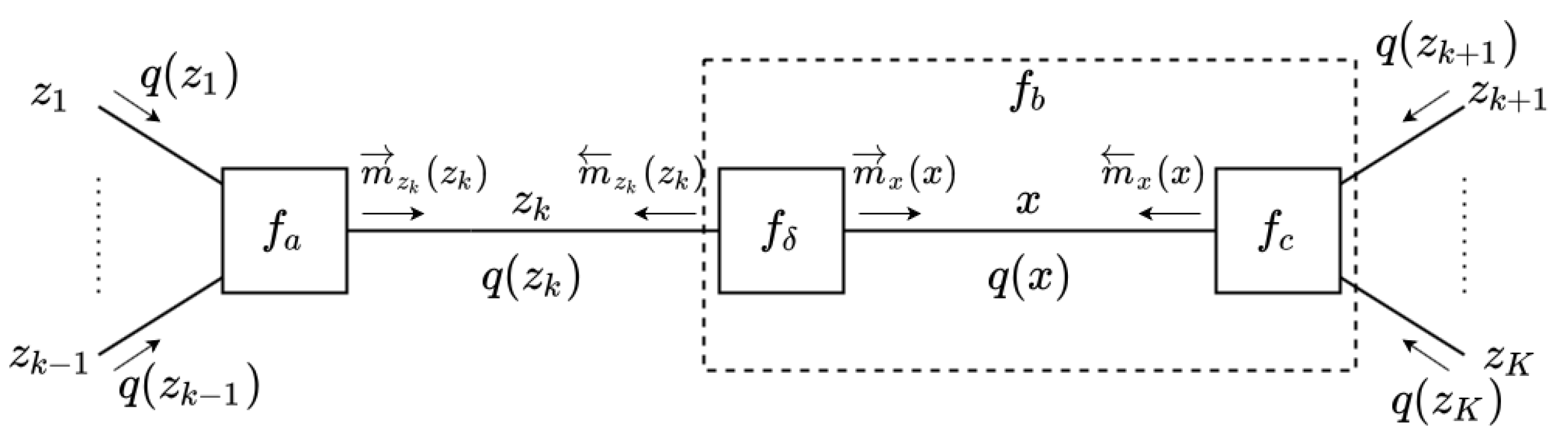
3.6. Computation of Messages

Here, we discuss how EVMP compute the messages (3). We specify different message calculation rules depending of the type of the factor.

(1)

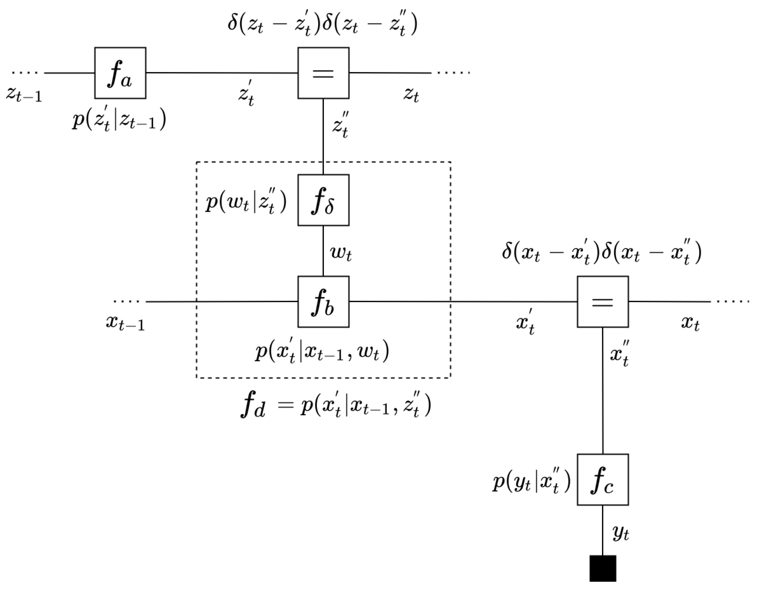
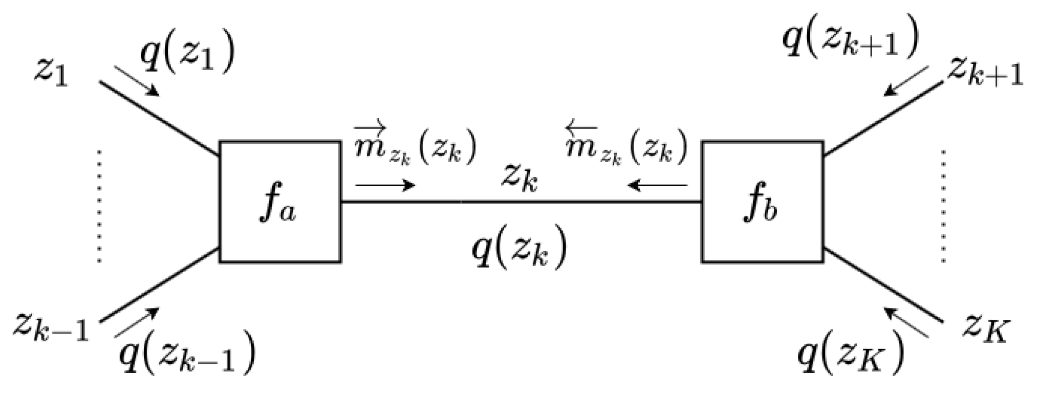
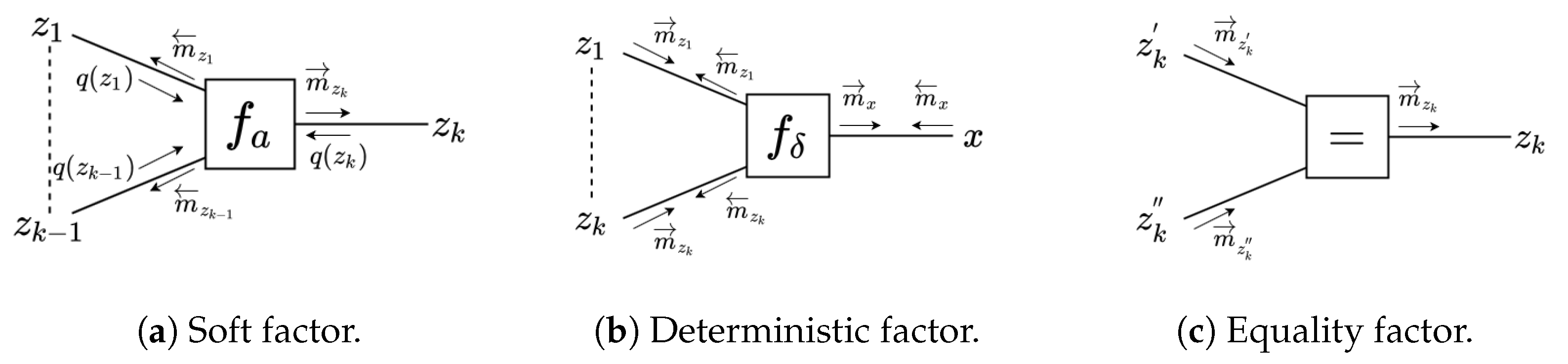
If factor $f_a(z_1,z_2,\dots ,z_k)$ is a soft factor of the form (see Figure 3a)

$$\begin{array}{c}\hfill f_a\left(z_{1:k}\right)=p\left(z_k\right|z_{1:k-1})=h_a\left(z_k\right)exp\left({\varphi }_a{\left(z_k\right)}^{⊺}{\eta }_a\left(z_{1:k-1}\right)-A_a\left(z_{1:k-1}\right)\right).\end{array}$$

then the outgoing VMP message to $z_k$ is the following EF-distributed message:

$$\begin{array}{cc}\hfill {\overrightarrow{m}}_{z_k}\left(z_k\right)& \propto h_a\left(z_k\right)exp\left({\varphi }_a{\left(z_k\right)}^{⊺}{〈{\eta }_a\left(z_{1:k-1}\right)〉}_{q\left(z_{1:k-1}\right)}\right).\hfill \end{array}$$

(13)

If rather $z_1$ (or $z_2,\dots ,z_{k-1}$) than $z_k$ is the output variable of $f_a$, i.e., if the following is true:

$$\begin{array}{c}\hfill f_a\left(z_{1:k}\right)=p\left(z_1\right|z_{2:k})=h_a\left(z_1\right)exp\left({\varphi }_a{\left(z_1\right)}^{⊺}{\eta }_a\left(z_{2:k}\right)-A_a\left(z_{2:k}\right)\right).\end{array}$$

then the outgoing message to $z_k$ is either an EF or an NEF distribution of the following form:

$$\begin{array}{cc}\hfill {\overleftarrow{m}}_{z_k}\left(z_k\right)& \propto exp\left({〈{\varphi }_a\left(z_1\right)〉}_{q\left(z_1\right)}^{⊺}{〈{\eta }_a\left(z_{2:k}\right)〉}_{q\left(z_{2:k-1}\right)}-{〈A_a\left(z_{2:k}\right)〉}_{q\left(z_{2:k-1}\right)}\right).\hfill \end{array}$$

(14)

In this last expression, we chose to assign a backward arrow to ${\overleftarrow{m}}_{z_k}\left(z_k\right)$ since it is customary to align the message direction with the direction of the factor, which in this case points to $z_1$.

Note that the message calculation rule for ${\overrightarrow{m}}_{z_k}\left(z_k\right)$ requires the computation of expectation ${〈{\eta }_a\left(z_{1:k-1}\right)〉}_{q\left(z_{1:k-1}\right)}$, and for ${\overleftarrow{m}}_{z_k}\left(z_k\right)$ we need to compute expectations ${〈{\varphi }_a\left(z_1\right)〉}_{q\left(z_1\right)}$ and ${〈{\eta }_a\left(z_{2:k}\right)〉}_{q\left(z_{2:k-1}\right)}$. In the update rules to be shown below, we will see these expectations of statistics of z appear over and again. In Section 3.8 we detail how we calculate these expectations and in Appendix A, we further discuss the origins of these expectations.

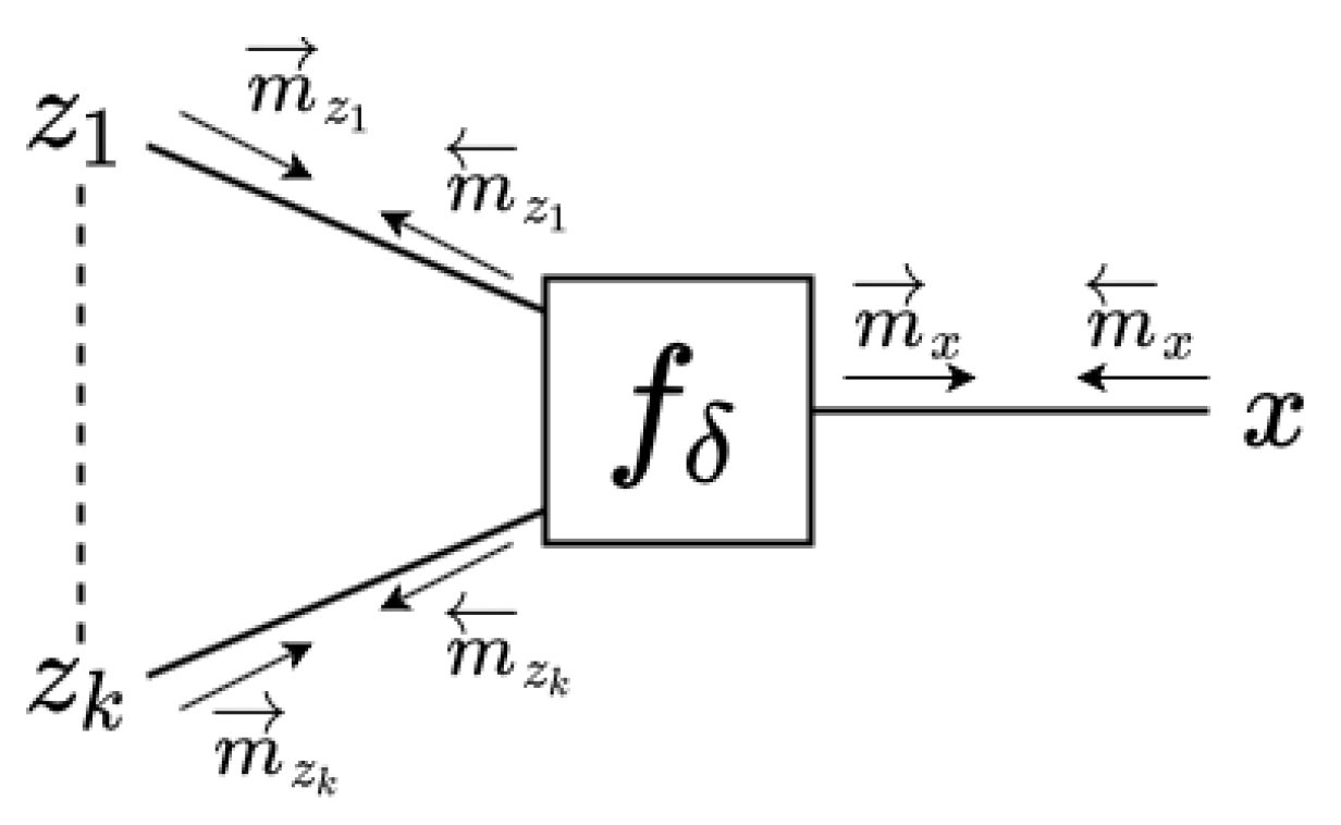
(2)

In the case that $f_{\delta }$ is a deterministic factor (see Figure 3b):

$$\begin{array}{c}\hfill f_{\delta }(x,z_{1:k})=p\left(x\right|z_{1:k})=\delta (x-g\left(z_{1:k}\right)).\end{array}$$

(15)

then the forward message from $f_{\delta }$ to x is of LWS type and is calculated as follows:

$$\begin{array}{cc}\hfill & {\overrightarrow{m}}_x\left(x\right)=\left\{\left(\frac{1}{N},g\left(z_{1:k}^{\left(1\right)}\right)\right),\dots ,\left(\frac{1}{N},g\left(z_{1:k}^{\left(N\right)}\right)\right)\right\},\hfill \\ & \mathrm{where}{z}_j^{\left(i\right)}\sim {\overrightarrow{m}}_{z_j}\left(z_j\right)\mathrm{for}j=1:k.\hfill \end{array}$$

(16)

For the computation of the backward message toward $z_k$, we distinguish two cases:

(a)

If all forward incoming messages from the variables $z_{1:k}$ are Gaussian, we first use a Laplace approximation to obtain a Gaussian joint posterior $q\left(z_{1:k}\right)=\mathcal{N}(z_{1:k};{\mu }_{1:k},V_{1:k})$; see Appendix B.1.2 and Appendix B.2.2 for details. Then, we evaluate the posteriors for individual random variables, e.g., $q\left(z_k\right)=\int q\left(z_{1:k}\right)\mathrm{d}{z}_{1:k-1}=\mathcal{N}(z_k;{\mu }_k,V_k)$. Finally, we send the following Gaussian backward message:

$$\begin{array}{c}\hfill {\overleftarrow{m}}_{z_k}\left(z_k\right)\propto q\left(z_k\right)/{\overrightarrow{m}}_{z_k}\left(z_k\right).\end{array}$$

(17)

(b)

Otherwise (the incoming messages from the variables $z_{1:k}$ are not all Gaussian), we use Monte Carlo and send a message to $z_k$ as a NEF distribution:

$$\begin{array}{c}\hfill {\overleftarrow{m}}_{z_k}\left(z_k\right)\approx \frac{1}{N}\sum _{i=1}^N{\overleftarrow{m}}_x\left(g(z_{1:k-1}^{\left(i\right)},z_k)\right),\mathrm{where}{z}_j^{\left(i\right)}\sim {\overrightarrow{m}}_{z_j}\left(z_j\right).\end{array}$$

(18)

Note that if $f_{\delta }$ is a single input deterministic node, i.e., $f_{\delta }(x,z_k)=p\left(x\right|z_k)=\delta (x-g\left(z_k\right))$, then the backward message simplifies to ${\overleftarrow{m}}_{z_k}\left(z_k\right)={\overleftarrow{m}}_x\left(g\left(z_k\right)\right)$ (Appendix B.1.1).

(3)

The third factor type that leads to a special message computation rule is the equality node; see Figure 3c. The outgoing message from an equality node

$$f_{=}(z,z^{\prime },z^{″})=\delta (z-z^{\prime })\delta (z-z^{″})$$

is computed by following the sum–product rule:

$$\begin{array}{cc}\hfill {\overrightarrow{m}}_{z_k}\left(z_k\right)& =\int \underset{\mathrm{node}\mathrm{function}}{\underbrace{\delta (z_k-z_k^{\prime })\delta (z_k-z_k^{″})}}\underset{\mathrm{incoming}\mathrm{messages}}{\underbrace{{\overrightarrow{m}}_{z_k^{\prime }}\left(z_k^{\prime }\right){\overrightarrow{m}}_{z_k^{″}}\left(z_k^{″}\right)}}\mathrm{d}{z}_k^{\prime }\mathrm{d}{z}_k^{″}\hfill \\ \hfill & ={\overrightarrow{m}}_{z_k^{\prime }}\left(z_k\right){\overrightarrow{m}}_{z_k^{″}}\left(z_k\right).\hfill \end{array}$$

(19)

3.7. Computation of Free Energy

Here, we discuss how EVMP computes the FE update from (5). Note that the FE can be decomposed into a subtraction of energy and entropy terms:

$$\begin{array}{cc}\hfill {\mathcal{F}}_k& ={〈log\frac{q\left(z_k\right)}{f_a\left(z_{1:k}\right)f_b\left(z_{k:K}\right)}〉}_{q\left(z_{1:K}\right)}\hfill \\ \hfill & =\underset{\left(\mathrm{average}\right)\mathrm{energy}{\mathcal{U}}_a+{\mathcal{U}}_b}{\underbrace{{〈log\frac{1}{f_a\left(z_{1:k}\right)f_b\left(z_{k:K}\right)}〉}_{q\left(z_{1:K}\right)}}}-\underset{\mathrm{entropy}{\mathcal{H}}_k}{\underbrace{{〈log\frac{1}{q\left(z_k\right)}〉}_{q\left(z_k\right)}}}\hfill \end{array}$$

(20)

These energy and entropy terms can be evaluated because $f_a\left(z_{1:k}\right)f_b\left(z_{k:K}\right)$ contains only factors that are defined in the generative model and $q\left(z_{1:K}\right)$ is also accessible as a result of variational inference. Thus, we evaluate the FE by evaluating the energy and entropy terms separately.

For an EF-encoded soft factor

$$f_a\left(z_{1:k}\right)=p\left(z_k\right|z_{1:k-1})=h_a\left(z_k\right)exp\left({\varphi }_a{\left(z_k\right)}^{⊺}{\eta }_a\left(z_{1:k-1}\right)-A_{\eta }\left({\eta }_a\left(z_{1:k-1}\right)\right)\right),$$

the energy over the factor $f_a$ evaluates to

$$\begin{array}{cc}\hfill {\mathcal{U}}_a& =-{〈log\left(f_a\left(z_{1:k}\right)\right)〉}_{q\left(z_{1:k}\right)}\hfill \\ \hfill & =-{〈log\left(h_a\left(z_k\right)\right)〉}_{q\left(z_k\right)}-{〈{\varphi }_a\left(z_k\right)〉}_{q\left(z_k\right)}^{⊺}{〈{\eta }_a\left(z_{1:k-1}\right)〉}_{q\left(z_{1:k-1}\right)}+{〈A_{\eta }\left({\eta }_a\left(z_{1:k-1}\right)\right)〉}_{q\left(z_{1:k-1}\right)}.\hfill \end{array}$$

The entropy terms only need to be evaluated for variables z that are not associated with output edges of deterministic nodes. In that case, we calculate the entropy of $q\left(z\right)$ as follows:

• If $q\left(z\right)$ is a represented by a standard EF distribution, i.e.,

  $$q\left(z\right)=h\left(z\right)exp\left(\varphi {\left(z\right)}^{⊺}\eta -A_{\eta }\left(\eta \right)\right),$$

  then

  $$\begin{array}{c}\hfill {\mathcal{H}}_z=-{〈log\left(h\right(z\left)\right)〉}_{q\left(z\right)}-{〈\varphi \left(z\right)〉}_{q\left(z\right)}^{⊺}\eta +A_{\eta }\left(\eta \right).\end{array}$$
• Otherwise, if $q\left(z\right)$ is represented by a LWS, i.e.,

  $$q\left(z\right):=\left\{\left(w^{\left(1\right)},z^{\left(1\right)}\right),\dots ,\left(w^{\left(N\right)},z^{\left(N\right)}\right)\right\},$$

  then

  $$\begin{array}{c}\hfill {\mathcal{H}}_z={\widehat{\mathcal{H}}}_z^1+{\widehat{\mathcal{H}}}_z^2,\end{array}$$

  where ${\widehat{\mathcal{H}}}_z^1$ and ${\widehat{\mathcal{H}}}_z^2$ are evaluated as discussed in (A43) and (A45).

3.8. Expectations of Statistics

In many of the above computations for messages, posteriors and free energies, we need to compute certain expectations of statistics of z, e.g., the computation of the forward message in (13) requires evaluation of ${〈{\eta }_a\left(z_{1:k-1}\right)〉}_{q\left(z_{1:k-1}\right)}$. Here, we discuss how EVMP evaluates these expectations. Let us denote a statistic of random variable z by $\Phi \left(z\right)$ and assume we are interested in the expected value ${〈\Phi \left(z\right)〉}_{q\left(z\right)}$. The calculation rule depends on the type of $q\left(z\right)$:

(1)

We have two cases when $q\left(z\right)$ is coded as an EF distribution, i.e.,

$$q\left(z\right)=h\left(z\right)exp\left(\varphi {\left(z\right)}^{⊺}\eta -A_{\eta }\left(\eta \right)\right):$$

(a)

If $\Phi \left(z\right)\in \varphi \left(z\right)$, i.e., the statistic $\Phi \left(z\right)$ matches with elements of the sufficient statistics vector $\varphi \left(z\right)$, then ${〈\Phi \left(z\right)〉}_{q\left(z\right)}$ is available in closed form as the gradient of the log-partition function (this is worked out in Appendix A.1.1, see (A14) and (A15)):

$${〈\Phi \left(z\right)〉}_{q\left(z\right)}\in {\nabla }_{\eta }{A}_{\eta }\left(\eta \right).$$

(b)

Otherwise ($\Phi \left(z\right)\notin \varphi \left(z\right)$), then we evaluate

$${〈\Phi \left(z\right)〉}_{q\left(z\right)}\approx \frac{1}{N}\sum _{i=1}^N\Phi \left(z^{\left(i\right)}\right),$$

where $z^{\left(i\right)}\sim q\left(z\right)$.

(2)

In case $q\left(z\right)$ is represented by a LWS, i.e., the following:

$$q\left(z\right)=\left\{\left(w^{\left(1\right)},z^{\left(1\right)}\right),\dots ,\left(w^{\left(N\right)},z^{\left(N\right)}\right)\right\},$$

then, we evaluate the following:

$${〈\Phi \left(z\right)〉}_{q\left(z\right)}\approx \sum _{i=1}^N{w}^{\left(i\right)}\Phi \left(z^{\left(i\right)}\right).$$

3.9. Pseudo-Code for the EVMP Algorithm

Section 3.1, Section 3.2, Section 3.3, Section 3.4, Section 3.5, Section 3.6, Section 3.7 and Section 3.8 provide a recipe for almost universal evaluation of variational inference in factor graphs. We use classical VMP with closed-form solutions when possible, and resort to Laplace or IS approximations when needed. We now summarize the EVMP algorithm by a pseudo-code fragment in Algorithm 1. We use the following notation: $V=V_f\cup V_{\delta }\cup V_{=}$ is the set of factor nodes (vertices), where $V_f$, $V_{\delta }$, $V_{=}$ stand for the subsets of soft factor nodes, deterministic nodes and equality nodes, respectively. E is the set of edges that connect the nodes. $G=(V,E)$ represents the entire factor graph. $h_{1:M+L}=z_{1:M}\cup x_{1:L}$ is the set of hidden variables, where $x_{1:L}$ are the variables at the output edges of deterministic nodes. $z_{1:M}$ are also associated with edges in E, but in contrast to $x_{1:L}$, $z_{1:M}$ are not output edges of deterministic nodes.

For structured factorizations, the overall structure remains the same, but messages and posteriors are calculated for sub-graphs instead of single random variables.

An example to illustrate the calculation of messages and posteriors in the EVMP algorithm is provided in Appendix F.

Algorithm 1 Extended VMP (Mean-field assumption)

Require:  $G=(V,E)$, $h_{1:M+L}$, $N_{iterations}$, $q_{initial}$  for  $j=1\cdots M+L$  do   initialize posteriors $q\left(h_j\right)$ using $q_{initial}$  end for  for i = 1...$N_{iterations}$ do   Set Free Energy $\mathcal{F}=0$   for  $j=1\cdots M+L$  do    Calculate messages ${\overrightarrow{m}}_{h_j}\left(h_j\right)$ and ${\overleftarrow{m}}_{h_j}\left(h_j\right)$ using Section 3.6    Calculate posterior $q\left(h_j\right)$ using Section 3.5    if  $h_j\in z_{1:M}$  then     Calculate entropy ${\mathcal{H}}_{h_j}$ using Section 3.7     Update Free Energy $\mathcal{F}=\mathcal{F}-{\mathcal{H}}_{h_j}$    end if   end for   for all  $v\in V_f$  do    Calculate energy ${\mathcal{U}}_v$ using Section 3.7    Update Free Energy $\mathcal{F}=\mathcal{F}+{\mathcal{U}}_v$   end for   return $q\left(h\right)$ for all $h\in h_{1:M+L}$ and $\mathcal{F}$  end for

4. Experiments

We illustrate EVMP-based inference on three different applications (code for experiments can be found at https://github.com/biaslab/ExtendedVMP (accessed on 25 June 2021)). For each application, we show the favorable features of EVMP together with its shortcomings in comparison to Turing [5], which is a general purpose Julia probabilistic programming package.

4.1. Filtering with the Hierarchical Gaussian Filter

The Hierarchical Gaussian Filter (HGF) [19,20] is a popular generative model in the neuroscience community. The HGF consists of a Gaussian random walk model, where the variance of the Gaussian is a nonlinear function of the state of the next higher layer, that in turn evolves according to a Gaussian random walk, an so on. Due to the nonlinear link between the layers, classical VMP rules do not have a closed-form solution. While in principle, variational updates through Laplace approximation can be manually derived for the HGF model [19], automatically generated EVMP update rules alleviate the need for cumbersome and error-prone manual derivations.

The 2-layer HGF model is defined as

$$\begin{array}{cc}\hfill z_t& \sim \mathcal{N}(z_{t-1},{\sigma }_z^2)\hfill \end{array}$$

(21a)

$$\begin{array}{cc}\hfill w_t& =exp\left(z_t\right)\hfill \end{array}$$

(21b)

$$\begin{array}{cc}\hfill x_t& \sim \mathcal{N}(x_{t-1},w_t)\hfill \end{array}$$

(21c)

$$\begin{array}{cc}\hfill y_t& \sim \mathcal{N}(x_t,{\sigma }_y^2).\hfill \end{array}$$

(21d)

For this experiment, we generated $T=400$ data points by the following process. First, we generated noisy hidden states using $z_t\sim \mathcal{N}\left(sin\left(\frac{\pi }{60}t\right),0.01\right),t=1\cdots 400$. Next, we generated observations following model (21a–d) with ${\sigma }_y^2=0.1$. The generated data set is visualized in (the lower subgraph of) Figure 4.

Next, we filtered the data set by a second HGF, also given by (21a–d) with priors $z_0\sim \mathcal{N}(0,1)$, $x_0\sim \mathcal{N}(0,1)$ and parameters ${\sigma }_z^2={\sigma }_y^2=0.1$. We used EVMP to track the hidden states $z_t$ and $x_t$. All inference steps including the message passing schedule for filtering in the HGF are detailed in [19]. For each time step, EVMP was run for 10 iterations at each filtering step.

For comparison, we implemented a similar filtering procedure by Automatic Differentiation Variational Inference (ADVI) [21], executed by Julia’s Turing.jl [5] package. At each time step t, the priors over $z_{t-1}$ and $x_{t-1}$ are set to Gaussian distributions, the mean and variance parameters of which are determined by sampling from the variational posteriors at $t-1$. The only difference between the ForneyLab and Turing implementations, in terms of posterior distribution factorization, is that in Turing’s ADVI, we posit a fully factorized posterior distribution. This assumption decreases the number of parameters to be estimated via automatic differentiation and speeds up the inference procedure. On the other hand, pre-defined message passing rules in ForneyLab enable us to retain the dependency structure between $x_{t-1}$ and $x_t$ at time step t in exchange for almost no run-time loss. To be more precise, at time step t, we run inference on the following model: $q_f\left(z_{t-1}\right)p\left(z_t\right|z_{t-1})\delta (w_t-exp\left(z_t\right))q_f\left(x_{t-1}\right)p\left(x_t\right|x_{t-1},w_t)p\left(y_t\right|x_t)$ where $q_f\left(z_{t-1}\right)$ and $q_f\left(x_{t-1}\right)$ are the posterior approximations from the previous time step. In ForneyLab, we run the inference with variational distribution $q\left(z_{t-1}\right)q_f\left(z_t\right)q(x_{t-1},x_t)$ with $q_f\left(x_t\right)=\int q(x_{t-1},x_t)\mathrm{d}{x}_{t-1}$. We plot estimations for $q_f\left(z_t\right)$ in Figure 4. In ADVI, the variational distribution is $q\left(z_{t-1}\right)q_f\left(z_t\right)q\left(x_{t-1}\right)q_f\left(x_t\right)$. Once inference has completed, Turing allows drawing samples from the variational distribution. We then calculate the mean and variance of these samples to fit Gaussian distributions on $q_f\left(z_t\right)$ and $q_f\left(x_t\right)$.

The estimated tracks of $z_t$ are visualized in Figure 4. For both EVMP and ADVI, the estimated hidden states largely coincide. However, we observe that both methods capture the periodic character of the true hidden states $z_{1:400}$ with a delay. We believe that there are two plausible explanations for the delayed estimations: (1) in the model specification, we assume that the data generative process is not known fully. The variables $z_{1:400}$ are originally generated from a sinusoidal function of discrete time steps. However, in the model specification, we do not use this information; (2) in the model specification, we define a random walk over hidden variables $z_{1:400}$ that posits the mean of $z_t$ as $z_{t-1}$. Elaborating the latter factor, the random walk avoids a hidden variable $z_t$ to change drastically, compared to $z_{t-1}$ while $x_t$ forces $z_t$ to explain the volatility in the process. Reconciling the beliefs from $x_t$ and $z_{t-1}$, both Extended VMP and ADVI estimate $z_t$ with a delay.

In Turing’s ADVI procedure, we used 10 samples per iteration for gradient estimation and set the maximum number of iterations to 4000 per time step to be able to capture this periodic behavior. The overall inference is completed in roughly 1.5 min (this and furtherexperiments were carried out on a machine with the following specs: Julia 1.5.0, Turing v0.15.9, AMD Ryzen 7 3700X 3.6 GHz 8-Core CPU, 16 GB DDR4-3200 MHz RAM.). ForneyLab’s EVMP procedure, on the other hand, is able to perform inference in under 7 s on this time series; see

Table 1. Run-time comparison of EVMP (in ForneyLab.jl) vs. ADVI (in Turing.jl) for the hierarchical Gaussian filter model.

Algorithm	Run Time (s)
EVMP (ForneyLab)	$6.366\pm 0.081$
ADVI (Turing)	$91.468\pm 3.694$

. The speed of ForneyLab stems from the hybrid inference nature of EVMP. EVMP resorts to gradient-based optimization only to infer $q_f\left(z_t\right)$ and the sampling procedure is required only to estimate statistics related to $w_t$ to be used in the update steps of $q(x_{t-1},x_t)$. In contrast, ADVI requires sampling and employs noisy gradients in the estimation of all the components of the variational distribution. This experiment validates EVMP as a fast automated variational inference solution for filtering in hierarchical dynamic models.

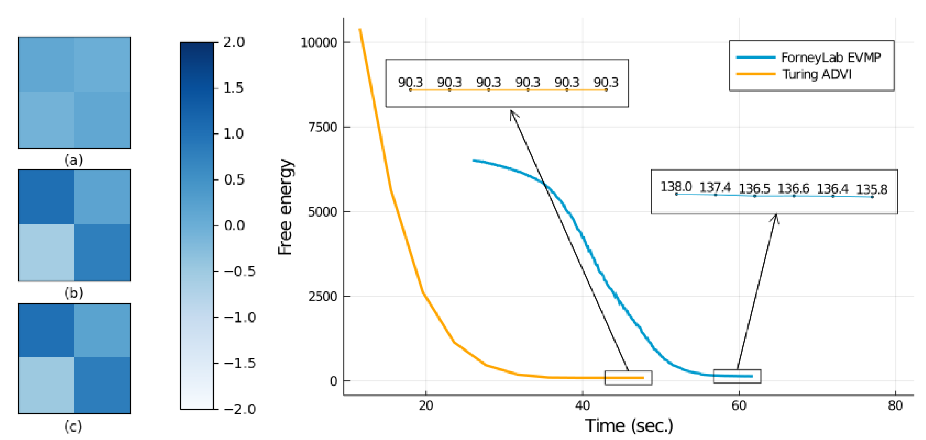
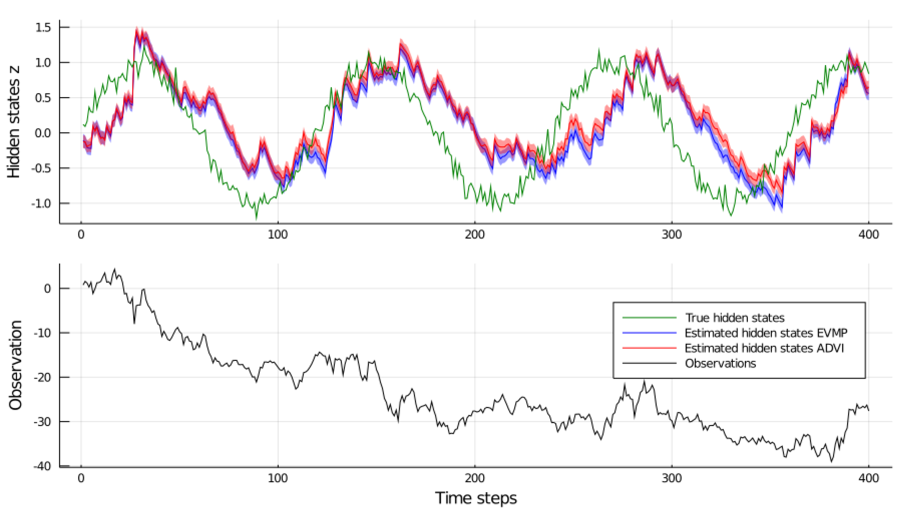
4.2. Parameter Estimation for a Linear Dynamical System

In this experiment, we focused attention on a system identification task in a Linear Dynamical System (LDS) [22,23]. An LDS is generally defined as

$$\begin{array}{cc}\hfill x_t|x_{t-1}& \sim \mathcal{N}(A{x}_{t-1},Q)\hfill \end{array}$$

(22a)

$$\begin{array}{cc}\hfill y_t|x_t& \sim \mathcal{N}(B{x}_t,R)\hfill \end{array}$$

(22b)

where $y_t$ are observations and $x_t$ are hidden states.

In this experiment, we are interested in inferring the transition matrix A together with the hidden states from a set of observations. Manually derived closed-form solutions for the system identification task are available both in maximum likelihood estimation [24] and a variational Bayesian approximation [25] contexts. Nevertheless, the goal in this and other papers on probabilistic programming packages is to automatically infer posteriors over the hidden states and parameters without resorting to manual derivations. In principle, EVMP supports to infer the hidden states, A, B, Q and R concurrently. Of course, depending on specific circumstances such as system identifiability and the richness of the observed data, the performance may vary.

In order to execute our experiment, we first extend (22a,b) with a prior on A as follows:

$$\begin{array}{cc}\hfill a& \sim \mathcal{N}({\mu }_a,V_a)\hfill \end{array}$$

(23a)

$$\begin{array}{cc}\hfill A& =\mathrm{reshape}(a,(m,m\left)\right)\hfill \end{array}$$

(23b)

$$\begin{array}{cc}\hfill x_t|x_{t-1}& \sim \mathcal{N}(A{x}_{t-1},Q)\hfill \end{array}$$

(23c)

$$\begin{array}{cc}\hfill y_t|x_t& \sim \mathcal{N}(B{x}_t,R)\hfill \end{array}$$

(23d)

In (23a–d), a holds the vectorized representation of the transition matrix A. Note that (23b) can be written as follows:

$$p\left(A\right|a)=\delta (A-\mathrm{reshape}(a,(m,m\left)\right)),$$

and through this manipulation we identify $\mathrm{reshape}(a,(m,m\left)\right)$ as the deterministic factor in (15). As a result, ForneyLab’s EVMP works out-of-the-box for inference of the transition matrix in (23a–d).

We first generated a data set of $T=40$ number of samples by running model (22a,b) with parameters $Q=0.01\times I_{2\times 2}$, $R=0.1\times I_{2\times 2}$, $B=I_{2\times 2}$ and $A=\left[\begin{array}{cc}1.0& 0.2\\ -0.5& 0.8\end{array}\right]$.

Next, we presented the data set to a second LDS model and aimed to infer posteriors over hidden states and transition matrix A. The prior on a was set to $a\sim \mathcal{N}(0_4,I_{4\times 4})$ and all other parameters were set to the same values as in the data generation process.

We compared the performance of ForneyLab’s EVMP with Turing’s ADVI and NUTS (No U-Turn Sampler, a Hamiltonian Monte Carlo sampling-based inference method) [26] engines, see Figure 5. Both EVMP, ADVI and NUTS successfully converged to almost coinciding estimates of the transition matrix (no notable difference when visualized). We also show free energy tracks for EVMP and ADVI in Figure 5. In this experiment, Turing’s ADVI outperformed ForneyLab’s EVMP in terms of total execution time and the free energy minimization. As a mitigating factor in this analysis, the pre-compilation of the message passing schedule in ForneyLab takes about 13 s, while actual execution of the generated inference algorithm is on par with Turing’s ADVI. Execution time details are shown in

Table 2. Run-time results for transition matrix estimation in the LDS model.

Algorithm	Free Energy	Total Time (s)
EVMP (ForneyLab)	135.837	$58.674\pm 0.467$
ADVI (Turing)	90.285	$47.405\pm 1.772$
NUTS (Turing)	-	$78.407\pm 4.206$

.

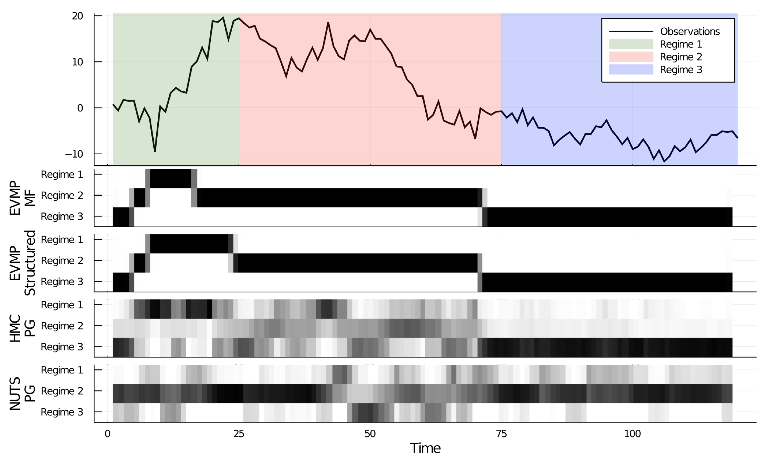
4.3. EVMP for a Switching State Space Model

In this experiment, we went beyond models that only contain continuously valued variables and inquired the capabilities of EVMP on a Switching State Space Model (SSSM) [27], which consists of both continuous and discrete hidden variables. The assumption of constant model parameters in the LDS of Section 4.2 does not account for the regime changes that occur in many dynamical systems of interest. The SSSM does allow for modeling parameter switches, and in this experiment we used the following model:

$$\begin{array}{cc}\hfill p\left(A\right)& =\prod _{k=1}^3\mathrm{Dir}(A[:,k];{\alpha }_k)\hfill \end{array}$$

(24a)

$$\begin{array}{cc}\hfill p\left(z_t\right|z_{t-1})& =\prod _{k=1}^3\prod _{j=1}^3{A}_{kj}^{z_{tk}{z}_{t-1,j}}\hfill \end{array}$$

(24b)

$$\begin{array}{cc}\hfill p\left(x_t\right|x_{t-1},z_t)& =\prod _{k=1}^3\mathcal{N}{\left(x_t\right|x_{t-1},v_k)}^{z_{tk}}\hfill \end{array}$$

(24c)

$$\begin{array}{cc}\hfill p\left(y_t\right|x_t)& =\mathcal{N}\left(y_t\right|x_t,1)\hfill \end{array}$$

(24d)

In this system, $y_t\in \mathbb{R}$ are observations, $x_t\in \mathbb{R}$ is a continuously valued hidden state and $z_t$ is a one-hot coded three-dimensional selection variable, i.e., $z_{tk}\in \{0,1\}$ and ${\sum }_{k=1}^3{z}_{tk}=1$. The parameters of the system are the state variances $v_k$ and concentration parameters ${\alpha }_k$. The elements of ${\alpha }_k$ are all 1, except the $k^{\mathrm{th}}$ element which is set to 100 to disfavor frequent regime switches, e.g., ${\alpha }_2={[1,100,1]}^{⊺}$.

We generated $T=120$ data points from a random walk process (24c) and (24d) with process noise variance parameter $v=[v_1,v_2,v_3]=[10,4,1]$. From time step $t=2$ to $t=25$, we set $z_{t,1}=1$ and consequently $p\left(x_t\right|x_{t-1})=\mathcal{N}(x_{t-1},10)$. From time step $t=26$ to $t=75$, we set $z_{t,2}=1$ and between $t=76$ to $t=T=120$ we set $z_{t,3}=1$. The generated time series is shown in Figure 6.

The main difficulty in state inference for the SSSM stems from the coupling between x and z. This is because the variational message passing rules around the node $p\left(x_t\right|x_{t-1},z_t)$ are not pre-defined in ForneyLab, although technically they can be worked out to closed-form expressions [27]. If EVMP were not available either, then a ForneyLab end user would be expected to manually derive closed-form update rules and implement these rules in an additional ForneyLab node. This type of manually assisted inference by end user calculations is what we try to avoid with EVMP and with probabilistic programming packages in general. EVMP enables the user to compensate for the lack of stored message-passing rules by introducing an auxiliary variable s in the model with a deterministic relation between s and z:

$$\begin{array}{cc}\hfill g\left(z_t\right)& =\sum _{k=1}^3{z}_{tk}·v_k\hfill \end{array}$$

(25a)

$$\begin{array}{cc}\hfill p\left(s_t\right|z_t)& =\delta (s_t-g\left(z_t\right))\hfill \end{array}$$

(25b)

$$\begin{array}{cc}\hfill p\left(x_t\right|x_{t-1},s_t)& =\mathcal{N}(x_t;x_{t-1},s_t)\hfill \end{array}$$

(25c)

$$\begin{array}{cc}\hfill p\left(x_t\right|x_{t-1},z_t)& =\int p\left(x_t\right|x_{t-1},s_t)p\left(s_t\right|z_t)\mathrm{d}{s}_t.\hfill \end{array}$$

(25d)

After we extend model specification (24a–d) by (25a–d), then ForneyLab can run EVMP-based inference out of the box. Note that there is no need for manual inference calculations, but rather a simple manipulation of the generative model that makes the system suited for automated inference.

We tested the performance of two different constraints on the posterior distribution: (1) a mean-field assumption, i.e., $q(x_{1:T},z_{1:T})={\displaystyle \prod _{t=1}^T}q\left(x_t\right)q\left(z_t\right)$; (2) a structured mean-field assumption, i.e., $q(x_{1:T},z_{1:T})=q\left(x_{1:T}\right){\displaystyle \prod _{t=1}^T}q\left(z_t\right)$, see Figure 6. We observe that the structured factorization, being a less stringent constraint on q, yields a slightly better performance than the mean-field factorization, particularly in estimating the length of the first regime.

We also compared the performance of ForneyLab’s EVMP method to Turing’s inference method. As opposed to the previous two experiments, we could not use solely ADVI, nor Hamiltonian Monte Carlo (HMC, [28,29]) and NUTS samplers in this experiment since these procedures do not allow inference for discrete random variables. Turing does provide the option to use a Particle Gibbs (PG) sampler [30,31] for the estimation of the discrete random variables ($z_{1:T}$) in conjunction with the estimation of the continuous random variables ($x_{1:T}$, A) by HMC and NUTS. The performance results for NUTS-PG and HMC-PG are shown in Figure 6. The performance of the NUTS-PG and HMC-PG samplers in estimating the correct regimes is far below the EVMP results, although the HCM-PG sampler correctly identified the third regime. The run-time scores are shown in

Table 3. Experimental results for switching state space model.

Algorithm	Free Energy	Total Time (s)
EVMP (Mean-field)	283.991	$42.722\pm 0.197$
EVMP (Structured)	273.596	$51.684\pm 0.311$
HMC-PG (Turing)	-	$116.291\pm 0.886$
NUTS-PG (Turing)	-	$51.715\pm 0.441$

.

5. Related Work

Hybrid Monte Carlo variational inference techniques have been studied prior to our work. However, mainstream research predominantly consists of variational methods within Monte Carlo techniques as opposed to our Monte Carlo methods within a variational inference approach.

For instance, ref. [32] casts variational distributions as proposal distributions in a Markov-Chain Monte Carlo (MCMC) procedure. Similarly, ref. [33] employs variational methods to design adaptive proposal distributions for Importance Sampling (IS). In [34], gradient estimates of a variational objective are used to tune the parameters of the proposal distributions for MCMC. On the other hand, Monte-Carlo Co-Ordinate Ascent Variational Inference (MC-CAVI), proposed in [35], differs from the aforementioned methods in that it uses MCMC in the calculation of expectations required within the fixed-point iterations of Coordinate Ascent Variational Inference (CAVI).

In this paper, we follow a similar approach as [35], but we use IS to estimate the expectation quantities required in VMP. Both MCMC and IS have their own merits. IS smoothly interfaces with the message passing interpretation of Bayesian inference, which further leads to automated design of proposal distributions. We use Laplace approximation for Gaussian posteriors for variables with Gaussian priors. In the context of dynamical systems, this approach notably overlaps with Gaussian filtering techniques ([36], Section 6) that is often achieved by Assumed Density Filtering ([37], Section 8.4).

As we show in Appendix E, in the approach that we propose, it is also possible to run automated Bootstrap particle filtering [36,38] rather than Gaussian filtering methods. As show in [18], particle filtering can also be framed as message passing on a factor graph. The connection between the particle filtering and variational optimization was introduced in [39]. Their formalism is based on an extension of Particle Belief Propagation [40] to Tree-Reweighted Belief Propagation [41], while ours revolves around VMP. Similar to our approach, Particle Variational Inference (PVI) [42] aims at optimizing a variational objective by successive IS approximations to true posterior distributions. While PVI applies well to inference for discrete random variables, our EVMP proposal applies to both continuous and discrete random variables.

Variational inference in the context of deterministic building blocks in probabilistic models was studied in [43]. Wheras [43] allows non-linearities to be placed only after Gaussian nodes, the proposed EVMP method generalizes this concept to EF distributed factors.

Non-conjugate Variational Message Passing (NC-VMP) [44] addresses the non-conjugate factor issue in VMP. Assuming that the posterior distribution is an EF distribution, NC-VMP projects the messages to the distribution space of the posterior by equating their sufficient statistics. Thus NC-VMP tunes the natural parameters of the messages in such a way that they converge to the stationary points of the KL divergence between the approximated and true posteriors. Ref. [44] also reports that the algorithm necessitates damping for convergence in practice. In response, ref. [45] presents Conjugate-Computation Variational Inference (CVI) as a universal inference method that is based on stochastic optimization techniques. As opposed to alternative stochastic variational inference techniques, such as Black-Box Variational Inference [46] and Automatic Differentiation Variational Inference [21], CVI exploits the conjugacy structure of the probabilistic models, which leads to faster convergence. In CVI, non-conjugate factors are incorporated into coordinate ascent steps of mean-field variational inference (with ELBO objective) through a stochastic optimization procedure to form compact posterior approximations with standard probability distributions. In our EVMP approach, the Laplace approximation entails a similarly nested optimization procedure to form compact approximations with Gaussian distributions. Nevertheless, our particle approximations to the true posteriors obviate the need for additional gradient-based optimizations to estimate the parameters of the posteriors.

Finally, the original VMP paper [9] itself briefly mentions sampling methods to overcome the issues with non-conjugate priors. However, they do not extend this idea to deterministic nodes and rather present it as a fallback method whenever soft factors are tied to non-conjugate soft factor priors. Inspired by their vision of approximating the expectation quantities by sampling techniques, we introduce here a fully automated, very broadly applicable extended VMP procedure.

6. Discussion

In this paper, we present a method for almost universal variational inference on factorized probabilistic models. The core of our method is the locality feature of VMP: the messages at a soft factor are functions of expectations related to arguments of the factor. We employ IS to estimate these expectations or directly approximate posteriors by Laplace approximation if a Gaussian posterior is reasonable. We also extended the Julia package ForneyLab with the proposed EVMP method. In contrast to many alternative PPLs that are solely based on Monte Carlo methods, ForneyLab allows end users to take full advantage of closed-form message passing rules while resorting to small-scale numerical approximations only when needed. We showed that ForneyLab provides an efficient automated variational Bayesian inference tool that in some instances may be preferable to the state-of-the-art Turing package, especially for tasks that include filtering in dynamical models or discrete variables in state space models.

While the experiments support the notion that EVMP is a promising method for inference in non-linear and non-conjugate models, we have not tested our method yet in high-dimensional problems. It is well-known that importance sampling is not efficient in high dimensions [47]. Therefore, we anticipate that for high-dimensional inference tasks with continuous random variables, Hamiltonian Monte Carlo-based methods could outperform EVMP both in terms of run-time and quality of the estimates. Nevertheless, it should be possible to alleviate the deficiencies of EVMP in high dimensions by replacing IS and Laplace approximations by HMC samplers. In essence, HMC is an MCMC method and ref. [35] shows the efficiency of MCMC methods in estimation of the expectations that are required in variational inference. Yet, in lower dimensions, we favor IS and Laplace approximations both because of their promising performance scores in the experiments and also because EVMP relieves users of choosing hyperparameters for the best performance. Recall that in the SSSM experiments in Section 4.3, we tested HMC with various hyperparameters to attain the best performance, and yet EVMP was more successful in detecting the hidden regimes. Moreover, in contrast to EVMP, plain HMC is not applicable to estimate discrete variables and needs to be combined with other samplers to run inference on the models with discrete and continuous variables.

In Appendix C, we introduce a variational free energy estimation method that resorts to approximations only if the closed-form expressions of the information-theoretic measures are not available. This differs from alternative automated variational inference techniques, such as Automatic Differentiation Variational Inference (ADVI), which estimates the entire free energy over Monte Carlo summation. Moreover, like HMC, the applicability of ADVI is also limited to continuous variables.

In EVMP, proposal distributions for importance sampling are automatically set to forward messages. Although it is a practical solution with an elegant interpretation in a message passing context, forward messages do not carry information regarding observations. Therefore, we may not acquire useful samples from forward messages if the observations lead to peaky backward messages. In future work, we aim to investigate the effects of alternative proposal distribution design methods.

One major drawback of our ForneyLab implementation is that ForneyLab does not allow loops during the inference procedure. We rarely encounter this problem with soft factors since the mean field assumption breaks the loops by imposing additional factorizations in variational distributions. However, this may not be the case with deterministic nodes. This is because the input and the output variables of deterministic nodes are tied to each other through a deterministic mapping even after the mean field assumption. For example, consider the following mixture model specification: $p\left(z\right)=\mathcal{B}er\left(\rho \right),p\left(x\right|z)=\delta (x-g_1\left(z\right))$ with $g_1\left(z\right)={\mu }_1·z+{\mu }_2·(1-z)$, $p\left(w\right|z)=\delta (w-g_2\left(z\right))$ with $g_2\left(z\right)=w_1·z+w_2·(1-z)$ and $p\left(y\right|x,w)=\mathcal{N}(x,1/w)$. Although it is a valid model specification with properly defined message passing rules, the EVMP algorithm is precluded due to the loop: the variable z is connected to two deterministic nodes ($p\left(w\right|z)$ and $p\left(x\right|z)$) the outputs of which are connected to the same node $p\left(y\right|x,w)$. Belief propagation (BP) [48,49] faces with a similar problem on loopy graphs. Nonetheless, it has been proven that iteratively running BP on loopy graphs often yields satisfactory approximations though the convergence is not guaranteed ([12], Section 8.4.7), ([37], Section 22.2). Therefore, it is worth investigating the performance of EVMP executed in a loopy setting.

There are similarities between EVMP and Expectation Propagation (EP) [50,51] in the sense that both methods estimate the moment parameters of posteriors. In contrast to EP, which approximates belief propagation (BP) [48,49] messages, EVMP approximates VMP messages, which is applicable to a broader range of model specifications. In future work, we aim to investigate and exploit this relation.

7. Conclusions

We developed a hybrid message passing-based approach to variational Bayesian inference that supports deterministic and non-conjugate model segments. The proposed Extended VMP (EVMP) method defaults to analytical updates for conjugate factor pairs and uses a local Laplace approximation or importance sampling when numerical methods are needed. EVMP was implemented in Julia’s ForneyLab package (see Appendix D) and a set of simulations shows very competitive inference performance on various inference tasks, particularly for state and parameter tracking in state-space models.

References

- van de Meent, J.W.; Paige, B.; Yang, H.; Wood, F. An Introduction to Probabilistic Programming. arXiv 2018, arXiv:1809.10756. [Google Scholar]
- Carpenter, B.; Gelman, A.; Hoffman, M.D.; Lee, D.; Goodrich, B.; Betancourt, M.; Brubaker, M.; Guo, J.; Li, P.; Riddell, A. Stan: A Probabilistic Programming Language. J. Stat. Softw. 2017, 76, 1–32. [Google Scholar] [CrossRef] [Green Version]
- Dillon, J.V.; Langmore, I.; Tran, D.; Brevdo, E.; Vasudevan, S.; Moore, D.; Patton, B.; Alemi, A.; Hoffman, M.; Saurous, R.A. TensorFlow Distributions. arXiv 2017, arXiv:1711.10604. [Google Scholar]
- Bingham, E.; Chen, J.P.; Jankowiak, M.; Obermeyer, F.; Pradhan, N.; Karaletsos, T.; Singh, R.; Szerlip, P.; Horsfall, P.; Goodman, N.D. Pyro: Deep Universal Probabilistic Programming. J. Mach. Learn. Res. 2019, 20, 1–6. [Google Scholar]
- Ge, H.; Xu, K.; Ghahramani, Z. Turing: A Language for Flexible Probabilistic Inference. In International Conference on Artificial Intelligence and Statistics; PMLR, 2018; pp. 1682–1690. [Google Scholar]
- Titsias, M.; Lázaro-Gredilla, M. Doubly stochastic variational Bayes for non-conjugate inference. In International Conference on Machine Learning; PMLR, 2014; pp. 1971–1979. [Google Scholar]
- Minka, T.; Winn, J.; Guiver, J.; Zaykov, Y.; Fabian, D.; Bronskill, J. Infer.NET 0.3. 2018. Available online: https://dotnet.github.io/infer/ (accessed on 25 June 2021).
- Cox, M.; van de Laar, T.; de Vries, B. A factor graph approach to automated design of Bayesian signal processing algorithms. Int. J. Approx. Reason. 2019, 104, 185–204. [Google Scholar] [CrossRef] [Green Version]
- Winn, J.; Bishop, C.M. Variational message passing. J. Mach. Learn. Res. 2005, 6, 661–694. [Google Scholar]
- Dauwels, J. On Variational Message Passing on Factor Graphs. In Proceedings of the IEEE International Symposium on Information Theory, Nice, France, 24–29 June 2007; pp. 2546–2550. [Google Scholar]
- Tokdar, S.T.; Kass, R.E. Importance sampling: A review. Wiley Interdiscip. Rev. Comput. Stat. 2010, 2, 54–60. [Google Scholar] [CrossRef]
- Bishop, C.M. Pattern Recognition and Machine Learning; Springer: Berlin/Heidelberg, Germany, 2006. [Google Scholar]
- Baydin, A.G.; Pearlmutter, B.A.; Radul, A.A.; Siskind, J.M. Automatic differentiation in machine learning: A survey. J. Mach. Learn. Res. 2017, 18, 5595–5637. [Google Scholar]
- Bezanson, J.; Karpinski, S.; Shah, V.B.; Edelman, A. Julia: A fast dynamic language for technical computing. arXiv 2012, arXiv:1209.5145. [Google Scholar]
- Loeliger, H.A.; Dauwels, J.; Hu, J.; Korl, S.; Ping, L.; Kschischang, F.R. The factor graph approach to model-based signal processing. Proc. IEEE 2007, 95, 1295–1322. [Google Scholar] [CrossRef] [Green Version]
- Loeliger, H.A. An introduction to factor graphs. IEEE Signal Process. Mag. 2004, 21, 28–41. [Google Scholar] [CrossRef] [Green Version]
- Blei, D.M.; Kucukelbir, A.; McAuliffe, J.D. Variational Inference: A Review for Statisticians. J. Am. Stat. Assoc. 2017, 112, 859–877. [Google Scholar] [CrossRef] [Green Version]
- Dauwels, J.; Korl, S.; Loeliger, H.A. Particle methods as message passing. In Proceedings of the IEEE International Symposium on Information Theory, Seattle, WA, USA, 9–14 July 2006; pp. 2052–2056. [Google Scholar]
- Şenöz, I.; De Vries, B. Online variational message passing in the hierarchical Gaussian filter. In Proceedings of the 2018 IEEE 28th International Workshop on Machine Learning for Signal Processing (MLSP), Aalborg, Denmark, 17–20 September 2018; pp. 1–6. [Google Scholar]
- Mathys, C.D.; Lomakina, E.I.; Daunizeau, J.; Iglesias, S.; Brodersen, K.H.; Friston, K.J.; Stephan, K.E. Uncertainty in perception and the Hierarchical Gaussian Filter. Front. Hum. Neurosci. 2014, 8, 825. [Google Scholar] [CrossRef] [Green Version]
- Kucukelbir, A.; Tran, D.; Ranganath, R.; Gelman, A.; Blei, D.M. Automatic differentiation variational inference. J. Mach. Learn. Res. 2017, 18, 430–474. [Google Scholar]
- Kalman, R.E. A new approach to linear filtering and prediction problems. J. Basic Eng. 1960, 82, 35–45. [Google Scholar] [CrossRef] [Green Version]
- Barber, D. Bayesian Reasoning and Machine Learning; Cambridge University Press: Cambridge, UK, 2012. [Google Scholar]
- Ghahramani, Z.; Hinton, G.E. Parameter Estimation for Linear Dynamical Systems; Technical Report CRG-TR-92-2; Department of Computer Science, University of Toronto: Toronto, ON, Canada, 1996. [Google Scholar]
- Beal, M.J. Variational Algorithms for Approximate Bayesian Inference. Ph.D. Thesis, UCL (University College London), London, UK, 2003. [Google Scholar]
- Hoffman, M.D.; Gelman, A. The No-U-Turn sampler: Adaptively setting path lengths in Hamiltonian Monte Carlo. J. Mach. Learn. Res. 2014, 15, 1593–1623. [Google Scholar]
- Ghahramani, Z.; Hinton, G.E. Variational learning for switching state-space models. Neural Comput. 2000, 12, 831–864. [Google Scholar] [CrossRef] [PubMed]
- Neal, R.M. MCMC using Hamiltonian dynamics. Handb. Markov Chain Monte Carlo 2011, 2, 113–162. [Google Scholar]
- Betancourt, M. A conceptual introduction to Hamiltonian Monte Carlo. arXiv 2017, arXiv:1701.02434. [Google Scholar]
- Wood, F.; Meent, J.W.; Mansinghka, V. A new approach to probabilistic programming inference. In Artificial Intelligence and Statistics; PMLR, 2014; pp. 1024–1032. [Google Scholar]
- Andrieu, C.; Doucet, A.; Holenstein, R. Particle markov chain monte carlo methods. J. R. Stat. Soc. Ser. B 2010, 72, 269–342. [Google Scholar] [CrossRef] [Green Version]
- De Freitas, N.; Højen-Sørensen, P.; Jordan, M.I.; Russell, S. Variational MCMC. In Proceedings of the Seventeenth Conference on Uncertainty in Artificial Intelligence; Morgan Kaufmann Publishers Inc.: Burlington, MA, USA, 2001; pp. 120–127. [Google Scholar]
- Wexler, Y.; Geiger, D. Importance sampling via variational optimization. In Proceedings of the Twenty-Third Conference on Uncertainty in Artificial Intelligence; AUAI Press: Arlington, VA, USA, 2007; pp. 426–433. [Google Scholar]
- Salimans, T.; Kingma, D.; Welling, M. Markov chain monte carlo and variational inference: Bridging the gap. In International Conference on Machine Learning; PMLR, 2015; pp. 1218–1226. [Google Scholar]
- Ye, L.; Beskos, A.; De Iorio, M.; Hao, J. Monte Carlo co-ordinate ascent variational inference. In Statistics and Computing; Springer: Berlin/Heidelberg, Germany, 2020; pp. 1–19. [Google Scholar]
- Särkkä, S. Bayesian Filtering and Smoothing; Cambridge University Press: Cambridge, UK, 2013; Volume 3. [Google Scholar]
- Murphy, K.P. Machine Learning: A Probabilistic Perspective; MIT Press: Cambridge, MA, USA, 2012. [Google Scholar]
- Gordon, N.J.; Salmond, D.J.; Smith, A.F. Novel approach to nonlinear/non-Gaussian Bayesian state estimation. IEEE Proc. Radar Signal Process. 1993, 140, 107–113. [Google Scholar] [CrossRef] [Green Version]
- Frank, A.; Smyth, P.; Ihler, A. Particle-based variational inference for continuous systems. Adv. Neural Inf. Process. Syst. 2009, 22, 826–834. [Google Scholar]
- Ihler, A.; McAllester, D. Particle belief propagation. In Artificial Intelligence and Statistics; PMLR, 2009; pp. 256–263. [Google Scholar]
- Wainwright, M.J.; Jaakkola, T.S.; Willsky, A.S. A new class of upper bounds on the log partition function. IEEE Trans. Inf. Theory 2005, 51, 2313–2335. [Google Scholar] [CrossRef]
- Saeedi, A.; Kulkarni, T.D.; Mansinghka, V.K.; Gershman, S.J. Variational particle approximations. J. Mach. Learn. Res. 2017, 18, 2328–2356. [Google Scholar]
- Raiko, T.; Valpola, H.; Harva, M.; Karhunen, J. Building Blocks for Variational Bayesian Learning of Latent Variable Models. J. Mach. Learn. Res. 2007, 8, 155–201. [Google Scholar]
- Knowles, D.A.; Minka, T. Non-conjugate variational message passing for multinomial and binary regression. Adv. Neural Inf. Process. Syst. 2011, 24, 1701–1709. [Google Scholar]
- Khan, M.; Lin, W. Conjugate-Computation Variational Inference: Converting Variational Inference in Non-Conjugate Models to Inferences in Conjugate Models. In Artificial Intelligence and Statistics; PMLR, 2017; pp. 878–887. [Google Scholar]
- Ranganath, R.; Gerrish, S.; Blei, D. Black box variational inference. In Artificial Intelligence and Statistics; PMLR, 2014; pp. 814–822. [Google Scholar]
- Mackay, D.J.C. Introduction to monte carlo methods. In Learning in Graphical Models; Springer: Berlin/Heidelberg, Germany, 1998; pp. 175–204. [Google Scholar]
- Pearl, J. Probabilistic Reasoning in Intelligent Systems: Networks of Plausible Inference; Morgan Kaufmann: Burlington, MA, USA, 1988. [Google Scholar]
- MacKay, D.J. Information Theory, Inference and Learning Algorithms; Cambridge University Press: Cambridge, UK, 2003. [Google Scholar]
- Minka, T.P. Expectation Propagation for approximate Bayesian inference. In Proceedings of the 17th Conference in Uncertainty in Artificial Intelligence; Morgan Kaufmann Publishers Inc.: San Francisco, CA, USA, 2001; pp. 362–369. [Google Scholar]
- Vehtari, A.; Gelman, A.; Sivula, T.; Jylänki, P.; Tran, D.; Sahai, S.; Blomstedt, P.; Cunningham, J.P.; Schiminovich, D.; Robert, C.P. Expectation Propagation as a Way of Life: A Framework for Bayesian Inference on Partitioned Data. J. Mach. Learn. Res. 2020, 21, 1–53. [Google Scholar]
- Wainwright, M.J.; Jordan, M.I. Graphical Models, Exponential Families, and Variational Inference. Found. Trends Mach. Learn. 2008, 1, 1–305. [Google Scholar] [CrossRef] [Green Version]
- Gelman, A.; Carlin, J.B.; Stern, H.S.; Dunson, D.B.; Vehtari, A.; Rubin, D.B. Bayesian Data Analysis; CRC Press: Boca Raton, FL, USA, 2013. [Google Scholar]
- Koyama, S.; Castellanos Pérez-Bolde, L.; Shalizi, C.R.; Kass, R.E. Approximate methods for state-space models. J. Am. Stat. Assoc. 2010, 105, 170–180. [Google Scholar] [CrossRef] [Green Version]
- Macke, J.H.; Buesing, L.; Cunningham, J.P.; Yu, B.M.; Shenoy, K.V.; Sahani, M. Empirical models of spiking in neural populations. Adv. Neural Inf. Process. Syst. 2011, 24, 1350–1358. [Google Scholar]
- Smola, A.J.; Vishwanathan, S.; Eskin, E. Laplace propagation. In Proceedings of the 16th International Conference on Neural Information Processing Systems; MIT Press: Cambridge, MA, USA, 2004; pp. 441–448. [Google Scholar]
- Acerbi, L. Variational bayesian monte carlo. arXiv 2018, arXiv:1810.05558. [Google Scholar]
- Ajgl, J.; Šimandl, M. Differential entropy estimation by particles. IFAC Proc. Vol. 2011, 44, 11991–11996. [Google Scholar] [CrossRef]
- Revels, J.; Lubin, M.; Papamarkou, T. Forward-Mode Automatic Differentiation in Julia. arXiv 2016, arXiv:1607.07892. [Google Scholar]
- Doucet, A.; de Freitas, N.; Gordon, N. Sequential Monte Carlo Methods in Practice; Springer: Berlin/Heidelberg, Germany, 2001. [Google Scholar]