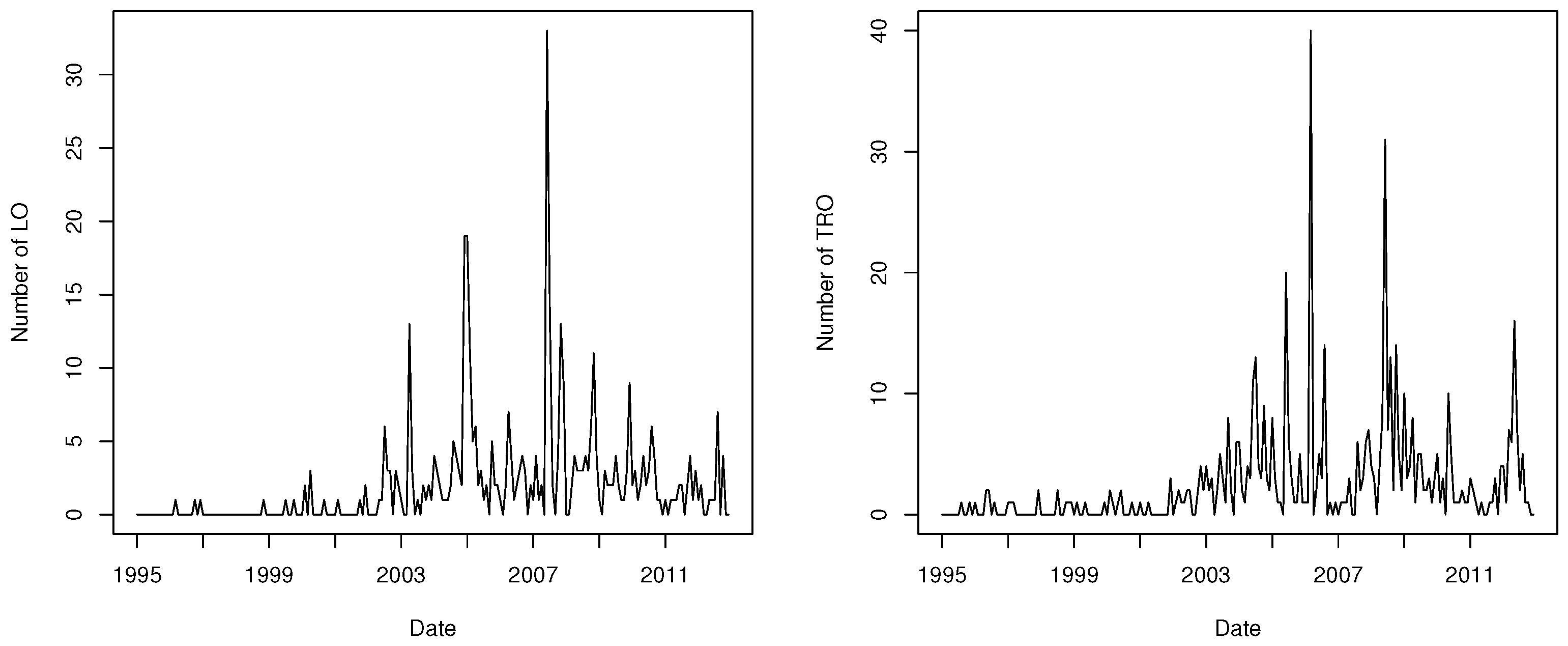
Article

Robust Estimation for Bivariate Poisson INGARCH Models

1
Department of Statistics, Yeungnam University, Gyeongsan 38541, Korea
2
Department of Statistics, Seoul National University, Seoul 08826, Korea
*
Author to whom correspondence should be addressed.
Entropy 2021, 23(3), 367; https://doi.org/10.3390/e23030367
Submission received: 15 February 2021 / Revised: 16 March 2021 / Accepted: 16 March 2021 / Published: 19 March 2021
(This article belongs to the Special Issue Time Series Modelling)

Abstract

:
In the integer-valued generalized autoregressive conditional heteroscedastic (INGARCH) models, parameter estimation is conventionally based on the conditional maximum likelihood estimator (CMLE). However, because the CMLE is sensitive to outliers, we consider a robust estimation method for bivariate Poisson INGARCH models while using the minimum density power divergence estimator. We demonstrate the proposed estimator is consistent and asymptotically normal under certain regularity conditions. Monte Carlo simulations are conducted to evaluate the performance of the estimator in the presence of outliers. Finally, a real data analysis using monthly count series of crimes in New South Wales and an artificial data example are provided as an illustration.

1. Introduction

Integer-valued time series models have received widespread attention from researchers and practitioners, due to their versatile applications in many scientific areas, including finance, insurance, marketing, and quality control. Numerous studies focus on integer-valued autoregressive (INAR) models to analyze the time series of counts, see Weiß [1] and Scotto et al. [2] for general reviews. Taking a different approach, Ferland et al. [3] proposed using Poisson integer-valued generalized autoregressive conditional heteroscedastic (INGARCH) models and Fokianos et al. [4] developed Poisson AR models to generalize the linear assumption on INGARCH models. The Poisson assumption on INGARCH models has been extended to negative binomial INGARCH models (Davis and Wu [5] and Christou and Fokianos [6]), zero-inflated generalized Poisson INGARCH models (Zhu [7,8] and Lee et al. [9]), and one-parameter exponential family AR models (Davis and Liu [10]). We refer to the review papers by Fokianos [11,12] and Tjøstheim [13,14] for more details.
Researchers invested considerable efforts to extend the univariate integer-valued time series models to bivariate (multivariate) models. For INAR type models, Quoreshi [15] proposed bivariate integer-valued moving average models and Pedeli and Karlis [16] introduced bivariate INAR models with Poisson and negative binomial innovations. Liu [17] proposed bivariate Poisson INGARCH models with a bivariate Poisson distribution that was constructed via the trivariate reduction method and established the stationarity and ergodicity of the model. Andreassen [18] later verified the consistency of the conditional maximum likelihood estimator (CMLE) and Lee et al. [19] studied the asymptotic normality of the CMLE and developed the CMLE- and residual-based change point tests. However, this model has the drawback that it can only accommodate positive correlation between two time series of counts. To cope with this issue, Cui and Zhu [20] recently introduced a new bivariate Poisson INGARCH model based on Lakshminarayana et al.’s [21] bivariate Poisson distribution. Their model can deal with positive or negative correlation, depending on the multiplicative factor parameter. They employed the CMLE for parameter estimation. However, because the CMLE is unduly influenced by outliers, the robust estimation in bivariate Poisson INGARCH models is crucial and deserves thorough investigation.
As such, here we develop a robust estimator for Cui and Zhu’s [20] bivariate Poisson INGARCH models. Among the robust estimation methods, we employ the minimum density power divergence estimator (MDPDE) approach that was originally proposed by Basu et al. [22], because it is well known to consistently provide robust estimators in various situations. For previous works in the context of time series of counts, see Kang and Lee [23], Kim and Lee [24,25], Diop and Kengne [26], Kim and Lee [27], and Lee and Kim [28], who studied the MDPDE for Poisson AR models, zero-inflated Poisson AR models, one-parameter exponential family AR models, and change point tests. For another robust estimation approach in INGARCH models, see Xiong and Zhu [29] and Li et al. [30], who studied Mallows’ quasi-likelihood method. To the best of our knowledge, the robust estimation method for bivariate Poisson INGARCH models has not been previously studied. In earlier studies, the MDPDE was proven to possess strong robust properties against outliers with little loss in asymptotic efficiency relative to the CMLE. This study confirms the same conclusion for bivariate Poisson INGARCH models.
The rest of this paper is organized, as follows. Section 2 constructs the MDPDE for bivariate Poisson INGARCH models. Section 3 shows the asymptotic properties of the MDPDE. Section 4 conducts empirical studies to evaluate the performance of the MDPDE. Section 5 provides concluding remarks. Appendix A provides the proof.

2. MDPDE for Bivariate Poisson Ingarch Models

Basu et al. [22] defined the density power divergence d α between two densities f and g, with a tuning parameter α , as
d α ( g , f ) = { f 1 + α ( y ) ( 1 + 1 α ) g ( y ) f α ( y ) + 1 α g 1 + α ( y ) } d y , α > 0 , g ( y ) ( log g ( y ) log f ( y ) ) d y , α = 0 .
For a parametric family { F θ ; θ Θ } having densities { f θ } and a distribution G with density g, they defined the minimum density power divergence functional T α ( G ) by d α ( g , f T α ( G ) ) = min θ Θ d α ( g , f θ ) . If G belongs to { F θ } , which is, G = F θ 0 for some θ 0 Θ , then T α ( F θ 0 ) = θ 0 . Let g be the density function of a random sample Y 1 , , Y n . Using the empirical distribution G n to approximate G, Basu et al. [22] defined the MDPDE by
θ ^ α , n = argmin θ Θ H α , n ( θ ) ,
where H α , n ( θ ) = 1 n t = 1 n h α , t ( θ ) and
h α , t ( θ ) = f θ 1 + α ( y ) d y 1 + 1 α f θ α ( Y t ) , α > 0 , log f θ ( Y t ) , α = 0 .
The tuning parameter α controls the trade-off between the robustness and asymptotic efficiency of the MDPDE. Namely, relatively large α values improve the robustness but the estimator’s efficiency decreases. The MDPDE with α = 0 and 1 leads to the MLE and L 2 -distance estimator, respectively. Basu et al. [22] showed the consistency and asymptotic normality of the MDPDE and demonstrated that the estimator is robust against outliers, but it still retains high efficiency when the true distribution belongs to a parametric family { F θ } and α is close to zero.
We need to define the conditional version of the MDPDE in order to apply the above procedure to bivariate Poisson INGARCH models. Let { f θ ( · | F t 1 ) } denote the parametric family of autoregressive models, being indexed by the parameter θ , and let f θ 0 ( · | F t 1 ) be the true conditional density of the time series Y t given F t 1 , where F t 1 is a σ -field generated by Y t 1 , Y t 2 , . Subsequently, the MDPDE of θ 0 is given by
θ ^ α , n = argmin θ Θ H α , n ( θ ) ,
where H α , n ( θ ) = 1 n t = 1 n h α , t ( θ ) and
h α , t ( θ ) = f θ 1 + α ( y | F t 1 ) d y 1 + 1 α f θ α ( Y t | F t 1 ) , α > 0 , log f θ ( Y t | F t 1 ) , α = 0
(cf. Section 2 of Kang and Lee [23]).
Let Y t = ( Y t , 1 , Y t , 2 ) T be a two-dimensional vector of counts at time t, namely, { Y t , 1 , t 1 } and { Y t , 2 , t 1 } are the two time series of counts under consideration. Liu [17] proposed the bivariate Poisson INGARCH model, as follows
Y t | F t 1 B P * ( λ t , 1 , λ t , 2 , ϕ ) , λ t = ( λ t , 1 , λ t , 2 ) T = ω + A λ t 1 + B Y t 1 ,
where F t is the σ -field generated by Y t , Y t 1 , , ϕ 0 , ω = ( ω 1 , ω 2 ) T R + 2 , A = { a i j } i , j = 1 , 2 and B = { b i j } i , j = 1 , 2 are 2 × 2 matrices with non-negative entries. B P * ( λ t , 1 , λ t , 2 , ϕ ) denotes the bivariate Poisson distribution constructed via the trivariate reduction method, whose probability mass function (PMF) is
P ( Y t , 1 = y 1 , Y t , 2 = y 2 | F t 1 ) = e ( λ t , 1 + λ t , 2 ϕ ) ( λ t , 1 ϕ ) y 1 y 1 ! ( λ t , 2 ϕ ) y 2 y 2 ! s = 0 min ( y 1 , y 2 ) y 1 s y 2 s s ! ϕ ( λ t , 1 ϕ ) ( λ t , 2 ϕ ) s .
In this model, C o v ( Y t , 1 , Y t , 2 | F t 1 ) = ϕ [ 0 , min ( λ t , 1 , λ t , 2 ) ) , so that the model has a drawback that it can only deal with positive correlation between two components.
To overcome this defect, Cui and Zhu [20] proposed a new bivariate Poisson INGARCH model using the distribution that was proposed by Lakshminarayana et al. [21]. They considered the model:
Y t | F t 1 B P ( λ t , 1 , λ t , 2 , δ ) , λ t = ( λ t , 1 , λ t , 2 ) T = ω + A λ t 1 + B Y t 1
and B P ( λ t , 1 , λ t , 2 , δ ) is the bivariate Poisson distribution constructed as a product of Poisson marginals with a multiplicative factor, whose PMF is given by
P ( Y t , 1 = y 1 , Y t , 2 = y 2 | F t 1 ) = λ t , 1 y 1 λ t , 2 y 2 y 1 ! y 2 ! e ( λ t , 1 + λ t , 2 ) 1 + δ ( e y 1 e c λ t , 1 ) ( e y 2 e c λ t , 2 ) ,
where c = 1 e 1 . The marginal conditional distribution of Y t , 1 and Y t , 2 are Poisson with parameters λ t , 1 and λ t , 2 , respectively, and C o v ( Y t , 1 , Y t , 2 | F t 1 ) = δ c 2 λ t , 1 λ t , 2 e c ( λ t , 1 + λ t , 2 ) . Hence, this model supports positive or negative correlation, depending on the multiplicative factor parameter δ . Cui and Zhu [20] established the stationarity and ergodicity of the model under certain conditions and showed the consistency and asymptotic normality of the CMLE.
In this study, we apply the MDPDE to the model (2). We focus on the case that A is a diagonal matrix, because this simplification can reduce the number of model parameters and makes it easy to use in practice, as Heinen and Rengifo [31] suggested. Further, the diagonal setup of A eases the verification of the asymptotic properties of the MDPDE. Similar approaches can be found in Liu [17], Lee et al. [19], and Cui et al. [32]. Let A = d i a g ( a 1 , a 2 ) . Subsequently, we set θ = ( θ 1 T , θ 2 T , δ ) T , where θ 1 = ( ω 1 , a 1 , b 11 , b 12 ) T and θ 2 = ( ω 2 , a 2 , b 21 , b 22 ) T , and write the true parameter as θ 0 = ( θ 1 0 T , θ 2 0 T , δ 0 ) T , where θ 1 0 = ( ω 1 0 , a 1 0 , b 11 0 , b 12 0 ) T and θ 2 0 = ( ω 2 0 , a 2 0 , b 21 0 , b 22 0 ) T .
Given Y 1 , , Y n that is generated from (2), from (1), we obtain the MDPDE of θ 0 by
θ ^ α , n = argmin θ Θ H ˜ α , n ( θ ) = argmin θ Θ 1 n t = 1 n h ˜ α , t ( θ ) ,
where
h ˜ α , t ( θ ) = y 1 = 0 y 2 = 0 f θ 1 + α ( y | λ ˜ t ) 1 + 1 α f θ α ( Y t | λ ˜ t ) , α > 0 , log f θ ( Y t | λ ˜ t ) , α = 0 ,
f θ ( y | λ t ) for y = ( y 1 , y 2 ) T is the conditional PMF in (3), and λ ˜ t is recursively defined by
λ ˜ t = ( λ ˜ t , 1 , λ ˜ t , 2 ) T = ω + A λ ˜ t 1 + B Y t 1 , t 2
with an arbitrarily chosen initial value λ ˜ 1 . We also use notations λ t ( θ ) and λ ˜ t ( θ ) to denote λ t and λ ˜ t , respectively, in order to emphasize the role of θ .

3. Asymptotic Properties of the MDPDE

In this section, we establish the consistency and asymptotic normality of the MDPDE. Throughout this study, A p denotes the p-induced norm of matrix A for 1 p and x p is the p-norm of vector x . When p = 1 and ∞, A 1 = max 1 j n i = 1 m | a i j | and A = max 1 i m j = 1 n | a i j | for A = { a i j } 1 i m , 1 j n , respectively. E ( · ) is taken under θ 0 . We assume that the following conditions hold in order to verify the asymptotic properties of the MDPDE.
(A1) 
θ 1 0 , θ 2 0 , and δ 0 are interior points in the compact parameter spaces Θ 1 , Θ 2 , and Θ 3 , respectively, and Θ = Θ 1 × Θ 2 × Θ 3 . In addition, there exist positive constants ω L , ω U , a L , a U , b L , b U , and δ U , such that for i , j = 1 , 2 ,
0 < ω L ω i ω U , 0 < a L a i a U , 0 < b L b i j b U , and | δ | δ U .
(A2) 
There exist positive constants φ L and φ U such that for y = ( y 1 , y 2 ) T N 0 2 , λ = ( λ 1 , λ 2 ) T ( 0 , ) 2 , and δ Θ 3 ,
0 < φ L φ ( y , λ , δ ) φ U , where φ ( y , λ , δ ) = 1 + δ ( e y 1 e c λ 1 ) ( e y 2 e c λ 2 ) .
(A3) 
There exists a p [ 1 , ] such that A p + 2 ( 1 1 / p ) B p < 1 .
Remark 1.
These conditions can be found in Cui and Zhu [20]. According to Theorem 1 in their study, { ( Y t , λ t ) } is stationary and ergodic under ( A 1 ) and ( A 3 ) .
Subsequently, we obtain the following results; the proofs are provided in the Appendix A.
Theorem 1.
Under the conditions(A1)(A3),
θ ^ α , n a . s . θ 0 a s n .
Theorem 2.
Under the conditions(A1)(A3),
n ( θ ^ α , n θ 0 ) d N ( 0 , J α 1 K α J α 1 ) a s n ,
where
J α = E 2 h α , t ( θ 0 ) θ θ T , K α = E h α , t ( θ 0 ) θ h α , t ( θ 0 ) θ T ,
and h α , t ( θ ) is defined by replacing λ ˜ t ( θ ) with λ t ( θ ) in (4).
Remark 2.
Because the tuning parameter α controls the trade-off between the robustness and asymptotic efficiency, choosing the optimal α is an important issue in practice. Several researchers investigated the selection criterion of optimal α; see Fujisawa and Eguchi [33], Durio and Isaia [34], and Toma and Broniatowski [35]. Among them, we adopt the method of Warwick [36] to choose α that minimizes the trace of the estimated asymptotic mean squared error ( A M S E ^ ) defined by
A M S E ^ = ( θ ^ α , n θ ^ 1 , n ) ( θ ^ α , n θ ^ 1 , n ) T + A s . v a r ^ ( θ ^ α , n ) ,
where θ ^ 1 , n is the MDPDE with α = 1 and A s . v a r ^ ( θ ^ α , n ) is an estimate of the asymptotic variance of θ ^ α , n , which is computed as
A s . v a r ^ ( θ ^ α , n ) = t = 1 n 2 h ˜ α , t ( θ ^ α , n ) θ θ T 1 t = 1 n h ˜ α , t ( θ ^ α , n ) θ h ˜ α , t ( θ ^ α , n ) θ T t = 1 n 2 h ˜ α , t ( θ ^ α , n ) θ θ T 1 .
This criterion is applied to our empirical study in Section 4.2.

4. Empirical Studies

4.1. Simulation

In this section, we report the simulation results to evaluate the performance of the MDPDE. The simulation settings are described, as follows. Using the inverse transformation sampling method (cf. Section 2.3 of Verges [37]), we generate Y 1 , , Y n from (2) with the initial value λ 1 = ( 0 , 0 ) T . For the estimation, λ ˜ 1 is set to be the sample mean of the data. We first consider θ = ( ω 1 , a 1 , b 11 , b 12 , ω 2 , a 2 , b 21 , b 22 , δ ) T = ( 1 , 0.2 , 0.1 , 0.2 , 0.5 , 0.3 , 0.4 , 0.2 , 0.5 ) T , which satisfies (A3) with p = 1 . In this simulation, we compare the performance of the MDPDE with α > 0 with that of the CMLE ( α = 0 ). We examine the sample mean, variance, and mean squared error (MSE) of the estimators. The sample size under consideration is n = 1000 and the number of repetitions for each simulation is 1000. In Table 1, Table 2, Table 3, Table 4, Table 5, Table 6, Table 7, Table 8, Table 9, Table 10, Table 11, Table 12, Table 13, Table 14, Table 15 and Table 16, the symbol * represents the minimal MSEs for each parameter.
Table 1 indicates that, when the data are not contaminated by outliers, the CMLE exhibits minimal MSEs for all parameters, and the MSEs of the MDPDE with small α are close to those of the CMLE. The MSE of the MDPDE shows an increasing tendency as α increases. Hence, we can conclude that the CMLE outperforms the MDPDE in the absence of outliers.
Now, we consider the situation that the data are contaminated by outliers. To this end, we generate contaminated data Y c , t = ( Y c , t , 1 , Y c , t , 2 ) T when considering
Y c , t , i = Y t , i + P t , i Y o , t , i , i = 1 , 2 ,
where Y t , i are generated from (2), P t , i are i.i.d. Bernoulli random variables with success probability p, and Y o , t , i are i.i.d. Poisson random variables with mean γ . We consider three cases: ( p , γ ) = ( 0.03 , 5 ) , ( 0.03 , 10 ) , and ( 0.05 , 10 ) . Table 2, Table 3 and Table 4 report the results. In the tables, the MDPDE appears to have smaller MSEs than the CMLE for all cases, except for the case of α = 1 when ( p , γ ) = ( 0.03 , 5 ) . As p or γ increases, the MSEs of the CMLE increase faster than those of the MDPDE, which indicates that the MDPDE outperforms the CMLE, as the data are more contaminated by outliers. Moreover, as p or γ increases, the symbol * tends to move downward. This indicates that, when the data are severely contaminated by outliers, the MDPDE with large α performs better.
We also consider smaller sample size n = 200 . The results are presented in Table 5, Table 6, Table 7 and Table 8 and they show results similar to those in Table 1, Table 2, Table 3 and Table 4. The variances and MSEs of both the CMLE and MDPDE are larger than those in Table 1, Table 2, Table 3 and Table 4.
In order to evaluate the performance of the MDPDE for negatively cross-correlated data, we consider θ = ( ω 1 , a 1 , b 11 , b 12 , ω 2 , a 2 , b 21 , b 22 , δ ) T = ( 0.5 , 0.1 , 0.2 , 0.4 , 0.3 , 0.3 , 0.2 , 0.1 , 0.4 ) T with the same p and γ , as above. The results are reported in Table 9, Table 10, Table 11, Table 12, Table 13, Table 14, Table 15 and Table 16 for n = 1000 and 200, respectively. These tables exhibit results that are similar to those in Table 1, Table 2, Table 3, Table 4, Table 5, Table 6, Table 7 and Table 8. Overall, our findings strongly support the assertion that the MDPDE is a functional tool for yielding a robust estimator for bivariate Poisson INGARCH models in the presence of outliers.

4.2. Illustrative Examples

First, we illustrate the proposed method by examining the monthly count series of crimes provided by the New South Wales Police Force in Australia. The data set is classified by local government area and offence type. This data set has been studied in many literatures, including Lee et al. [9], Chen and Lee [38,39], Kim and Lee [24], and Lee et al. [40]. To investigate the behavior of the MDPDE in the presence of outliers, we consider the data series of liquor offences (LO) and transport regulatory offences (TRO) in Botany Bay from January 1995 to December 2012, which has 216 observations in each series. Figure 1 plots the monthly count series of LO and TRO and it shows the presence of some deviant observations in each series. The sample mean and variance are 1.912 and 13.14 for LO, and 2.463 and 20.41 for TRO. A large value of the variance of each series is expected to be influenced by outliers. The autocorrelation function (ACF) and partial autocorrelation function (PACF) of LO and TRO, as well as cross-correlation function (CCF) between two series, are given in Figure 2, indicating that the data are both serially and crossly correlated. The cross-correlation coefficient between two series is 0.141.
We fit the model (2) to the data using both the CMLE and the MDPDE. λ ˜ 1 is set to be the sample mean of the data. Table 17 reports the estimated parameters with various α . The standard errors are given in parentheses and the symbol represents the minimal AMSE ^ provided in Remark 2. In the table, we can observe that the MDPDE has smaller AMSE ^ than the CMLE and the optimal α is chosen to be 0.1. The MDPDE with optimal α is quite different from the CMLE, in particular, δ ^ is about half of the CMLE. This result indicates that outliers can seriously affect the parameter estimation and, thus, the robust estimation method is required when the data are contaminated by outliers.
We clean the data by using the approach that was introduced by Fokianos and Fried [41] and apply the CMLE and the MDPDE to this data in order to illustrate the behavior of the estimators in the absence of outliers. Table 18 reports the results. The standard errors and AMSE ^ tend to decrease compared to Table 17. The CMLE has minimal AMSE ^ and the MDPDE with small α appears to be similar to the CMLE.
Now, we consider an artificial example that has negative cross-correlation coefficient. Following Cui and Zhu [20], we generate 1000 samples from univariate Poisson INGARCH model, i.e.,
X t | F t 1 P ( λ t ) , λ t = 1 + 0.35 λ t 1 + 0.45 X t 1 ,
where P ( λ t ) denotes the Poisson distribution with mean λ t . Further, we observe the contaminated data X c , t as follows
X c , t = X t + P t X o , t ,
where P t are i.i.d. Bernoulli random variables with a success probability of 0.03 and X o , t are i.i.d. Poisson random variables with mean 5. Let Y t = ( Y t , 1 , Y t , 2 ) T , where Y t , 1 = X c , t and Y t , 2 = X c , t + 500 for t = 1 , , 500 . The sample mean and variance are 5.196 and 7.380 for Y t , 1 , and 4.538 and 8.129 for Y t , 2 . The cross-correlation coefficient between Y t , 1 and Y t , 2 is −0.161. We fit the model (2) to Y t and the results are presented in Table 19. Similar to Table 17, the MDPDE has smaller AMSE ^ than the CMLE. The optimal α is chosen to be 0.3 and the corresponding δ ^ is −0.329, whereas the CMLE is 0.772.

5. Concluding Remarks

In this study, we developed the robust estimator for bivariate Poisson INGARCH models based on the MDPDE. In practice, this is important, because outliers can strongly affect the CMLE, which is commonly employed for parameter estimation in INGARCH models. We proved that the MDPDE is consistent and asymptotically normal under regularity conditions. Our simulation study compared the performances of the MDPDE and the CMLE, and confirmed the superiority of the proposed estimator in the presence of outliers. The real data analysis also confirmed the validity of our method as a robust estimator in practice. Although we focused on Cui and Zhu’s [20] bivariate Poisson INGARCH models here, the MDPDE method can be extended to other bivariate INGARCH models. For example, one can consider the copula-based bivariate INGARCH models that were studied by Heinen and Rengifo [42], Andreassen [18], and Fokianos et al. [43]. We leave this issue of extension as our future research.

Author Contributions

Conceptualization, B.K. and S.L.; methodology, B.K., S.L. and D.K.; software, B.K. and D.K.; formal analysis, B.K., S.L. and D.K.; data curation, B.K.; writing—original draft preparation, B.K. and S.L.; writing—review and editing, B.K. and S.L.; funding acquisition, B.K. and S.L. All authors have read and agreed to the published version of the manuscript.

Funding

This work was supported by the National Research Foundation of Korea (NRF) grant funded by the Korea government (MSIT), grant no. NRF-2019R1C1C1004662 (B.K.) and 2021R1A2C1004009 (S.L.).

Data Availability Statement

Publicly available datasets were analyzed in this study. This data can be found here: data.gov.au (accessed on 19 March 2021).

Conflicts of Interest

The authors declare no conflict of interest.

Appendix A

In this Appendix, we provide the proofs for Theorems 1 and 2 in Section 3 when α > 0 . We refer to Cui and Zhu [20] for the case of α = 0 . In what follows, we denote V and ρ ( 0 , 1 ) as a generic positive integrable random variable and a generic constant, respectively, and H α , n ( θ ) = n 1 t = 1 n h α , t ( θ ) . Furthermore, we employ the notation λ t = λ t ( θ ) , λ ˜ t = λ ˜ t ( θ ) , λ t 0 = λ t ( θ 0 ) , λ t , i = λ t , i ( θ i ) , λ ˜ t , i = λ ˜ t , i ( θ i ) , λ t , i 0 = λ t , i ( θ i 0 ) for i = 1 , 2 , and u ( y , λ ) = e y e c λ for brevity.
Lemma A1.
Under(A1)(A3), we have for i = 1 , 2 ,
(i) 
E ( sup θ i Θ i λ t , i ) < .
(ii) 
λ t , i = λ t , i 0 a.s. implies θ i = θ i 0 .
(iii) 
λ t , i is twice continuously differentiable with respect to θ i and satisfies
E sup θ i Θ i λ t , i θ i 1 4 < a n d E sup θ i Θ i 2 λ t , i θ i θ i T 1 2 < .
(iv) 
sup θ i Θ i λ t , i θ i λ ˜ t , i θ i 1 V ρ t a . s .
(v) 
ν T λ t , i 0 θ i = 0 a.s. implies ν = 0 .
(vi) 
sup θ i Θ i | λ t , i λ ˜ t , i | V ρ t a.s.
Proof. 
By recursion of (2), we have
λ t = ( I 2 A ) 1 ω + k = 0 A k B Y t k 1 , λ ˜ t = ( I 2 + A + + A t 2 ) ω + A t 1 λ ˜ 1 + k = 0 t 2 A k B Y t k 1
and thus, for i = 1 , 2 ,
λ t , i = ω i 1 a i + k = 0 a i k ( b i 1 Y t k 1 , 1 + b i 2 Y t k 1 , 2 ) , λ ˜ t , i = ω i 1 a i + k = 0 t 2 a i k ( b i 1 Y t k 1 , 1 + b i 2 Y t k 1 , 2 ) ,
where I 2 denotes 2 × 2 identity matrix and the initial value λ ˜ 1 , i is taken as ω i / ( 1 a i ) for simplicity. Subsequently, ( i ) ( v ) can be shown following the arguments in the proof of Theorem 3 in Kang and Lee [44]. For ( v i ) , let ρ = sup θ i Θ i a i < 1 . Afterwards, from (2), it holds that
sup θ i Θ i | λ t , i λ ˜ t , i | = sup θ i Θ i | a i ( λ t 1 , i λ ˜ t 1 , i ) | = = sup θ i Θ i | a i t 1 ( λ 1 , i λ ˜ 1 , i ) | V ρ t
with V = sup θ i Θ i | λ 1 , i λ ˜ 1 , i | / ρ . Therefore, the lemma is established. □
Lemma A2.
Under(A1)(A3), we have
sup θ Θ | H α , n ( θ ) H ˜ α , n ( θ ) | a . s . 0 a s n .
Proof. 
It is sufficient to show that
sup θ Θ | h α , t ( θ ) h ˜ α , t ( θ ) | a . s . 0 a s t .
We write
| h α , t ( θ ) h ˜ α , t ( θ ) | y 1 = 0 y 2 = 0 f θ 1 + α ( y | λ t ) f θ 1 + α ( y | λ ˜ t ) + 1 + 1 α f θ α ( Y t | λ t ) f θ α ( Y t | λ ˜ t ) : = I t ( θ ) + I I t ( θ ) .
From ( A 1 ) , ( A 2 ) , and the mean value theorem (MVT), we have
I t ( θ ) = ( 1 + α ) y 1 = 0 y 2 = 0 f θ 1 + α ( y | λ t * ) y 1 λ t , 1 * 1 + c δ e c λ t , 1 * u ( y 2 , λ t , 2 * ) φ ( y , λ t * , δ ) ( λ t , 1 λ ˜ t , 1 ) + y 1 = 0 y 2 = 0 f θ 1 + α ( y | λ t * ) y 2 λ t , 2 * 1 + c δ e c λ t , 2 * u ( y 1 , λ t , 1 * ) φ ( y , λ t * , δ ) ( λ t , 2 λ ˜ t , 2 ) ( 1 + α ) y 1 = 0 y 2 = 0 f θ ( y | λ t * ) y 1 λ t , 1 * + 1 + c | δ | e c λ t , 1 * | u ( y 2 , λ t , 2 * ) | φ ( y , λ t * , δ ) | λ t , 1 λ ˜ t , 1 | + y 1 = 0 y 2 = 0 f θ ( y | λ t * ) y 2 λ t , 2 * + 1 + c | δ | e c λ t , 2 * | u ( y 1 , λ t , 1 * ) | φ ( y , λ t * , δ ) | λ t , 2 λ ˜ t , 2 | ( 1 + α ) 1 + 1 + 2 c δ U φ L | λ t , 1 λ ˜ t , 1 | + 1 + 1 + 2 c δ U φ L | λ t , 2 λ ˜ t , 2 | = 2 ( 1 + α ) 1 + c δ U φ L ( | λ t , 1 λ ˜ t , 1 | + | λ t , 2 λ ˜ t , 2 | ) ,
where λ t * = ( λ t , 1 * , λ t , 2 * ) T and λ t , i * is an intermediate point between λ t , i and λ ˜ t , i for i = 1 , 2 . Hence, sup θ Θ I t ( θ ) converges to 0 a.s. as t by ( v i ) of Lemma A1.
Because λ t , i * = m λ t , i + ( 1 m ) λ ˜ t , i for some m ( 0 , 1 ) , it holds that ( λ t , i * ) 1 ( m λ t , i ) 1 ( m ω L ) 1 . Thus, we obtain
I I t ( θ ) = ( 1 + α ) f θ α ( Y t | λ t * ) Y t , 1 λ t , 1 * 1 + c δ e c λ t , 1 * u ( Y t , 2 , λ t , 2 * ) φ ( Y t , λ t * , δ ) ( λ t , 1 λ ˜ t , 1 ) + f θ α ( Y t | λ t * ) Y t , 2 λ t , 2 * 1 + c δ e c λ t , 2 * u ( Y t , 1 , λ t , 1 * ) φ ( Y t , λ t * , δ ) ( λ t , 2 λ ˜ t , 2 ) ( 1 + α ) Y t , 1 m ω L + 1 + 2 c δ U φ L | λ t , 1 λ ˜ t , 1 | + Y t , 2 m ω L + 1 + 2 c δ U φ L | λ t , 2 λ ˜ t , 2 | .
According to Lemma 2.1 in Straumann and Mikosch [45], together with ( v i ) of Lemma A1, sup θ Θ I I t ( θ ) converges to 0 a.s. as t . Therefore, the lemma is verified. □
Lemma A3.
Under(A1)(A3), we have
E sup θ Θ | h α , t ( θ ) | < a n d   i f θ θ 0 , t h e n E ( h α , t ( θ ) ) > E ( h α , t ( θ 0 ) ) .
Proof. 
Because
| h α , t ( θ ) | y 1 = 0 y 2 = 0 f θ 1 + α ( y | λ t ) + 1 + 1 α f θ α ( Y t | λ t ) 2 + 1 α ,
the first part of the lemma is validated. Note that
E ( h α , t ( θ ) ) E ( h α , t ( θ 0 ) ) = E E h α , t ( θ ) h α , t ( θ 0 ) | F t 1 = E y 1 = 0 y 2 = 0 f θ 1 + α ( y | λ t ) 1 + 1 α f θ α ( y | λ t ) f θ 0 ( y | λ t ) + 1 α f θ 0 1 + α ( y | λ t ) 0 ,
where the equality holds if and only if δ = δ 0 and λ t = λ t 0 a.s. Therefore, the second part of the lemma is established by ( i i ) of Lemma A1. □
Proof of Theorem 1. 
We can write
sup θ Θ 1 n t = 1 n h ˜ α , t ( θ ) E ( h α , t ( θ ) ) sup θ Θ 1 n t = 1 n h ˜ α , t ( θ ) 1 n t = 1 n h α , t ( θ ) + sup θ Θ 1 n t = 1 n h α , t ( θ ) E ( h α , t ( θ ) ) .
The first term on the RHS of the inequality converges to 0 a.s. from Lemma A2. Moreover, because h α , t ( θ ) is stationary and ergodic with E ( sup θ Θ | h α , t ( θ ) | ) < by Lemma A3, the second term also converges to 0 a.s. Finally, as E ( h α , t ( θ ) ) has a unique minimum at θ 0 from Lemma A3, the theorem is established. □
Now, we derive the first and second derivatives of h α , t ( θ ) . The first derivatives are obtained as
h α , t ( θ ) θ = ( 1 + α ) D t , 1 ( θ ) s t , 1 ( θ 1 ) T , D t , 2 ( θ ) s t , 2 ( θ 2 ) T , D t , 3 ( θ ) T = ( 1 + α ) D t , 1 ( θ ) I 4 0 4 × 4 0 4 × 1 0 4 × 4 D t , 2 ( θ ) I 4 0 4 × 1 0 1 × 4 0 1 × 4 D t , 3 ( θ ) s t , 1 ( θ 1 ) s t , 2 ( θ 2 ) 1 : = ( 1 + α ) D t ( θ ) Λ t ( θ ) ,
where I 4 denotes the 4 × 4 identity matrix, 0 m × n means the m × n matrix with zero elements, and
s t , i ( θ i ) = λ t , i θ i for i = 1 , 2 , D t , i ( θ ) = y 1 = 0 y 2 = 0 f θ 1 + α ( y | λ t ) y i λ t , i 1 + c δ e c λ t , i u ( y j , λ t , j ) φ ( y , λ t , δ ) f θ α ( Y t | λ t ) Y t , i λ t , i 1 + c δ e c λ t , i u ( Y t , j , λ t , j ) φ ( Y t , λ t , δ ) for ( i , j ) = ( 1 , 2 ) , ( 2 , 1 ) , D t , 3 ( θ ) = y 1 = 0 y 2 = 0 f θ 1 + α ( y | λ t ) u ( y 1 , λ t , 1 ) u ( y 2 , λ t , 2 ) φ ( y , λ t , δ ) f θ α ( Y t | λ t ) u ( Y t , 1 , λ t , 1 ) u ( Y t , 2 , λ t , 2 ) φ ( Y t , λ t , δ ) .
The second derivatives are expressed as
2 h α , t ( θ ) θ θ T = ( 1 + α ) F t , 11 ( θ ) s t , 1 ( θ 1 ) s t , 1 ( θ 1 ) T F t , 12 ( θ ) s t , 1 ( θ 1 ) s t , 2 ( θ 2 ) T F t , 13 ( θ ) s t , 1 ( θ 1 ) F t , 21 ( θ ) s t , 2 ( θ 2 ) s t , 1 ( θ 1 ) T F t , 22 ( θ ) s t , 2 ( θ 2 ) s t , 2 ( θ 2 ) T F t , 23 ( θ ) s t , 2 ( θ 2 ) F t , 31 ( θ ) s t , 1 ( θ 1 ) T F t , 32 ( θ ) s t , 2 ( θ 2 ) T F t , 33 ( θ ) + ( 1 + α ) D t , 1 ( θ ) s t , 11 ( θ 1 ) 0 4 × 4 0 4 × 1 0 4 × 4 D t , 2 ( θ ) s t , 22 ( θ 2 ) 0 4 × 1 0 1 × 4 0 1 × 4 0 : = ( 1 + α ) F t ( θ ) + D t ( θ ) Λ t ( θ ) θ T ,
where
s t , i i ( θ i ) = 2 λ t , i θ i θ i T for i = 1 , 2 , F t , i i ( θ ) = y 1 = 0 y 2 = 0 f θ 1 + α ( y | λ t ) ( 1 + α ) y i λ t , i 1 + c δ e c λ t , i u ( y j , λ t , j ) φ ( y , λ t , δ ) 2 y i λ t , i 2 c 2 δ e c λ t , i u ( y j , λ t , j ) 1 + δ e y i u ( y j , λ t , j ) φ ( y , λ t , δ ) 2 f θ α ( Y t | λ t ) α Y t , i λ t , i 1 + c δ e c λ t , i u ( Y t , j , λ t , j ) φ ( Y t , λ t , δ ) 2 Y t , i λ t , i 2 c 2 δ e c λ t , i u ( Y t , j , λ t , j ) 1 + δ e Y t , i u ( Y t , j , λ t , j ) φ ( Y t , λ t , δ ) 2 for ( i , j ) = ( 1 , 2 ) , ( 2 , 1 ) , F t , 33 ( θ ) = α y 1 = 0 y 2 = 0 f θ 1 + α ( y | λ t ) u ( y 1 , λ t , 1 ) u ( y 2 , λ t , 2 ) φ ( y , λ t , δ ) 2 ( α 1 ) f θ α ( Y t | λ t ) u ( Y t , 1 , λ t , 1 ) u ( Y t , 2 , λ t , 2 ) φ ( Y t , λ t , δ ) 2 , F t , 12 ( θ ) = y 1 = 0 y 2 = 0 f θ 1 + α ( y | λ t ) ( 1 + α ) y 1 λ t , 1 1 + c δ e c λ t , 1 u ( y 2 , λ t , 2 ) φ ( y , λ t , δ ) × y 2 λ t , 2 1 + c δ e c λ t , 2 u ( y 1 , λ t , 1 ) φ ( y , λ t , δ ) + c 2 δ e c ( λ t , 1 + λ t , 2 ) φ ( y , λ t , δ ) 2 f θ α ( Y t | λ t ) α Y t , 1 λ t , 1 1 + c δ e c λ t , 1 u ( Y t , 2 , λ t , 2 ) φ ( Y t , λ t , δ ) × Y t , 2 λ t , 2 1 + c δ e c λ t , 2 u ( Y t , 1 , λ t , 1 ) φ ( Y t , λ t , δ ) + c 2 δ e c ( λ t , 1 + λ t , 2 ) φ ( Y t , λ t , δ ) 2 , F t , i 3 ( θ ) = y 1 = 0 y 2 = 0 f θ 1 + α ( y | λ t ) ( 1 + α ) y i λ t , i 1 + c δ e c λ t , i u ( y j , λ t , j ) φ ( y , λ t , δ ) × u ( y 1 , λ t , 1 ) u ( y 2 , λ t , 2 ) φ ( y , λ t , δ ) + c e c λ t , i u ( y j , λ t , j ) φ ( y , λ t , δ ) 2 f θ α ( Y t | λ t ) α Y t , i λ t , i 1 + c δ e c λ t , i u ( Y t , j , λ t , j ) φ ( Y t , λ t , δ ) u ( Y t , 1 , λ t , 1 ) u ( Y t , 2 , λ t , 2 ) φ ( Y t , λ t , δ ) + c e c λ t , i u ( Y t , j , λ t , j ) φ ( Y t , λ t , δ ) 2 for ( i , j ) = ( 1 , 2 ) , ( 2 , 1 ) .
The following four lemmas are helpful for proving Theorem 2.
Lemma A4.
Let D ˜ t , i ( θ ) denote the counterpart of D t , i ( θ ) by substituting λ t with λ ˜ t for i = 1 , 2 , 3 . Subsequently, under(A1)(A3), we have that for i = 1 , 2 ,
| D t , i ( θ ) | C ( Y t , i + 1 ) , | D ˜ t , i ( θ ) | C ( Y t , i + 1 ) , | D t , 3 ( θ ) | C , | D ˜ t , 3 ( θ ) | C , | F t , i i ( θ ) | C ( Y t , i 2 + Y t , i + 1 ) , | F t , 33 ( θ ) | C , | F t , 12 ( θ ) | C ( Y t , 1 Y t , 2 + Y t , 1 + Y t , 2 + 1 ) , | F t , i 3 ( θ ) | C ( Y t , i + 1 ) ,
and for ( i , j ) = ( 1 , 2 ) , ( 2 , 1 ) ,
| D t , i ( θ ) D ˜ t , i ( θ ) | C ( Y t , i 2 + Y t , i + 1 ) | λ t , i λ ˜ t , i | + C ( Y t , 1 Y t , 2 + Y t , 1 + Y t , 2 + 1 ) | λ t , j λ ˜ t , j | , | D t , 3 ( θ ) D ˜ t , 3 ( θ ) | C ( Y t , 1 + 1 ) | λ t , 1 λ ˜ t , 1 | + C ( Y t , 2 + 1 ) | λ t , 2 λ ˜ t , 2 | ,
where C is some positive constant.
Proof. 
From (A1)(A3) and the fact that λ t , i 1 ω L 1 , we obtain
| D t , i ( θ ) | y 1 = 0 y 2 = 0 f θ ( y | λ t ) y i λ t , i + 1 + c | δ | e c λ t , i | u ( y j , λ t , j ) | φ ( y , λ t , δ ) + Y t , i λ t , i + 1 + c | δ | e c λ t , i | u ( Y t , j , λ t , j ) | φ ( Y t , λ t , δ ) 1 + 1 + 2 c δ U φ L + Y t , i ω L + 1 + 2 c δ U φ L = Y t , i ω L + 3 + 4 c δ U φ L
for ( i , j ) = ( 1 , 2 ) , ( 2 , 1 ) and
| D t , 3 ( θ ) | y 1 = 0 y 2 = 0 f θ ( y | λ t ) | u ( y 1 , λ t , 1 ) | | u ( y 2 , λ t , 2 ) | φ ( y , λ t , δ ) + | u ( Y t , 1 , λ t , 1 ) | | u ( Y t , 2 , λ t , 2 ) | φ ( Y t , λ t , δ ) = 8 φ L .
The second and fourth parts of the lemma also hold in the same manner. Furthermore, we can show that
| F t , i i ( θ ) | y 1 = 0 y 2 = 0 f θ ( y | λ t ) 2 ( 1 + α ) y i λ t , i λ t , i 2 + c δ e c λ t , i u ( y j , λ t , j ) φ ( y , λ t , δ ) 2 + y i λ t , i 2 + c 2 | δ | e c λ t , i | u ( y j , λ t , j ) | 1 + | δ | e y i | u ( y j , λ t , j ) | φ ( y , λ t , δ ) 2 + 2 α Y t , i λ t , i 1 2 + c δ e c λ t , i u ( Y t , j , λ t , j ) φ ( Y t , λ t , δ ) 2 Y t , i λ t , i 2 c 2 | δ | e c λ t , i | u ( Y t , j , λ t , j ) | 1 + | δ | e Y t , i | u ( Y t , j , λ t , j ) | φ ( Y t , λ t , δ ) 2 2 ( 1 + α ) 1 ω L + 2 ( 1 + α ) 4 c 2 δ U 2 φ L 2 + 1 ω L + 2 c 2 δ U ( 1 + 2 δ U ) φ L 2 + 4 α Y t , i 2 ω L 2 + 4 α + 2 α 4 c 2 δ U 2 φ L 2 + Y t , i ω L 2 + 2 c 2 δ U ( 1 + 2 δ U ) φ L 2 = 4 α ω L 2 Y t , i 2 + 1 ω L 2 Y t , i + 3 + 2 α ω L + 4 c 2 δ U 4 ( 1 + α ) δ U + 1 φ L 2 + 4 α
for ( i , j ) = ( 1 , 2 ) , ( 2 , 1 ) ,
| F t , 33 ( θ ) | α y 1 = 0 y 2 = 0 f θ ( y | λ t ) u ( y 1 , λ t , 1 ) u ( y 2 , λ t , 2 ) φ ( y , λ t , δ ) 2 + ( 1 + α ) u ( Y t , 1 , λ t , 1 ) u ( Y t , 2 , λ t , 2 ) φ ( Y t , λ t , δ ) 2 16 α φ L 2 + 16 ( 1 + α ) φ L 2 = 16 ( 1 + 2 α ) φ L 2 ,
| F t , 12 ( θ ) | y 1 = 0 y 2 = 0 f θ ( y | λ t ) ( 1 + α ) y 1 λ t , 1 + 1 + c | δ | e c λ t , 1 | u ( y 2 , λ t , 2 ) | φ ( y , λ t , δ ) × y 2 λ t , 2 + 1 + c | δ | e c λ t , 2 | u ( y 1 , λ t , 1 ) | φ ( y , λ t , δ ) + c 2 | δ | e c ( λ t , 1 + λ t , 2 ) φ ( y , λ t , δ ) 2 + α Y t , 1 λ t , 1 + 1 + c | δ | e c λ t , 1 | u ( Y t , 2 , λ t , 2 ) | φ ( Y t , λ t , δ ) × Y t , 2 λ t , 2 + 1 + c | δ | e c λ t , 2 | u ( Y t , 1 , λ t , 1 ) | φ ( Y t , λ t , δ ) + c 2 | δ | e c ( λ t , 1 + λ t , 2 ) φ ( Y t , λ t , δ ) 2 ( 1 + α ) c 2 δ U + 1 + 1 + 2 c δ U φ L + 1 + 2 c δ U φ L + 4 c 2 δ U 2 φ L 2 + 4 c δ U φ L + 1 + c 2 δ U φ L 2 + α Y t , 1 Y t , 2 ω L 2 + 1 ω L 1 + 2 c δ U φ L ( Y t , 1 + Y t , 2 ) + 4 c 2 δ U 2 φ L 2 + 4 c δ U φ L + 1 + c 2 δ U φ L 2 = α ω L 2 Y t , 1 Y t , 2 + α ω L 1 + 2 c δ U φ L ( Y t , 1 + Y t , 2 ) + 4 ( 1 + 2 α ) c 2 δ U 2 φ L 2 + 2 c 2 δ U φ L 2 + 4 ( 2 + 3 α ) c δ U φ L + ( 1 + α ) c 2 δ U + 4 + 5 α ,
and
| F t , i 3 ( θ ) | y 1 = 0 y 2 = 0 f θ ( y | λ t ) ( 1 + α ) y i λ t , i + 1 + c | δ | e c λ t , i | u ( y j , λ t , j ) | φ ( y , λ t , δ ) × | u ( y 1 , λ t , 1 ) | | u ( y 2 , λ t , 2 ) | φ ( y , λ t , δ ) + c e c λ t , i | u ( y j , λ t , j ) | φ ( y , λ t , δ ) 2 + α Y t , i λ t , i + 1 + c | δ | e c λ t , i | u ( Y t , j , λ t , j ) | φ ( Y t , λ t , δ ) | u ( Y t , 1 , λ t , 1 ) | | u ( Y t , 2 , λ t , 2 ) | φ ( Y t , λ t , δ ) + c e c λ t , i | u ( Y t , j , λ t , j ) | φ ( Y t , λ t , δ ) 2 4 ( 1 + α ) φ L 1 + 1 + 2 c δ U φ L + 2 c φ L 2 + 4 α φ L Y t , i ω L + 1 + 2 c δ U φ L + 2 c φ L 2 = 4 α φ L ω L Y t , i + 4 c { 1 + 2 ( 1 + 2 α ) δ U } φ L 2 + 4 ( 2 + 3 α ) φ L
for ( i , j ) = ( 1 , 2 ) , ( 2 , 1 ) .
Now, we prove the last two parts of the lemma. Because F t , i j ( θ ) = D t , i ( θ ) / λ t , j for i = 1 , 2 , 3 , j = 1 , 2 , owing to MVT, it holds that for i = 1 , 2 , 3 ,
| D t , i ( θ ) D ˜ t , i ( θ ) | D t , i ( θ ) λ t , 1 | λ t = λ t * | λ t , 1 λ ˜ t , 1 | + D t , i ( θ ) λ t , 2 | λ t = λ t * | λ t , 2 λ ˜ t , 2 | = F t , i 1 ( θ ) | λ t = λ t * | λ t , 1 λ ˜ t , 1 | + F t , i 2 ( θ ) | λ t = λ t * | λ t , 2 λ ˜ t , 2 | ,
where F t , i j ( θ ) | λ t = λ t * is the same as F t , i j ( θ ) with λ t replaced by λ t * for j = 1 , 2 . Because ( λ t , i * ) 1 ω L 1 , it can be easily shown that F t , i j ( θ ) | λ t = λ t * has the same upper bound as F t , i j ( θ ) by following the aforementioned arguments. Therefore, the lemma is established. □
Lemma A5.
Under(A1)(A3), we have
E sup θ Θ 2 h α , t ( θ ) θ θ T 1 < a n d E sup θ Θ h α , t ( θ ) θ h α , t ( θ ) θ T 1 < .
Proof. 
We can write
E sup θ Θ 2 h α , t ( θ ) θ θ T 1 ( 1 + α ) E sup θ Θ F t ( θ ) 1 + E sup θ Θ D t ( θ ) Λ t ( θ ) θ T 1 .
Hence, to show the first part of the lemma, it is sufficient to show that, for i , j = 1 , 2 ,
E sup θ Θ F t , i j ( θ ) λ t , i θ i λ t , j θ j T 1 < , E sup θ Θ F t , i 3 ( θ ) λ t , i θ i 1 < , E sup θ Θ | F t , 33 ( θ ) | < , and E sup θ Θ D t , i ( θ ) 2 λ t , i θ i θ i T 1 < ,
which can be directly obtained from ( i i i ) of Lemma A1, Lemma A4, and Cauchy–Schwarz inequality. For example,
E sup θ Θ F t , 12 ( θ ) λ t , 1 θ 1 λ t , 2 θ 2 T 1 E sup θ Θ | F t , 12 ( θ ) | 2 1 / 2 E sup θ Θ λ t , 1 θ 1 λ t , 2 θ 2 T 1 2 1 / 2 E C ( Y t , 1 Y t , 2 + Y t , 1 + Y t , 2 + 1 ) 2 1 / 2 × E sup θ 1 Θ 1 λ t , 1 θ 1 1 4 1 / 4 E sup θ 2 Θ 2 λ t , 2 θ 2 1 4 1 / 4 <
and
E sup θ Θ D t , 1 ( θ ) 2 λ t , 1 θ 1 θ 1 T 1 E sup θ Θ | D t , 1 ( θ ) | 2 1 / 2 E sup θ 1 Θ 1 2 λ t , 1 θ 1 θ 1 T 1 2 1 / 2 E C ( Y t , 1 + 1 ) 2 1 / 2 E sup θ 1 Θ 1 2 λ t , 1 θ 1 θ 1 T 1 2 1 / 2 < .
The second part of the lemma can be shown in the same manner. □
Lemma A6.
Under(A1)(A3), we have
1 n t = 1 n sup θ Θ h α , t ( θ ) θ h ˜ α , t ( θ ) θ 1 a . s . 0 a s n .
Proof. 
Owing to ( i v ) and ( v i ) of Lemma A1 and Lemma A4, we obtain a.s.,
1 1 + α sup θ Θ h α , t ( θ ) θ h ˜ α , t ( θ ) θ 1 sup θ Θ D ˜ t ( θ ) 1 sup θ Θ Λ t ( θ ) Λ ˜ t ( θ ) 1 + sup θ Θ Λ t ( θ ) 1 sup θ Θ D t ( θ ) D ˜ t ( θ ) 1 i = 1 3 sup θ Θ | D ˜ t , i ( θ ) | i = 1 2 sup θ i Θ i λ t , i θ i λ ˜ t , i θ i 1 + i = 1 2 sup θ i Θ i λ t , i θ i 1 + 1 i = 1 3 sup θ Θ | D t , i ( θ ) D ˜ t , i ( θ ) | 2 C ( Y t , 1 + Y t , 2 + 3 ) V ρ t + i = 1 2 sup θ i Θ i λ t , i θ i 1 + 1 × C Y t , 1 2 + Y t , 2 2 + 2 Y t , 1 Y t , 2 + 4 ( Y t , 1 + Y t , 2 ) + 6 V ρ t ,
where D ˜ t ( θ ) and Λ ˜ t ( θ ) are the same as D t ( θ ) and Λ t ( θ ) with λ t replaced by λ ˜ t . Therefore, from Lemma 2.1 in Straumann and Mikosch [45], together with ( i i i ) of Lemma A1, the RHS of the last inequality converges to 0 exponentially fast a.s. and, thus, the lemma is validated. We refer the reader to Straumann and Mikosch [45] and Cui and Zheng [46] for more details on exponentially fast a.s. convergence. □
Lemma A7.
Let θ ^ α , n H = argmin θ Θ H α , n ( θ ) . Subsequently, under(A1)(A3), we have
θ ^ α , n H a . s . θ 0 a n d n ( θ ^ α , n H θ 0 ) d N ( 0 , J α 1 K α J α 1 ) a s n .
Proof. 
As seen in the proof of Theorem 1, sup θ Θ n 1 t = 1 n h α , t ( θ ) E ( h α , t ( θ ) ) converges to 0 a.s. and E ( h α , t ( θ ) ) has a unique minimum at θ 0 . Hence, the first part of the lemma is verified.
Next, we handle the second part. Let θ ( i ) , i = 1 , , 9 be the i-th element of θ . Using MVT, we have
0 = 1 n t = 1 n h α , t ( θ 0 ) θ ( i ) + n ( θ ^ α , n H θ 0 ) T 1 n t = 1 n 2 h α , t ( θ α , n , i * ) θ θ ( i )
for some vector θ α , n , i * between θ 0 and θ ^ α , n H , so that, eventually, we can write
0 = 1 n t = 1 n h α , t ( θ 0 ) θ + n ( θ ^ α , n H θ 0 ) T 1 n t = 1 n 2 h α , t ( θ α , n * ) θ θ T ,
where the term 2 h α , t ( θ α , n * ) / θ θ T actually represents a 9 × 9 matrix whose ( i , j ) -th entry is 2 h α , t ( θ α , n , i j * ) / θ ( i ) θ ( j ) for some vector θ α , n , i j * between θ 0 and θ ^ α , n H . We first show that
1 n t = 1 n h α , t ( θ 0 ) θ d N ( 0 , K α ) .
For ν = ( ν 1 T , ν 2 T , ν 3 ) T R 4 × R 4 × R , we obtain
E ν T h α , t ( θ 0 ) θ | F t 1 = ( 1 + α ) ν 1 T λ t , 1 0 θ 1 E D t , 1 ( θ 0 ) | F t 1 + ν 2 T λ t , 2 0 θ 2 E D t , 2 ( θ 0 ) | F t 1 + ν 3 E D t , 3 ( θ 0 ) | F t 1 = 0
and
E ν T h α , t ( θ 0 ) θ 2 = ν T E h α , t ( θ 0 ) θ h α , t ( θ 0 ) θ T ν <
by Lemma A5. Hence, it follows from the central limit theorem in Billingsley [47] that
1 n t = 1 n ν T h α , t ( θ 0 ) θ d N ( 0 , ν T K α ν ) ,
which implies (A1).
Now, we claim that
1 n t = 1 n 2 h α , t ( θ α , n , i j * ) θ ( i ) θ ( j ) a . s . J α i j ,
where J α i j denotes the ( i , j ) -th entry of J α . From Lemma A5, J α is finite. Further, after some algebras, we have
ν T ( J α ) ν = ( 1 + α ) E y 1 = 0 y 2 = 0 f θ 0 1 + α ( y | λ t ) ν 1 T λ t , 1 0 θ 1 y 1 λ t , 1 0 1 + c δ 0 e c λ t , 1 0 u ( y 2 , λ t , 2 0 ) φ ( y , λ t 0 , δ 0 ) + ν 2 T λ t , 2 0 θ 2 y 2 λ t , 2 0 1 + c δ 0 e c λ t , 2 0 u ( y 1 , λ t , 1 0 ) φ ( y , λ t 0 , δ 0 ) + ν 3 u ( y 1 , λ t , 1 0 ) u ( y 2 , λ t , 2 0 ) φ ( y , λ t 0 , δ 0 ) 2 > 0
by ( v ) of Lemma A1, which implies that J α is non-singular. Note that we can write
1 n t = 1 n 2 h α , t ( θ α , n , i j * ) θ ( i ) θ ( j ) E 2 h α , t ( θ 0 ) θ ( i ) θ ( j ) sup θ Θ 1 n t = 1 n 2 h α , t ( θ ) θ ( i ) θ ( j ) E 2 h α , t ( θ ) θ ( i ) θ ( j ) + E 2 h α , t ( θ α , n , i j * ) θ ( i ) θ ( j ) E 2 h α , t ( θ 0 ) θ ( i ) θ ( j ) .
Because 2 h α , t ( θ ) / θ ( i ) θ ( j ) is stationary and ergodic, from Lemma A5, the first term on the RHS of the inequality converges to 0 a.s. Moreover, the second term converges to 0 by the dominated convergence theorem. Hence, (A2) is asserted. Therefore, from (A1) and (A2), the second part of the lemma is established. □
Proof of Theorem 2. 
From MVT, we get
1 n t = 1 n h α , t ( θ ^ α , n H ) θ ( i ) 1 n t = 1 n h α , t ( θ ^ α , n ) θ ( i ) = ( θ ^ α , n H θ ^ α , n ) T 1 n t = 1 n 2 h α , t ( ζ α , n , i ) θ θ ( i )
for some vector ζ α , n , i between θ ^ α , n H and θ ^ α , n . Thus, we can write
1 n t = 1 n h α , t ( θ ^ α , n H ) θ 1 n t = 1 n h α , t ( θ ^ α , n ) θ = ( θ ^ α , n H θ ^ α , n ) T 1 n t = 1 n 2 h α , t ( ζ α , n ) θ θ T ,
where the ( i , j ) -th entry of 2 h α , t ( ζ α , n ) / θ θ T is 2 h α , t ( ζ α , n , i j ) / θ ( i ) θ ( j ) for some vector ζ α , n , i j between θ ^ α , n H and θ ^ α , n . Since n 1 t = 1 n h α , t ( θ ^ α , n H ) / θ = 0 and n 1 t = 1 n h ˜ α , t ( θ ^ α , n ) / θ = 0 , we have
1 n t = 1 n h ˜ α , t ( θ ^ α , n ) θ 1 n t = 1 n h α , t ( θ ^ α , n ) θ = n ( θ ^ α , n H θ ^ α , n ) T 1 n t = 1 n 2 h α , t ( ζ α , n ) θ θ T .
The LHS of the above equation converges to 0 a.s. by Lemma A6, and n 1 t = 1 n 2 h α , t ( ζ α , n ) / θ θ T converges to J α a.s. in a similar way as in the proof of Lemma A7. Therefore, the theorem is established due to Lemma A7. □

References

  1. Weiß, C.H. Thinning operations for modeling time series of counts-a survey. AStA Adv. Stat. Anal. 2008, 92, 319–341. [Google Scholar] [CrossRef]
  2. Scotto, M.G.; Weiß, C.H.; Gouveia, S. Thinning-based models in the analysis of integer-valued time series: A review. Stat. Model. 2015, 15, 590–618. [Google Scholar] [CrossRef]
  3. Ferl, R.; Latour, A.; Oraichi, D. Integer-valued GARCH processes. J. Time Ser. Anal. 2006, 27, 923–942. [Google Scholar] [CrossRef]
  4. Fokianos, K.; Rahbek, A.; Tjøstheim, D. Poisson autoregression. J. Am. Stat. Assoc. 2009, 104, 1430–1439. [Google Scholar] [CrossRef] [Green Version]
  5. Davis, R.A.; Wu, R. A negative binomial model for time series of counts. Biometrika 2009, 96, 735–749. [Google Scholar] [CrossRef] [Green Version]
  6. Christou, V.; Fokianos, K. Quasi-likelihood inference for negative binomial time series models. J. Time Ser. Anal. 2014, 35, 55–78. [Google Scholar] [CrossRef]
  7. Zhu, F. Modeling overdispersed or underdispersed count data with generalized poisson integer-valued garch models. J. Math. Anal. Appl. 2012, 389, 58–71. [Google Scholar] [CrossRef] [Green Version]
  8. Zhu, F. Zero-inflated Poisson and negative binomial integer-valued GARCH models. J. Stat. Plan. Infer. 2012, 142, 826–839. [Google Scholar] [CrossRef]
  9. Lee, S.; Lee, Y.; Chen, C.W.S. Parameter change test for zero-inflated generalized Poisson autoregressive models. Statistics 2016, 50, 540–557. [Google Scholar] [CrossRef]
  10. Davis, R.A.; Liu, H. Theory and inference for a class of observation-driven models with application to time series of counts. Stat. Sin. 2016, 26, 1673–1707. [Google Scholar]
  11. Fokianos, K. Count time series models. In Handbook of Statistics: Time Series Analysis-Methods and Applications; Rao, T.S., Rao, S.S., Rao, C.R., Eds.; Elsevier: Amsterdam, The Netherlands, 2012; Volume 30, pp. 315–347. [Google Scholar]
  12. Fokianos, K. Statistical analysis of count time series models: A GLM perspective. In Handbook of Discrete-Valued Time Series; Davis, R.A., Holan, S.H., Lund, R., Ravishanker, N., Eds.; Chapman and Hall/CRC: Boca Raton, FL, USA, 2016; pp. 3–27. [Google Scholar]
  13. Tjøstheim, D. Some recent theory for autoregressive count time series (with discussions). Test 2012, 21, 413–476. [Google Scholar] [CrossRef]
  14. Tjøstheim, D. Count time series with observation-driven autoregressive parameter dynamics. In Handbook of Discrete-Valued Time Series; Davis, R.A., Holan, S.H., Lund, R., Ravishanker, N., Eds.; Chapman and Hall/CRC: Boca Raton, FL, USA, 2016; pp. 77–100. [Google Scholar]
  15. Quoreshi, A.S. Bivariate time series modeling of financial count data. Commun. Stat. Theory Methods 2006, 35, 1343–1358. [Google Scholar] [CrossRef]
  16. Pedeli, X.; Karlis, D. A bivariate INAR(1) process with application. Stat. Model. 2011, 11, 325–349. [Google Scholar] [CrossRef]
  17. Liu, H. Some Models for Time Series of Counts. Ph.D. Thesis, Columbia University, New York, NY, USA, 2012. [Google Scholar]
  18. Andreassen, C.M. Models and Inference for Correlated Count Data. Ph.D. Thesis, Aarhus University, Aarhus, Denmark, 2013. [Google Scholar]
  19. Lee, Y.; Lee, S.; Tjøstheim, D. Asymptotic normality and parameter change test for bivariate Poisson INGARCH models. Test 2018, 27, 52–69. [Google Scholar] [CrossRef]
  20. Cui, Y.; Zhu, F. A new bivariate integer-valued GARCH model allowing for negative cross-correlation. Test 2018, 27, 428–452. [Google Scholar] [CrossRef]
  21. Lakshminarayana, J.; Pandit, S.N.N.; Rao, K.S. On a bivariate Poisson distribution. Commun. Stat. Theory Methods 1999, 28, 267–276. [Google Scholar] [CrossRef]
  22. Basu, A.; Harris, I.R.; Hjort, N.L.; Jones, M.C. Robust and efficient estimation by minimizing a density power divergence. Biometrika 1998, 85, 549–559. [Google Scholar] [CrossRef] [Green Version]
  23. Kang, J.; Lee, S. Minimum density power divergence estimator for Poisson autoregressive models. Comput. Stat. Data Anal. 2014, 80, 44–56. [Google Scholar] [CrossRef]
  24. Kim, B.; Lee, S. Robust estimation for zero-inflated Poisson autoregressive models based on density power divergence. J. Stat. Comput. Simul. 2017, 87, 2981–2996. [Google Scholar] [CrossRef]
  25. Kim, B.; Lee, S. Robust estimation for general integer-valued time series models. Ann. Inst. Stat. Math. 2020, 72, 1371–1396. [Google Scholar] [CrossRef]
  26. Diop, M.L.; Kengne, W. Density power divergence for general integer-valued time series with multivariate exogenous covariate. arXiv 2020, arXiv:2006.11948. [Google Scholar]
  27. Kim, B.; Lee, S. Robust change point test for general integer-valued time series models based on density power divergence. Entropy 2020, 22, 493. [Google Scholar] [CrossRef]
  28. Lee, S.; Kim, D. Monitoring parameter change for time series models of counts based on minimum density power divergence estimator. Entropy 2020, 22, 1304. [Google Scholar] [CrossRef]
  29. Xiong, L.; Zhu, F. Robust quasi-likelihood estimation for the negative binomial integer-valued GARCH(1,1) model with an application to transaction counts. J. Stat. Plan. Infer. 2019, 203, 178–198. [Google Scholar] [CrossRef]
  30. Li, Q.; Chen, H.; Zhu, F. Robust estimation for Poisson integer-valued GARCH models using a new hybrid loss. J. Syst. Sci. Complex. 2021, in press. [Google Scholar] [CrossRef]
  31. Heinen, A.; Rengifo, E. Multivariate modeling of time series count data: An AR conditional Poisson model. In CORE Discussion Paper; Université Catholique de Louvain, Center for Operations Research and Econometrics (CORE): Ottignies-Louvain-la-Neuve, Belgium, 2003. [Google Scholar]
  32. Cui, Y.; Li, Q.; Zhu, F. Flexible bivariate Poisson integer-valued GARCH model. Ann. Inst. Stat. Math. 2020, 72, 1449–1477. [Google Scholar] [CrossRef]
  33. Fujisawa, H.; Eguchi, S. Robust estimation in the normal mixture model. J. Stat. Plan. Infer. 2006, 136, 3989–4011. [Google Scholar] [CrossRef]
  34. Durio, A.; Isaia, E.D. The minimum density power divergence approach in building robust regression models. Informatica 2011, 22, 43–56. [Google Scholar] [CrossRef]
  35. Toma, A.; Broniatowski, M. Dual divergenceestimators and tests: Robustness results. J. Multivar. Anal. 2011, 102, 20–36. [Google Scholar] [CrossRef] [Green Version]
  36. Warwick, J. A data-based method for selecting tuning parameters in minimum distance estimators. Comput. Stat. Data Anal. 2005, 48, 571–585. [Google Scholar] [CrossRef]
  37. Verges, Y. The Bivariate Integer-Valued GARCH Model: A Bayesian Estimation Framework. Master’s Thesis, University of São Paulo, São Paulo, Brazil, 2019. [Google Scholar]
  38. Chen, C.W.S.; Lee, S. Generalized Poisson autoregressive models for time series of counts. Comput. Stat. Data Anal. 2016, 99, 51–67. [Google Scholar] [CrossRef]
  39. Chen, C.W.S.; Lee, S. Bayesian causality test for integer-valued time series models with applications to climate and crime data. J. R. Stat. Soc. Ser. C Appl. Stat. 2017, 66, 797–814. [Google Scholar] [CrossRef]
  40. Lee, S.; Park, S.; Chen, C.W.S. On Fisher’s dispersion test for integer-valued autoregressive Poisson models with applications. Commun. Stat. Theory Methods 2017, 46, 9985–9994. [Google Scholar] [CrossRef]
  41. Fokianos, K.; Fried, R. Interventions in INGARCH processes. J. Time Ser. Anal. 2010, 31, 210–225. [Google Scholar] [CrossRef] [Green Version]
  42. Heinen, A.; Rengifo, E. Multivariate autoregressive modeling of time series count data using copulas. J. Empir. Financ. 2007, 14, 564–583. [Google Scholar] [CrossRef]
  43. Fokianos, K.; Støve, B.; Tjøstheim, D.; Doukhan, P. Multivariate count autoregression. Bernoulli 2020, 26, 471–499. [Google Scholar] [CrossRef] [Green Version]
  44. Kang, J.; Lee, S. Parameter change test for Poisson autoregressive models. Scand. J. Stat. 2014, 41, 1136–1152. [Google Scholar] [CrossRef]
  45. Straumann, D.; Mikosch, T. Quasi-maximum-likelihood estimation in conditionally heteroscedastic time series: A stochastic recurrence equations approach. Ann. Stat. 2006, 34, 2449–2495. [Google Scholar] [CrossRef] [Green Version]
  46. Cui, Y.; Zheng, Q. Conditional maximum likelihood estimation for a class of observation-driven time series models for count data. Stat. Probab. Lett. 2017, 123, 193–201. [Google Scholar] [CrossRef]
  47. Billingsley, P. The Lindeberg-Lévy theorem for martingales. Proc. Am. Math. Soc. 1961, 12, 788–792. [Google Scholar]
Figure 1. Monthly count series of liquor offences (LO) (left) and transport regulatory offences (TRO) (right) in Botany Bay.
Entropy 23 00367 g001
Figure 2. Autocorrelation function (ACF) and partial autocorrelation function (PACF) of LO (top) and TRO (middle), and cross-correlation function (CCF) (bottom) between two series.
Entropy 23 00367 g002
Table 1. Sample mean, variance, and mean squared error (MSE) of estimators when θ = ( 1 , 0.2 , 0.1 , 0.2 , 0.5 , 0.3 , 0.4 , 0.2 , 0.5 ) T , n = 1000 , and no outliers exist.
α ω ^ 1 a ^ 1 b ^ 11 b ^ 12 ω ^ 2 a ^ 2 b ^ 21 b ^ 22 δ ^
0(CMLE)Mean1.0100.1980.0990.1990.5100.2980.4010.1980.583
Var × 10 2 3.4211.0620.1050.0831.3440.3660.1190.10015.54
MSE × 10 2 3.429 *1.061 *0.105 *0.083 *1.352 *0.366 *0.119 *0.100 *16.22 *
0.1Mean1.0120.1980.0990.1990.5100.2970.4010.1990.577
Var × 10 2 3.5271.0910.1080.0831.3790.3720.1210.10315.83
MSE × 10 2 3.5371.0910.1080.0841.3870.3720.1210.10316.41
0.2Mean1.0130.1970.0990.1990.5100.2970.4010.1990.572
Var × 10 2 3.6711.1340.1130.0861.4530.3870.1260.10816.42
MSE × 10 2 3.6841.1340.1130.0861.4630.3880.1260.10816.92
0.3Mean1.0130.1970.0990.1990.5110.2960.4010.1990.568
Var × 10 2 3.8701.1950.1200.0901.5550.4100.1330.11417.22
MSE × 10 2 3.8831.1950.1200.0901.5650.4110.1330.11417.66
0.5Mean1.0120.1970.1000.1990.5110.2940.4020.2000.559
Var × 10 2 4.3361.3400.1370.1011.8170.4690.1510.13019.51
MSE × 10 2 4.3471.3400.1370.1011.8280.4720.1520.13019.84
1Mean1.0070.1980.1010.2000.5130.2890.4050.2030.544
Var × 10 2 6.0941.8640.1980.1482.8050.6900.2220.18929.18
MSE × 10 2 6.0941.8630.1980.1482.8180.7010.2240.19029.35
Table 2. Sample mean, variance, and MSE of estimators when θ = ( 1 , 0.2 , 0.1 , 0.2 , 0.5 , 0.3 , 0.4 , 0.2 , 0.5 ) T , n = 1000 , and ( p , γ ) = ( 0.03 , 5 ) .
α ω ^ 1 a ^ 1 b ^ 11 b ^ 12 ω ^ 2 a ^ 2 b ^ 21 b ^ 22 δ ^
0(CMLE)Mean1.0730.2660.0770.1670.6500.3390.3250.1760.728
Var × 10 2 6.3631.7070.1090.1052.3330.5530.1680.11517.16
MSE × 10 2 6.8972.1400.1600.2134.5770.7040.7360.17022.36
0.1Mean1.0280.2640.0800.1700.6070.3350.3310.1790.697
Var × 10 2 5.2991.5100.0980.0972.0400.5120.1600.10817.23
MSE × 10 2 5.3751.9150.1390.1883.1850.6350.6360.15121.09
0.2Mean1.0080.2610.0810.1710.5870.3310.3350.1810.679
Var × 10 2 5.1141.4910.0980.0972.0310.5260.1650.11017.70
MSE × 10 2 5.116 *1.8550.1330.1792.7890.621 *0.5830.147 *20.87 *
0.3Mean1.0000.2570.0830.1720.5780.3270.3390.1820.662
Var × 10 2 5.1821.5260.1010.1002.0990.5580.1770.11518.34
MSE × 10 2 5.1771.846 *0.131 *0.177 *2.701 *0.6280.5480.14820.95
0.5Mean0.9970.2480.0860.1740.5720.3170.3460.1840.633
Var × 10 2 5.7291.6820.1140.1162.3810.6580.2200.13620.02
MSE × 10 2 5.7241.9100.1340.1832.8990.6860.5160.16221.77
1Mean1.0070.2300.0940.1790.5780.2960.3630.1910.587
Var × 10 2 7.2972.2130.1660.1683.4350.9650.3150.20529.90
MSE × 10 2 7.2942.3010.1700.2104.0390.9660.449 *0.21430.62
Table 3. Sample mean, variance, and MSE of estimators when θ = ( 1 , 0.2 , 0.1 , 0.2 , 0.5 , 0.3 , 0.4 , 0.2 , 0.5 ) T , n = 1000 , and ( p , γ ) = ( 0.03 , 10 ) .
α ω ^ 1 a ^ 1 b ^ 11 b ^ 12 ω ^ 2 a ^ 2 b ^ 21 b ^ 22 δ ^
0(CMLE)Mean1.1410.3490.0520.1230.8460.3980.2300.1411.113
Var × 10 2 16.433.4780.1010.1405.8861.0870.2650.13821.91
MSE × 10 2 18.395.7020.3350.73617.882.0513.1380.48759.51
0.1Mean1.0150.3290.0570.1310.7060.3820.2480.1500.865
Var × 10 2 7.8442.0310.0690.0953.0870.6720.2240.10019.42
MSE × 10 2 7.8603.7030.2500.5667.3291.3482.5230.35532.72
0.2Mean0.9950.3140.0600.1340.6800.3650.2590.1530.802
Var × 10 2 7.0731.9480.0680.0952.9120.6770.2440.10419.42
MSE × 10 2 7.0683.2520.2250.5296.156 *1.1052.2450.32128.54
0.3Mean1.0020.2980.0640.1370.6810.3490.2690.1570.765
Var × 10 2 6.9951.9720.0750.1023.0300.7420.2800.11419.94
MSE × 10 2 6.989 *2.9360.2070.4996.2870.9772.0050.30126.92
0.5Mean1.0340.2640.0720.1450.6950.3140.2930.1650.706
Var × 10 2 7.3652.1370.0970.1253.4150.9130.3820.14621.81
MSE × 10 2 7.4752.5450.1760.4307.2230.932 *1.5360.266 *26.01 *
1Mean1.0880.1980.0950.1670.7190.2420.3530.1910.604
Var × 10 2 7.8252.3770.1710.2034.5531.2730.6010.25830.55
MSE × 10 2 8.5922.375 *0.173 *0.309 *9.3281.6110.818 * 0.26731.61
Table 4. Sample mean, variance, and MSE of estimators when θ = ( 1 , 0.2 , 0.1 , 0.2 , 0.5 , 0.3 , 0.4 , 0.2 , 0.5 ) T , n = 1000 , and ( p , γ ) = ( 0.05 , 10 ) .
α ω ^ 1 a ^ 1 b ^ 11 b ^ 12 ω ^ 2 a ^ 2 b ^ 21 b ^ 22 δ ^
0(CMLE)Mean1.2230.4040.0400.0930.9900.4490.1670.1141.635
Var × 10 2 28.474.7630.0860.12811.741.6910.2290.13129.21
MSE × 10 2 33.408.9090.4421.28135.703.8975.6450.867158.1
0.1Mean1.0120.3900.0460.1030.7720.4370.1850.1251.057
Var × 10 2 11.782.6950.0560.0834.8830.9520.1880.09521.44
MSE × 10 2 11.786.2910.3491.03112.272.8204.8230.66152.48
0.2Mean0.9670.3770.0480.1050.7240.4210.1920.1280.935
Var × 10 2 9.5312.4140.0520.0804.1630.8960.2030.09320.74
MSE × 10 2 9.6335.5290.3240.9869.1682.3594.5250.60839.63
0.3Mean0.9710.3610.0500.1070.7200.4050.1990.1310.879
Var × 10 2 9.4502.4650.0550.0864.1890.9620.2360.10120.90
MSE × 10 2 9.526 *5.0400.3080.9539.029 *2.0684.2960.57835.21
0.5Mean1.0040.3270.0560.1130.7410.3690.2170.1380.801
Var × 10 2 9.8782.7240.0710.1124.6891.2090.3630.13222.32
MSE × 10 2 9.8704.3360.2690.86110.511.687 *3.7000.51131.33 *
1Mean1.1020.2290.0840.1420.8070.2570.3000.1700.651
Var × 10 2 10.283.1340.1830.2385.9591.8040.9460.30430.79
MSE × 10 2 11.323.214 *0.208 *0.574 *15.351.9901.936 *0.392 *33.03
Table 5. Sample mean, variance, and MSE of estimators when θ = ( 1 , 0.2 , 0.1 , 0.2 , 0.5 , 0.3 , 0.4 , 0.2 , 0.5 ) T , n = 200 , and no outliers exist.
α ω ^ 1 a ^ 1 b ^ 11 b ^ 12 ω ^ 2 a ^ 2 b ^ 21 b ^ 22 δ ^
0(CMLE)Mean1.0050.2080.0890.1990.5410.2810.4110.1950.893
Var × 10 2 12.413.8660.4260.3947.8162.0780.6510.55371.23
MSE × 10 2 12.40 *3.869 *0.437 *0.394 *7.973 *2.112 *0.663 *0.555 *86.57
0.1Mean0.9750.2030.0870.1930.5290.2710.4000.1910.786
Var × 10 2 14.983.9190.4390.4988.3172.2121.0970.64959.99
MSE × 10 2 15.033.9160.4550.5028.3922.2961.0960.65868.12
0.2Mean0.9700.2030.0870.1920.5270.2670.4000.1910.756
Var × 10 2 15.483.9650.4580.5208.6722.2921.1760.68760.78
MSE × 10 2 15.553.9620.4730.5268.7342.3961.1740.69567.27 *
0.3Mean0.9620.2040.0880.1910.5250.2630.4000.1910.730
Var × 10 2 16.414.1660.4770.5559.0402.3661.2740.73463.50
MSE × 10 2 16.544.1630.4920.5639.0962.4971.2730.74168.71
0.5Mean0.9450.2020.0880.1880.5210.2540.3980.1920.685
Var × 10 2 18.644.5130.5270.65310.342.6531.5610.87370.39
MSE × 10 2 18.934.5090.5400.66610.382.8631.5600.87973.75
1Mean0.9680.2090.1020.2040.5370.2490.4330.2130.684
Var × 10 2 18.375.3070.7570.81711.993.1171.3271.159135.3
MSE × 10 2 18.455.3100.7570.81712.123.3741.4371.175138.5
Table 6. Sample mean, variance and MSE of estimators when θ = ( 1 , 0.2 , 0.1 , 0.2 , 0.5 , 0.3 , 0.4 , 0.2 , 0.5 ) T , n = 200 , and ( p , γ ) = ( 0.03 , 5 ) .
α ω ^ 1 a ^ 1 b ^ 11 b ^ 12 ω ^ 2 a ^ 2 b ^ 21 b ^ 22 δ ^
0(CMLE)Mean1.0560.2760.0770.1640.6620.3240.3390.1731.054
Var × 10 2 20.835.5010.4190.48912.342.7850.9180.61980.49
MSE × 10 2 21.136.0780.4710.616 *14.942.8391.292 *0.690 *111.2
0.1Mean0.9920.2620.0770.1630.6050.3110.3340.1710.925
Var × 10 2 20.385.1180.4110.51011.652.8011.1530.64167.19
MSE × 10 2 20.375.4960.463 *0.64812.752.810 *1.5810.72485.15
0.2Mean0.9730.2530.0790.1650.5850.3050.3380.1720.882
Var × 10 2 19.714.9930.4220.52511.552.8171.2070.65268.88
MSE × 10 2 19.765.2650.4650.64512.26 *2.8161.5940.73083.37
0.3Mean0.9580.2470.0810.1650.5770.2960.3400.1720.840
Var × 10 2 19.935.0280.4450.56312.332.9621.3210.69070.67
MSE × 10 2 20.095.2440.4830.68212.902.9611.6810.76682.17 *
0.5Mean0.9440.2340.0840.1670.5720.2810.3440.1740.774
Var × 10 2 20.945.0800.5030.64713.533.2411.5740.80678.15
MSE × 10 2 21.235.193 *0.5280.75614.043.2731.8850.87385.55
1Mean0.9600.2360.1010.1870.5920.2660.3880.1980.770
Var × 10 2 19.005.5710.7550.85915.573.8511.6891.119147.0
MSE × 10 2 19.14 *5.6960.7540.87616.403.9621.7021.119154.2
Table 7. Sample mean, variance, and MSE of estimators when θ = ( 1 , 0.2 , 0.1 , 0.2 , 0.5 , 0.3 , 0.4 , 0.2 , 0.5 ) T , n = 200 , and ( p , γ ) = ( 0.03 , 10 ) .
α ω ^ 1 a ^ 1 b ^ 11 b ^ 12 ω ^ 2 a ^ 2 b ^ 21 b ^ 22 δ ^
0(CMLE)Mean1.1280.3490.0520.1260.8600.3880.2410.1351.365
Var × 10 2 38.798.1260.3450.61826.054.6901.1450.74696.45
MSE × 10 2 40.3810.330.5741.16138.955.4673.6591.174171.2
0.1Mean1.0030.3140.0540.1280.7150.3550.2500.1411.050
Var × 10 2 28.426.6430.2690.50716.993.6441.1580.61669.06
MSE × 10 2 28.397.9250.4801.02121.593.9383.4030.96199.19
0.2Mean0.9800.2960.0570.1300.6790.3370.2580.1460.953
Var × 10 2 26.046.3480.2700.50515.823.6121.2620.62867.71
MSE × 10 2 26.057.2680.455 *0.99119.023.7493.2680.91488.19
0.3Mean0.9720.2890.0600.1330.6780.3200.2700.1510.893
Var × 10 2 25.206.3570.2990.53515.693.6491.4070.66069.05
MSE × 10 2 25.267.1420.4570.987 *18.84 *3.683 *3.0960.894 *84.43
0.5Mean0.9740.2640.0700.1390.6730.2870.2940.1600.783
Var × 10 2 24.726.1430.3990.64316.003.8361.8470.79475.64
MSE × 10 2 24.766.5480.4901.01918.963.8482.9630.95383.56 *
1Mean1.0070.2320.1000.1710.6770.2350.3740.2000.657
Var × 10 2 21.916.2210.7781.00716.893.7172.4601.238130.0
MSE × 10 2 21.89 *6.319 *0.7771.08820.014.1332.526 *1.237132.3
Table 8. Sample mean, variance, and MSE of estimators when θ = ( 1 , 0.2 , 0.1 , 0.2 , 0.5 , 0.3 , 0.4 , 0.2 , 0.5 ) T , n = 200 , and ( p , γ ) = ( 0.05 , 10 ) .
α ω ^ 1 a ^ 1 b ^ 11 b ^ 12 ω ^ 2 a ^ 2 b ^ 21 b ^ 22 δ ^
0(CMLE)Mean1.1710.4060.0460.0971.0410.4200.1830.1081.814
Var × 10 2 53.269.2550.3260.52145.186.1311.0540.654133.0
MSE × 10 2 56.1413.480.6191.57274.387.5695.7611.504305.4
0.1Mean1.0370.3470.0470.1020.8210.3890.1920.1171.203
Var × 10 2 36.177.5780.2270.43026.894.8101.0340.54980.49
MSE × 10 2 36.289.7190.5091.38837.175.6005.3721.244129.8
0.2Mean0.9890.3340.0490.1040.7720.3700.1990.1221.064
Var × 10 2 31.437.3730.2180.42123.294.6071.1060.55477.26
MSE × 10 2 31.419.1710.4771.34430.695.0975.1441.156108.9
0.3Mean0.9890.3200.0510.1060.7620.3550.2070.1260.984
Var × 10 2 30.357.3380.2340.44322.644.6851.2470.60276.99
MSE × 10 2 30.338.7730.472 *1.32729.474.9854.9851.149 *100.4
0.5Mean0.9840.2930.0580.1120.7640.3140.2290.1350.855
Var × 10 2 30.127.2630.3320.55822.814.8841.7910.78180.40
MSE × 10 2 30.128.1220.5051.33129.734.8974.7261.20692.95 *
1Mean1.0460.2390.0970.1510.7740.2430.3330.1780.696
Var × 10 2 23.996.4970.8051.05921.954.5173.2611.366136.2
MSE × 10 2 24.17 *6.645 *0.8051.302 *29.46 *4.839 *3.708 *1.413139.9
Table 9. Sample mean, variance, and MSE of estimators when θ = ( 0.5 , 0.1 , 0.2 , 0.4 , 0.3 , 0.3 , 0.2 , 0.1 , 0.4 ) T , n = 1000 , and no outliers exist.
α ω ^ 1 a ^ 1 b ^ 11 b ^ 12 ω ^ 2 a ^ 2 b ^ 21 b ^ 22 δ ^
0(CMLE)Mean0.5010.1030.1990.3970.3060.2960.2000.098−0.385
Var × 10 2 0.5700.5080.1050.1590.5181.0290.0800.1086.231
MSE × 10 2 0.569 *0.508 *0.105 *0.160 *0.522 *1.030 *0.080 *0.109 *6.247 *
0.1Mean0.5010.1030.1990.3970.3060.2950.2000.098−0.384
Var × 10 2 0.5780.5150.1070.1600.5301.0400.0820.1116.347
MSE × 10 2 0.5780.5150.1080.1610.5341.0410.0820.1126.367
0.2Mean0.5010.1030.1990.3970.3070.2950.2000.098−0.383
Var × 10 2 0.6000.5320.1130.1660.5561.0820.0860.1176.564
MSE × 10 2 0.6000.5330.1130.1670.5601.0830.0860.1176.588
0.3Mean0.5010.1040.1990.3970.3070.2940.2000.098−0.381
Var × 10 2 0.6270.5540.1190.1750.5911.1450.0920.1246.848
MSE × 10 2 0.6270.5550.1190.1760.5951.1470.0920.1256.876
0.5Mean0.5000.1050.1980.3980.3080.2920.2010.099−0.380
Var × 10 2 0.7020.6150.1370.1990.6851.3200.1060.1427.577
MSE × 10 2 0.7010.6170.1370.2000.6901.3250.1060.1427.610
1Mean0.4950.1100.1980.3990.3100.2870.2030.100−0.382
Var × 10 2 0.9720.8390.2010.2900.9421.8640.1550.19510.09
MSE × 10 2 0.9740.8480.2010.2900.9511.8780.1560.19410.12
Table 10. Sample mean, variance, and MSE of estimators when θ = ( 0.5 , 0.1 , 0.2 , 0.4 , 0.3 , 0.3 , 0.2 , 0.1 , 0.4 ) T , n = 1000 , and ( p , γ ) = ( 0.03 , 5 ) .
α ω ^ 1 a ^ 1 b ^ 11 b ^ 12 ω ^ 2 a ^ 2 b ^ 21 b ^ 22 δ ^
0(CMLE)Mean0.6330.1940.1430.2690.3990.3680.1470.064−0.097
Var × 10 2 1.7941.3430.1520.2631.7412.3150.1250.1235.603
MSE × 10 2 3.5602.2190.4741.9742.7282.7690.4090.25514.79
0.1Mean0.5720.1860.1490.2800.3500.3600.1530.067−0.143
Var × 10 2 1.1911.0130.1260.2351.0471.6590.1000.0945.787
MSE × 10 2 1.7111.7430.3901.6761.2972.0160.3250.20512.38
0.2Mean0.5500.1770.1510.2860.3350.3500.1550.068−0.169
Var × 10 2 1.0820.9580.1240.2400.9501.6080.1000.0906.076
MSE × 10 2 1.3351.5430.3611.5361.074 *1.861 *0.3050.19111.43
0.3Mean0.5430.1670.1540.2920.3330.3400.1560.070−0.187
Var × 10 2 1.0550.9500.1290.2540.9761.7060.1070.0956.375
MSE × 10 2 1.2411.4010.3441.4271.0831.8680.2970.18410.89
0.5Mean0.5420.1480.1590.3040.3390.3180.1610.075−0.214
Var × 10 2 1.0500.9510.1470.2901.1182.0170.1250.1137.038
MSE × 10 2 1.229 *1.1850.3151.2031.2702.0490.2790.175 *10.49 *
1Mean0.5480.1120.1760.3400.3600.2680.1760.090−0.247
Var × 10 2 1.1360.9530.2140.3991.4252.6360.1880.1849.324
MSE × 10 2 1.3630.966 *0.271 *0.756 *1.7832.7330.244 *0.19411.64
Table 11. Sample mean, variance, and MSE of estimators when θ = ( 0.5 , 0.1 , 0.2 , 0.4 , 0.3 , 0.3 , 0.2 , 0.1 , 0.4 ) T , n = 1000 , and ( p , γ ) = ( 0.03 , 10 ) .
α ω ^ 1 a ^ 1 b ^ 11 b ^ 12 ω ^ 2 a ^ 2 b ^ 21 b ^ 22 δ ^
0(CMLE)Mean0.7740.2950.0870.1490.5250.4150.0940.0370.336
Var × 10 2 7.9764.2790.1760.3467.3056.0700.1870.1037.338
MSE × 10 2 15.508.0691.4426.64412.377.3921.3030.50161.46
0.1Mean0.6120.2540.1000.1730.3730.3990.1060.0400.019
Var × 10 2 2.3682.0080.1040.2871.6942.5480.1050.0496.426
MSE × 10 2 3.6284.3691.1095.4412.2313.5210.9820.40623.94
0.2Mean0.5960.2270.1030.1820.3640.3780.1080.042−0.035
Var × 10 2 2.0291.8660.1060.3361.5672.5480.1070.0506.677
MSE × 10 2 2.9443.4901.0485.0811.971 *3.1600.9490.38420.01
0.3Mean0.6000.2030.1080.1950.3720.3550.1120.046−0.069
Var × 10 2 1.8941.8230.1220.4251.6012.6970.1230.0606.909
MSE × 10 2 2.8842.8730.9734.6372.1112.9970.8890.35317.86
0.5Mean0.6110.1450.1250.2400.4010.2870.1300.061−0.135
Var × 10 2 1.5181.5210.1770.6911.6082.8830.1810.1077.489
MSE × 10 2 2.7441.7250.7423.2592.6192.898 *0.6740.25914.50
1Mean0.5940.0590.1780.3600.4400.1550.1850.107−0.249
Var × 10 2 0.9410.5700.2680.6341.2912.2140.2780.2169.962
MSE × 10 2 1.828 *0.737 *0.316 *0.794 *3.2624.3270.301 *0.220 *12.22 *
Table 12. Sample mean, variance, and MSE of estimators when θ = ( 0.5 , 0.1 , 0.2 , 0.4 , 0.3 , 0.3 , 0.2 , 0.1 , 0.4 ) T , n = 1000 , and ( p , γ ) = ( 0.05 , 10 ) .
α ω ^ 1 a ^ 1 b ^ 11 b ^ 12 ω ^ 2 a ^ 2 b ^ 21 b ^ 22 δ ^
0(CMLE)Mean0.8700.3820.0590.0860.6450.4510.0620.0270.829
Var × 10 2 17.326.4080.1290.20614.698.1500.1350.0738.777
MSE × 10 2 30.9614.372.13010.0926.5810.412.0260.604159.9
0.1Mean0.6210.3460.0700.1030.3960.4460.0740.0290.170
Var × 10 2 4.5753.2550.0730.1582.9483.7080.0760.0366.635
MSE × 10 2 6.0349.3271.7628.9713.8625.8371.6590.54539.12
0.2Mean0.5850.3270.0700.1040.3700.4310.0730.0290.089
Var × 10 2 3.6412.9880.0650.1642.2943.3110.0680.0316.911
MSE × 10 2 4.3608.1561.7498.8982.788 *5.0221.6700.54030.79
0.3Mean0.5860.3110.0710.1070.3740.4170.0740.0290.058
Var × 10 2 3.5173.0540.0720.1932.3533.5310.0740.0337.089
MSE × 10 2 4.2497.5001.7278.8052.8934.8951.6610.53228.06
0.5Mean0.6080.2650.0800.1240.3990.3710.0830.0350.016
Var × 10 2 3.4653.3350.1140.3982.5594.1190.1200.0557.515
MSE × 10 2 4.6286.0441.5558.0303.5374.613 *1.4920.48224.83
1Mean0.6370.0870.1480.2960.4810.1610.1530.096−0.144
Var × 10 2 1.5361.5910.4101.6131.7323.1050.4080.3069.724
MSE × 10 2 3.424 *1.606 *0.682 *2.695 *4.9995.0420.626 *0.308 *16.28 *
Table 13. Sample mean, variance, and MSE of estimators when θ = ( 0.5 , 0.1 , 0.2 , 0.4 , 0.3 , 0.3 , 0.2 , 0.1 , 0.4 ) T , n = 200 , and no outliers exist.
α ω ^ 1 a ^ 1 b ^ 11 b ^ 12 ω ^ 2 a ^ 2 b ^ 21 b ^ 22 δ ^
0(CMLE)Mean0.4870.1310.1820.3940.3160.2870.2030.092−0.313
Var × 10 2 2.1732.0950.5260.8062.2134.2450.4110.47533.35
MSE × 10 2 2.187 *2.186 *0.558 *0.809 *2.237 *4.257 *0.412 *0.481 *34.07
0.1Mean0.4830.1290.1810.3900.3140.2840.2020.091−0.294
Var × 10 2 2.3912.1040.5710.9582.3374.3580.4520.48731.43
MSE × 10 2 2.4162.1880.6090.9672.3534.3790.4520.49532.53 *
0.2Mean0.4810.1310.1800.3880.3120.2830.2020.090−0.285
Var × 10 2 2.5422.1580.6081.0402.4274.4900.4840.51231.25
MSE × 10 2 2.5772.2500.6491.0542.4394.5130.4830.52032.55
0.3Mean0.4790.1340.1800.3880.3110.2840.2020.091−0.284
Var × 10 2 2.6122.2250.6361.0692.5314.6570.5030.53732.24
MSE × 10 2 2.6532.3370.6771.0822.5414.6790.5030.54533.55
0.5Mean0.4770.1370.1800.3890.3130.2800.2040.092−0.285
Var × 10 2 2.8602.4230.7261.1832.6814.7330.5540.60135.16
MSE × 10 2 2.9092.5550.7661.1942.6954.7690.5550.60636.43
1Mean0.4730.1450.1850.3990.3140.2760.2120.100−0.324
Var × 10 2 3.3643.0571.0161.5493.0035.3210.7460.85848.77
MSE × 10 2 3.4343.2521.0381.5483.0215.3750.7600.85749.31
Table 14. Sample mean, variance, and MSE of estimators when θ = ( 0.5 , 0.1 , 0.2 , 0.4 , 0.3 , 0.3 , 0.2 , 0.1 , 0.4 ) T , n = 200 , and ( p , γ ) = ( 0.03 , 5 ) .
α ω ^ 1 a ^ 1 b ^ 11 b ^ 12 ω ^ 2 a ^ 2 b ^ 21 b ^ 22 δ ^
0(CMLE)Mean0.6110.2150.1380.2700.3960.3490.1570.068−0.056
Var × 10 2 6.3244.5950.6611.2425.4156.8960.6000.47228.97
MSE × 10 2 7.5555.9161.0502.9276.3307.1240.7860.57440.76
0.1Mean0.5610.2020.1410.2780.3480.3450.1600.068−0.086
Var × 10 2 4.6353.8150.5931.1103.7995.8600.4970.38028.62
MSE × 10 2 5.0044.8530.9422.5974.0236.0530.6530.48338.44
0.2Mean0.5370.1920.1420.2820.3290.3380.1610.068−0.099
Var × 10 2 4.3743.6400.5981.1753.5125.7970.4970.36728.89
MSE × 10 2 4.5044.4870.930 *2.5623.5925.933 *0.649 *0.468 *37.90 *
0.3Mean0.5260.1870.1440.2870.3250.3300.1620.070−0.115
Var × 10 2 4.3133.6360.6191.2643.4945.9130.5170.38329.94
MSE × 10 2 4.3774.3830.9322.529 *3.553 *5.9980.6600.47238.02
0.5Mean0.5160.1770.1490.3000.3290.3120.1660.075−0.141
Var × 10 2 4.3053.6020.6891.5293.6576.1210.5720.45433.05
MSE × 10 2 4.327 *4.1880.9502.5323.7396.1280.6890.51439.75
1Mean0.5030.1620.1670.3400.3460.2720.1830.092−0.194
Var × 10 2 4.4323.7500.9892.2663.9116.4360.7720.72647.97
MSE × 10 2 4.4284.130 *1.1002.6194.1196.5070.7990.73152.14
Table 15. Sample mean, variance, and MSE of estimators when θ = ( 0.5 , 0.1 , 0.2 , 0.4 , 0.3 , 0.3 , 0.2 , 0.1 , 0.4 ) T , n = 200 , and ( p , γ ) = ( 0.03 , 10 ) .
α ω ^ 1 a ^ 1 b ^ 11 b ^ 12 ω ^ 2 a ^ 2 b ^ 21 b ^ 22 δ ^
0(CMLE)Mean0.7360.3120.0840.1650.4970.4160.1030.0470.291
Var × 10 2 16.708.4060.6351.54912.1610.200.6740.40133.37
MSE × 10 2 22.2312.911.9717.07816.0411.541.6100.68081.11
0.1Mean0.6000.2640.0920.1810.3810.3680.1100.0470.032
Var × 10 2 8.1335.9730.4451.3145.1857.1960.4420.23327.95
MSE × 10 2 9.1208.6691.6136.1045.8437.6571.2550.51546.63
0.2Mean0.5700.2520.0950.1880.3670.3530.1100.050−0.012
Var × 10 2 7.1125.8170.4511.4414.5766.8590.4460.24428.91
MSE × 10 2 7.5928.1121.5445.9205.0167.1361.2500.495 *43.96
0.3Mean0.5630.2350.1000.2000.3660.3380.1130.054−0.046
Var × 10 2 6.5725.4890.5131.7364.4776.8530.5020.29429.07
MSE × 10 2 6.9657.2991.5135.7484.9106.9881.2630.50341.58
0.5Mean0.5530.1930.1130.2350.3690.2940.1240.066−0.101
Var × 10 2 6.2734.9850.7362.5944.5867.0300.6890.44129.86
MSE × 10 2 6.5485.8401.4845.3185.0617.0271.2630.55538.79 *
1Mean0.5520.1260.1660.3400.3830.2270.1760.104−0.262
Var × 10 2 4.0973.2391.1933.1413.7876.1381.0840.81646.47
MSE × 10 2 4.360 *3.304 *1.307 *3.502 *4.479 *6.658 *1.141 *0.81748.32
Table 16. Sample mean, variance, and MSE of estimators when θ = ( 0.5 , 0.1 , 0.2 , 0.4 , 0.3 , 0.3 , 0.2 , 0.1 , 0.4 ) T , n = 200 , and ( p , γ ) = ( 0.05 , 10 ) .
α ω ^ 1 a ^ 1 b ^ 11 b ^ 12 ω ^ 2 a ^ 2 b ^ 21 b ^ 22 δ ^
0(CMLE)Mean0.8290.3780.0640.1020.6130.4350.0810.0370.749
Var × 10 2 27.1810.130.5210.88918.6010.720.6110.30739.05
MSE × 10 2 37.9717.822.3759.79528.3512.522.0180.702171.0
0.1Mean0.6520.3130.0700.1140.4410.3740.0820.0340.172
Var × 10 2 12.517.7070.3480.8157.5508.5320.3650.16229.09
MSE × 10 2 14.8112.212.0409.0109.5219.0781.7480.59261.80
0.2Mean0.6120.2940.0710.1170.4170.3540.0800.0350.097
Var × 10 2 9.8767.0050.3170.8716.3958.2210.3320.14730.13
MSE × 10 2 11.1310.741.9798.8857.7518.5101.7680.57154.75
0.3Mean0.6040.2830.0730.1210.4140.3430.0810.0370.063
Var × 10 2 9.4697.0480.3481.0316.1258.1670.3580.16730.74
MSE × 10 2 10.5410.381.9708.8197.4148.3471.7710.567 *52.11
0.5Mean0.6070.2410.0850.1510.4200.3100.0910.048−0.006
Var × 10 2 8.5596.6040.5651.9575.9158.0360.5360.33732.13
MSE × 10 2 9.6888.5901.8818.1427.3508.0381.7130.60847.63 *
1Mean0.6000.1350.1460.2920.4250.2200.1520.097−0.195
Var × 10 2 5.4574.1471.3954.1724.6976.6761.2790.91146.82
MSE × 10 2 6.453 *4.268 *1.690 *5.343 *6.263 *7.302 *1.508 *0.91050.98
Table 17. Parameter estimates for bivariate Poisson integer-valued generalized autoregressive conditional heteroscedastic (INGARCH) model for crime data; the symbol represents the minimal AMSE ^ .
α ω ^ 1 a ^ 1 b ^ 11 b ^ 12 ω ^ 2 a ^ 2 b ^ 21 b ^ 22 δ ^ AMSE ^
0(CMLE)0.0190.7790.1250.0730.0320.8650.0900.0571.3121.578
(0.054)(0.290)(0.166)(0.075)(0.028)(0.090)(0.032)(0.086)(1.096)
0.10.0340.6090.1720.0940.0970.6540.0950.1560.6850.699
(0.034)(0.149)(0.104)(0.026)(0.047)(0.091)(0.043)(0.069)(0.678)
0.20.0260.6430.1340.0870.1170.5750.1240.1590.5090.858
(0.032)(0.163)(0.109)(0.026)(0.060)(0.121)(0.052)(0.069)(0.692)
0.30.0210.6660.1130.0850.1290.5230.1540.1550.4010.991
(0.029)(0.149)(0.096)(0.027)(0.067)(0.133)(0.053)(0.068)(0.710)
0.40.0190.6730.1070.0850.1300.5080.1760.1450.3561.081
(0.029)(0.143)(0.093)(0.029)(0.067)(0.135)(0.055)(0.069)(0.736)
0.50.0180.6750.1050.0860.1250.5140.1960.1310.3651.108
(0.029)(0.138)(0.093)(0.032)(0.065)(0.136)(0.059)(0.071)(0.768)
0.60.0170.6760.1040.0880.1190.5270.2160.1150.4181.094
(0.029)(0.133)(0.091)(0.036)(0.062)(0.135)(0.065)(0.073)(0.807)
0.70.0170.6750.1040.0890.1140.5400.2380.1000.5091.073
(0.029)(0.130)(0.092)(0.041)(0.059)(0.133)(0.075)(0.075)(0.859)
0.80.0180.6740.1040.0900.1110.5510.2610.0870.6381.079
(0.031)(0.130)(0.094)(0.045)(0.057)(0.133)(0.089)(0.076)(0.929)
0.90.0180.6720.1040.0910.1090.5600.2850.0760.8081.158
(0.033)(0.133)(0.098)(0.050)(0.056)(0.134)(0.105)(0.077)(1.021)
10.0190.6680.1040.0920.1080.5680.3120.0661.0251.383
(0.035)(0.138)(0.103)(0.054)(0.057)(0.136)(0.122)(0.079)(1.143)
Table 18. Parameter estimates for bivariate Poisson INGARCH model for cleaned data; the symbol represents the minimal AMSE ^ .
α ω ^ 1 a ^ 1 b ^ 11 b ^ 12 ω ^ 2 a ^ 2 b ^ 21 b ^ 22 δ ^ AMSE ^
0(CMLE)0.00180.9430.0250.0210.0920.6820.0670.1840.1180.430
(0.007)(0.118)(0.084)(0.017)(0.050)(0.115)(0.069)(0.069)(0.609)
0.10.00020.9420.0260.0220.0740.6800.0660.1830.1590.445
(0.006)(0.097)(0.076)(0.013)(0.035)(0.084)(0.063)(0.053)(0.626)
0.20.00010.9400.0250.0230.0660.6790.0660.1820.1990.497
(0.009)(0.100)(0.079)(0.011)(0.032)(0.075)(0.063)(0.049)(0.657)
0.30.00010.9390.0240.0230.0600.6780.0660.1820.2200.549
(0.010)(0.102)(0.082)(0.011)(0.032)(0.073)(0.064)(0.049)(0.688)
0.40.00010.9390.0240.0230.0570.6780.0660.1820.2280.591
(0.010)(0.104)(0.086)(0.011)(0.032)(0.074)(0.066)(0.049)(0.715)
0.50.00010.9380.0250.0230.0560.6760.0660.1820.2930.665
(0.010)(0.104)(0.087)(0.011)(0.034)(0.076)(0.068)(0.051)(0.742)
0.60.00010.9380.0240.0230.0540.6770.0660.1820.2630.688
(0.009)(0.102)(0.088)(0.011)(0.035)(0.077)(0.071)(0.053)(0.769)
0.70.00020.9390.0240.0230.0510.6780.0660.1820.2370.719
(0.008)(0.106)(0.093)(0.012)(0.035)(0.078)(0.074)(0.055)(0.795)
0.80.00020.9400.0150.0270.0530.6780.0670.1790.1000.812
(0.011)(0.126)(0.093)(0.013)(0.038)(0.081)(0.076)(0.057)(0.873)
0.90.00010.9440.0110.0280.0500.6790.0680.176−0.0290.924
(0.012)(0.150)(0.108)(0.015)(0.039)(0.083)(0.080)(0.058)(0.933)
10.00020.9440.0100.0280.0540.6770.0700.1730.0101.079
(0.012)(0.151)(0.107)(0.015)(0.044)(0.087)(0.084)(0.061)(1.012)
Table 19. Parameter estimates for bivariate Poisson INGARCH model for artificial data; the symbol represents the minimal AMSE ^ .
α ω ^ 1 a ^ 1 b ^ 11 b ^ 12 ω ^ 2 a ^ 2 b ^ 21 b ^ 22 δ ^ AMSE ^
0(CMLE)1.5070.2740.4380.0000.9760.4100.0000.3750.7729.468
(0.442)(0.102)(0.053)(0.031)(0.241)(0.069)(0.029)(0.048)(2.939)
0.11.4420.2740.4490.0000.9520.4120.0000.3720.3087.647
(0.432)(0.100)(0.053)(0.031)(0.236)(0.066)(0.030)(0.048)(2.688)
0.21.4020.2730.4570.0000.9180.4170.0000.371−0.0646.611
(0.443)(0.102)(0.054)(0.033)(0.237)(0.065)(0.031)(0.049)(2.487)
0.31.3730.2710.4640.0000.8830.4220.0000.372−0.3296.216
(0.465)(0.105)(0.056)(0.034)(0.242)(0.065)(0.033)(0.050)(2.367)
0.41.3490.2690.4710.0000.8490.4250.0000.375−0.4856.276
(0.494)(0.111)(0.058)(0.036)(0.250)(0.064)(0.034)(0.052)(2.339)
0.51.3260.2680.4760.0000.8170.4270.0000.380−0.5406.607
(0.528)(0.118)(0.060)(0.039)(0.259)(0.064)(0.037)(0.054)(2.388)
0.61.3020.2670.4820.0000.7860.4280.0000.386−0.5097.031
(0.567)(0.126)(0.063)(0.041)(0.271)(0.064)(0.039)(0.056)(2.476)
0.71.2770.2670.4870.0000.7580.4280.0000.394−0.4077.412
(0.610)(0.135)(0.066)(0.044)(0.285)(0.064)(0.042)(0.058)(2.566)
0.81.2500.2670.4910.0000.7320.4270.0000.401−0.2507.698
(0.657)(0.145)(0.069)(0.047)(0.299)(0.064)(0.045)(0.060)(2.639)
0.91.2230.2670.4960.0000.7080.4250.0000.410−0.0557.916
(0.707)(0.156)(0.072)(0.050)(0.314)(0.065)(0.048)(0.062)(2.688)
11.1960.2680.5000.0000.6860.4230.0000.4180.1658.131
(0.761)(0.168)(0.076)(0.053)(0.330)(0.065)(0.051)(0.064)(2.719)
Publisher’s Note: MDPI stays neutral with regard to jurisdictional claims in published maps and institutional affiliations.

