
What Drives Bitcoin? An Approach from Continuous Local Transfer Entropy and Deep Learning Classification Models


Abstract
:1. Introduction
2. Materials and Methods
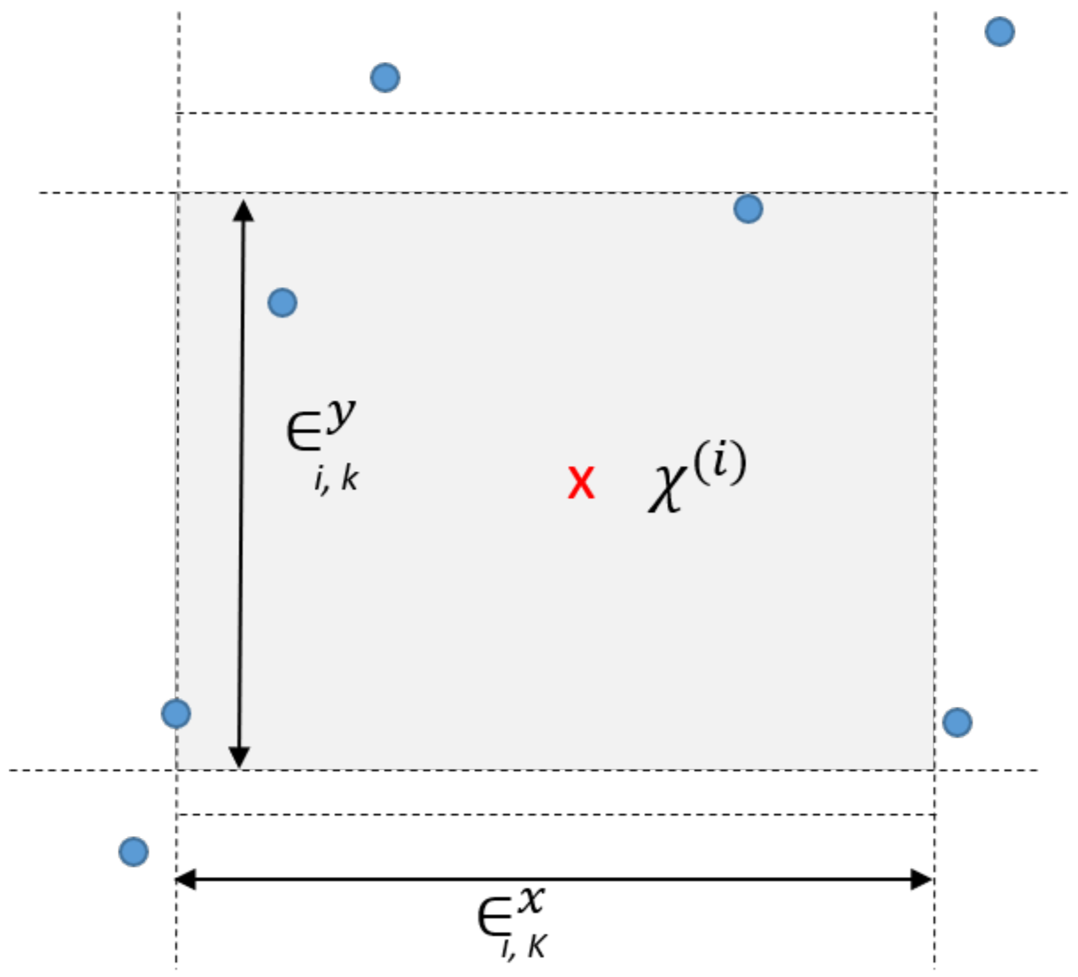
2.1. Transfer Entropy
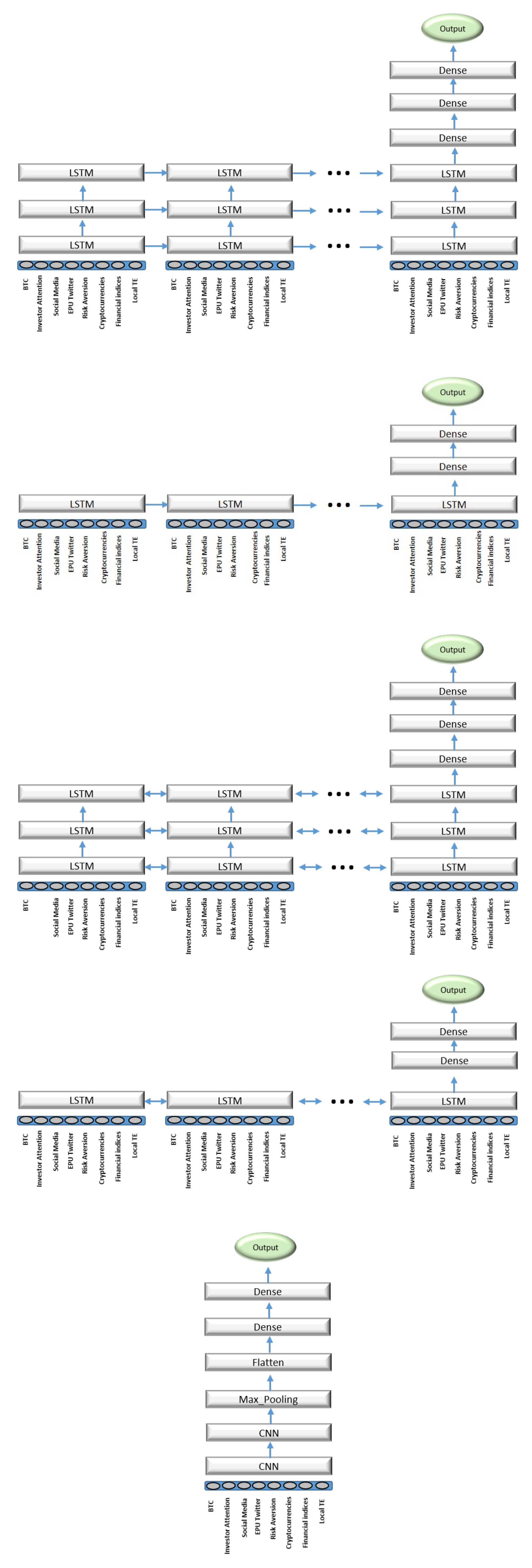
2.2. Deep Learning Models
2.3. Classification Metrics
- Accuracy =
- Sensitivity, recall or true positive rate (TPR)
- Specificity, selectivity or true negative rate (TNR)
- Precision or Positive Predictive Value (PPV)
- False Omission Rate (FOR)
- Balanced Accuracy (BA)
- F1 score .
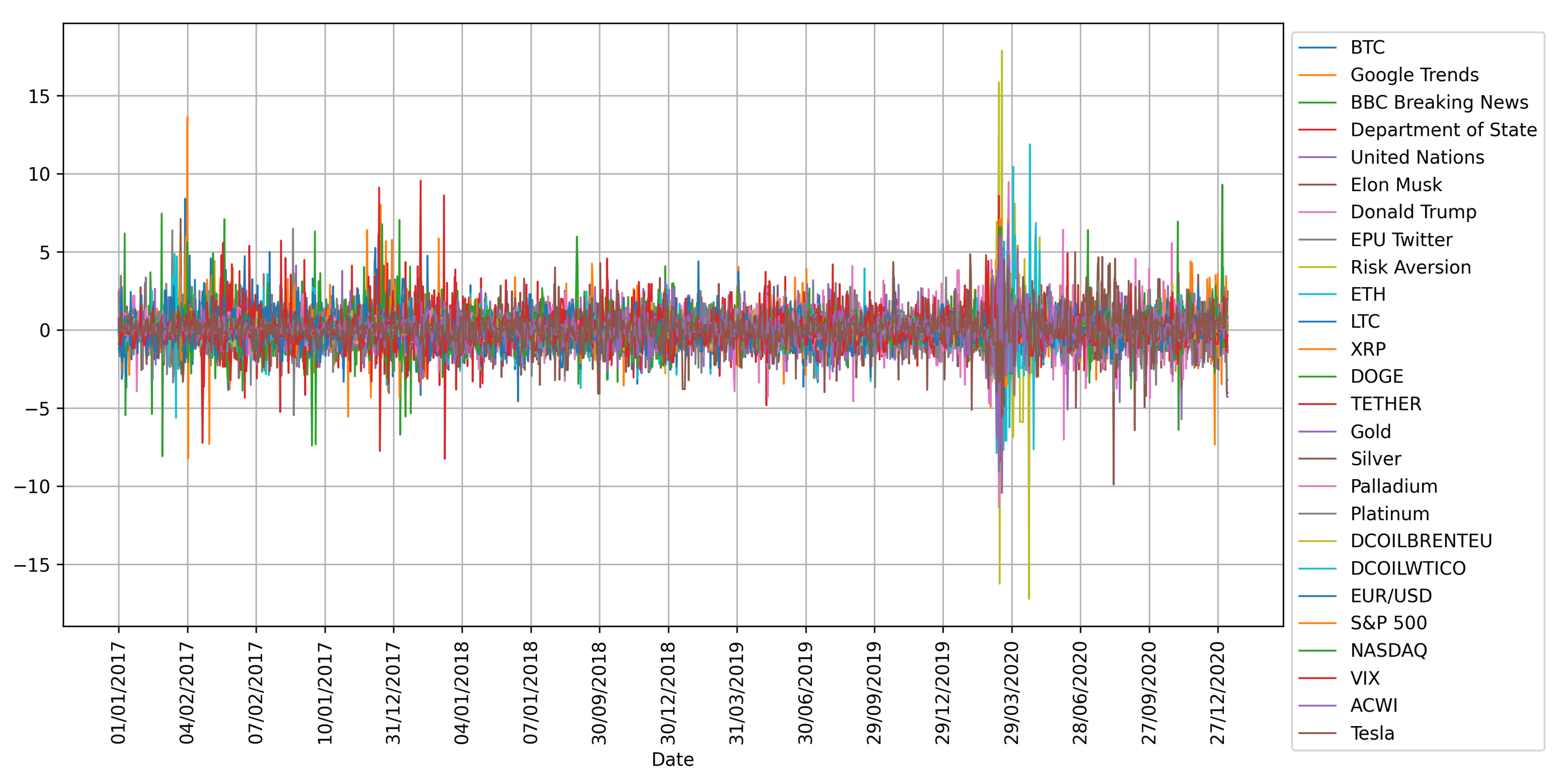
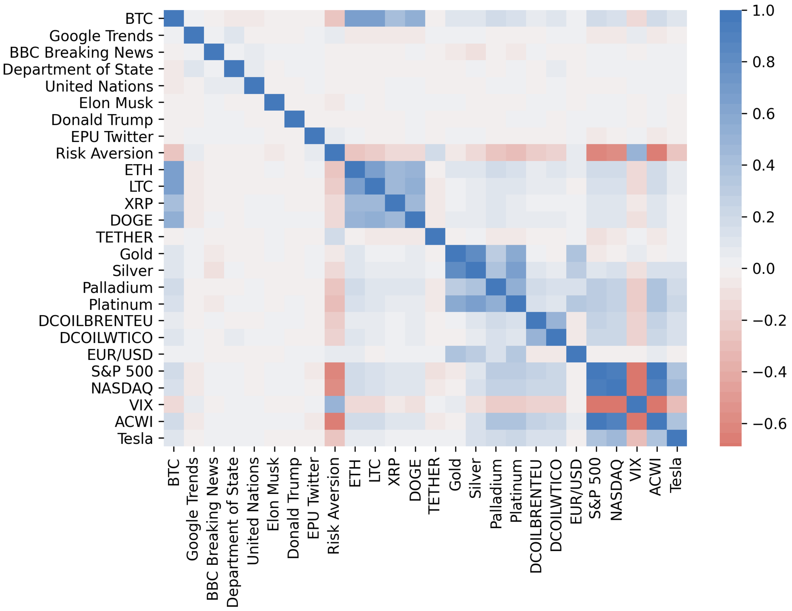
3. Data
4. Results
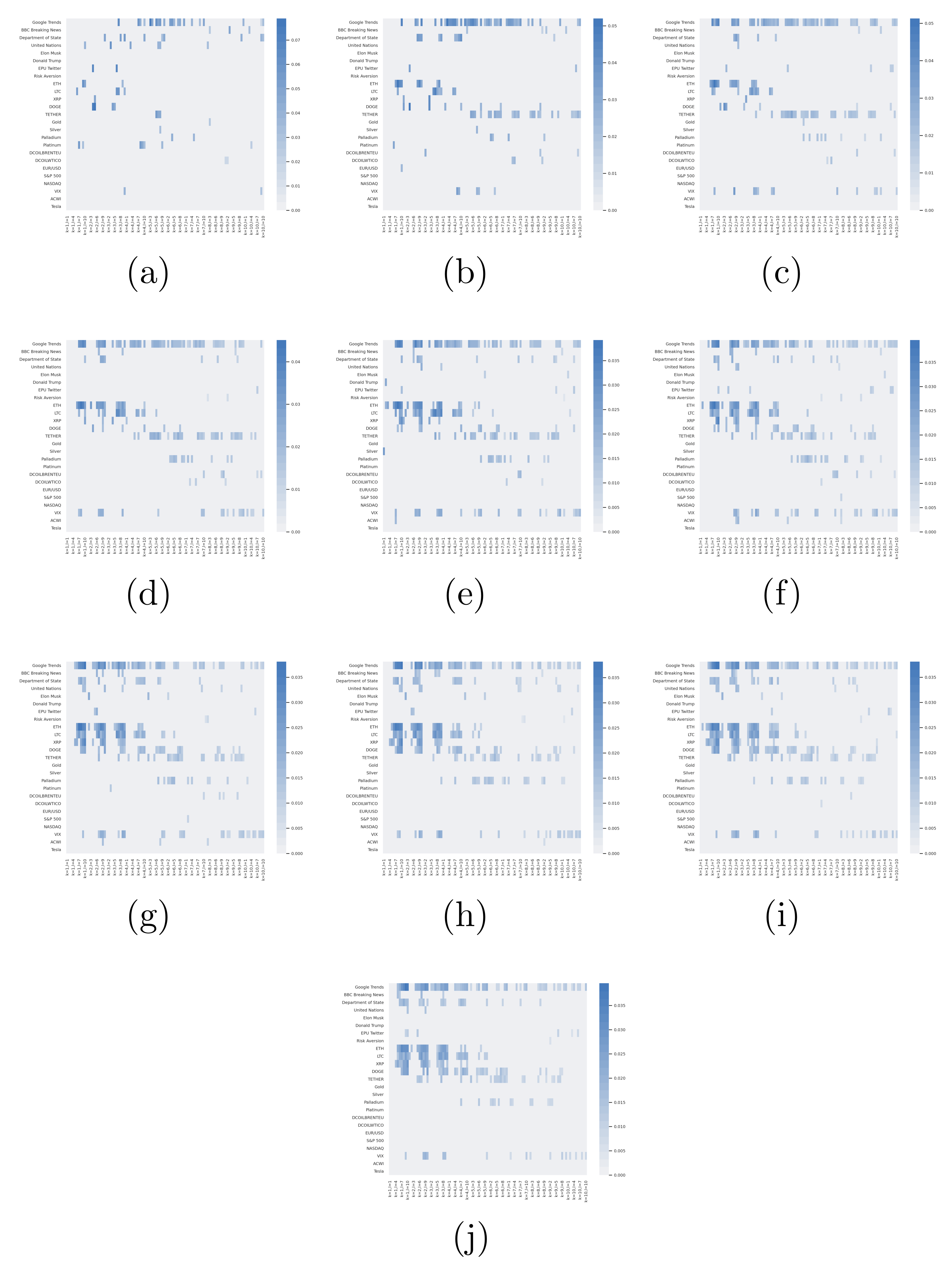
4.1. Variable Selection
4.2. Bitcoin’s Price Direction
5. Discussion
Supplementary Materials
Author Contributions
Funding
Institutional Review Board Statement
Informed Consent Statement
Data Availability Statement
Acknowledgments
Conflicts of Interest
References
- Wątorek, M.; Drożdż, S.; Kwapień, J.; Minati, L.; Oświęcimka, P.; Stanuszek, M. Multiscale characteristics of the emerging global cryptocurrency market. Phys. Rep. 2020, 901, 1–82. [Google Scholar] [CrossRef]
- Urquhart, A. What causes the attention of Bitcoin? Econ. Lett. 2018, 166, 40–44. [Google Scholar] [CrossRef] [Green Version]
- Shen, D.; Urquhart, A.; Wang, P. Does twitter predict Bitcoin? Econ. Lett. 2019, 174, 118–122. [Google Scholar] [CrossRef]
- Burggraf, T.; Huynh, T.L.D.; Rudolf, M.; Wang, M. Do FEARS drive Bitcoin? Rev. Behav. Financ. 2020, 13, 229–258. [Google Scholar] [CrossRef]
- Huynh, T.L.D. Does Bitcoin React to Trump’s Tweets? J. Behav. Exp. Financ. 2021, 31, 100546. [Google Scholar] [CrossRef]
- Corbet, S.; Larkin, C.; Lucey, B.M.; Meegan, A.; Yarovaya, L. The impact of macroeconomic news on Bitcoin returns. Eur. J. Financ. 2020, 26, 1396–1416. [Google Scholar] [CrossRef]
- Cavalli, S.; Amoretti, M. CNN-based multivariate data analysis for bitcoin trend prediction. Appl. Soft Comput. 2021, 101, 107065. [Google Scholar] [CrossRef]
- Gronwald, M. Is Bitcoin a Commodity? On price jumps, demand shocks, and certainty of supply. J. Int. Money Financ. 2019, 97, 86–92. [Google Scholar] [CrossRef]
- Baker, S.R.; Bloom, N.; Davis, S.J. Measuring economic policy uncertainty. Q. J. Econ. 2016, 131, 1593–1636. [Google Scholar] [CrossRef]
- Bekaert, G.; Engstrom, E.C.; Xu, N.R. The Time Variation in Risk Appetite and Uncertainty. Working Paper 25673, National Bureau of Economic Research, 2019. Available online: http://www.nber.org/papers/w25673 (accessed on 15 January 2021).
- Das, S.; Demirer, R.; Gupta, R.; Mangisa, S. The effect of global crises on stock market correlations: Evidence from scalar regressions via functional data analysis. Struct. Chang. Econ. Dyn. 2019, 50, 132–147. [Google Scholar] [CrossRef]
- Lahiani, A.; Jlassi, N.B.; Jeribi, A. Nonlinear tail dependence in cryptocurrency-stock market returns: The role of Bitcoin futures. Res. Int. Bus. Financ. 2021, 56, 101351. [Google Scholar] [CrossRef]
- Luu Duc Huynh, T. Spillover risks on cryptocurrency markets: A look from VAR-SVAR granger causality and student’st copulas. J. Risk Financ. Manag. 2019, 12, 52. [Google Scholar] [CrossRef] [Green Version]
- Huynh, T.L.D.; Nguyen, S.P.; Duong, D. Contagion risk measured by return among cryptocurrencies. In Proceedings of the International Econometric Conference of Vietnam, Ho Chi Minh, Vietnam, 15–16 January 2018; pp. 987–998. [Google Scholar]
- Huynh, T.L.D.; Nasir, M.A.; Vo, X.V.; Nguyen, T.T. “Small things matter most”: The spillover effects in the cryptocurrency market and gold as a silver bullet. N. Am. J. Econ. Financ. 2020, 54, 101277. [Google Scholar] [CrossRef]
- Thampanya, N.; Nasir, M.A.; Huynh, T.L.D. Asymmetric correlation and hedging effectiveness of gold & cryptocurrencies: From pre-industrial to the 4th industrial revolution. Technol. Forecast. Soc. Chang. 2020, 159, 120195. [Google Scholar]
- Huynh, T.L.D.; Burggraf, T.; Wang, M. Gold, platinum, and expected Bitcoin returns. J. Multinatl. Financ. Manag. 2020, 56, 100628. [Google Scholar] [CrossRef]
- Huynh, T.L.D.; Shahbaz, M.; Nasir, M.A.; Ullah, S. Financial modelling, risk management of energy instruments and the role of cryptocurrencies. Ann. Oper. Res. 2020, 1–29. [Google Scholar] [CrossRef]
- Huynh, T.L.D.; Ahmed, R.; Nasir, M.A.; Shahbaz, M.; Huynh, N.Q.A. The nexus between black and digital gold: Evidence from US markets. Ann. Oper. Res. 2021, 1–26. [Google Scholar] [CrossRef]
- Chu, J.; Nadarajah, S.; Chan, S. Statistical analysis of the exchange rate of bitcoin. PLoS ONE 2015, 10, e0133678. [Google Scholar]
- Lahmiri, S.; Bekiros, S.; Bezzina, F. Multi-fluctuation nonlinear patterns of European financial markets based on adaptive filtering with application to family business, green, Islamic, common stocks, and comparison with Bitcoin, NASDAQ, and VIX. Phys. A Stat. Mech. Its Appl. 2020, 538, 122858. [Google Scholar] [CrossRef]
- Ante, L. How Elon Musk’s Twitter Activity Moves Cryptocurrency Markets. 2021. SSRN 3778844. Available online: https://papers.ssrn.com/sol3/papers.cfm?abstract_id=3778844 (accessed on 15 June 2021).
- Schreiber, T. Measuring information transfer. Phys. Rev. Lett. 2000, 85, 461–464. [Google Scholar] [CrossRef] [PubMed] [Green Version]
- Philippas, D.; Rjiba, H.; Guesmi, K.; Goutte, S. Media attention and Bitcoin prices. Financ. Res. Lett. 2019, 30, 37–43. [Google Scholar] [CrossRef]
- Naeem, M.A.; Mbarki, I.; Suleman, M.T.; Vo, X.V.; Shahzad, S.J.H. Does Twitter Happiness Sentiment predict cryptocurrency? Int. Rev. Financ. 2020. [Google Scholar] [CrossRef]
- Kim, S.; Ku, S.; Chang, W.; Song, J.W. Predicting the Direction of US Stock Prices Using Effective Transfer Entropy and Machine Learning Techniques. IEEE Access 2020, 8, 111660–111682. [Google Scholar] [CrossRef]
- Gu, S.; Kelly, B.; Xiu, D. Empirical asset pricing via machine learning. Rev. Financ. Stud. 2020, 33, 2223–2273. [Google Scholar] [CrossRef] [Green Version]
- Kristoufek, L. What are the main drivers of the Bitcoin price? Evidence from wavelet coherence analysis. PLoS ONE 2015, 10, e0123923. [Google Scholar] [CrossRef] [PubMed]
- Giudici, P.; Polinesi, G. Crypto price discovery through correlation networks. Ann. Oper. Res. 2021, 299, 443–457. [Google Scholar] [CrossRef]
- Giudici, P.; Pagnottoni, P. Vector error correction models to measure connectedness of Bitcoin exchange markets. Appl. Stoch. Models Bus. Ind. 2020, 36, 95–109. [Google Scholar] [CrossRef] [Green Version]
- Ribeiro, M.T.; Singh, S.; Guestrin, C. “Why should i trust you? ” Explaining the predictions of any classifier. In Proceedings of the 22nd ACM SIGKDD International Conference on Knowledge Discovery and Data Mining, San Francisco, CA, USA, 13–17 August 2016; pp. 1135–1144. [Google Scholar]
- Lundberg, S.M.; Lee, S.I. A unified approach to interpreting model predictions. In Proceedings of the 31st International Conference on Neural Information Processing Systems, Long Beach, CA, USA, 4–9 December 2017; pp. 4768–4777. [Google Scholar]
- Schlegel, U.; Arnout, H.; El-Assady, M.; Oelke, D.; Keim, D.A. Towards a rigorous evaluation of xai methods on time series. In Proceedings of the 2019 IEEE/CVF International Conference on Computer Vision Workshop (ICCVW), Seoul, Korea, 27–28 October 2019; pp. 4197–4201. [Google Scholar]
- Bussmann, N.; Giudici, P.; Marinelli, D.; Papenbrock, J. Explainable AI in fintech risk management. Front. Artif. Intell. 2020, 3, 26. [Google Scholar] [CrossRef] [PubMed]
- Bussmann, N.; Giudici, P.; Marinelli, D.; Papenbrock, J. Explainable machine learning in credit risk management. Comput. Econ. 2021, 57, 203–216. [Google Scholar] [CrossRef]
- Bracke, P.; Datta, A.; Jung, C.; Sen, S. Machine Learning Explainability In Finance: An Application To Default Risk Analysis. 2019. Available online: https://www.bankofengland.co.uk/working-paper/2019/machine-learning-explainability-in-finance-an-application-to-default-risk-analysis (accessed on 15 November 2021).
- Ohana, J.J.; Ohana, S.; Benhamou, E.; Saltiel, D.; Guez, B. Explainable AI (XAI) models applied to the multi-agent environment of financial markets. In Proceedings of the International Workshop on Explainable, Transparent Autonomous Agents and Multi-Agent Systems, Virtual Event, 3–7 May 2021; Springer: Berlin/Heidelberg, Germany, 2021; pp. 189–207. [Google Scholar]
- Hailemariam, Y.; Yazdinejad, A.; Parizi, R.M.; Srivastava, G.; Dehghantanha, A. An Empirical Evaluation of AI Deep Explainable Tools. In Proceedings of the 2020 IEEE Globecom Workshops GC Wkshps, Madrid, Spain, 7–11 December 2020; pp. 1–6. [Google Scholar]
- Lizier, J.T.; Prokopenko, M.; Zomaya, A.Y. Local information transfer as a spatiotemporal filter for complex systems. Phys. Rev. E 2008, 77, 026110. [Google Scholar] [CrossRef] [Green Version]
- Bossomaier, T.; Barnett, L.; Harré, M.; Lizier, J.T. An introduction to Transfer Entropy; Springer: Berlin/Heidelberg, Germany, 2016; pp. 78–82. [Google Scholar]
- Kraskov, A.; Stögbauer, H.; Grassberger, P. Estimating mutual information. Phys. Rev. E 2004, 69, 066138. [Google Scholar] [CrossRef] [PubMed] [Green Version]
- Gao, S.; Ver Steeg, G.; Galstyan, A. Efficient estimation of mutual information for strongly dependent variables. arXiv 2015, arXiv:1411.2003. [Google Scholar]
- Hochreiter, S.; Schmidhuber, J. Long Short-Term Memory. Neural Comput. 1997, 9, 1735–1780. [Google Scholar] [CrossRef] [PubMed]
- Brownlee, J. Deep Learning for Time Series Forecasting: Predict the Future with MLPs, CNNs and LSTMs in Python; Machine Learning Mastery: 2018. Available online: https://machinelearningmastery.com/deep-learning-for-time-series-forecasting/ (accessed on 15 November 2021).
- Hutto, C.; Gilbert, E. Vader: A parsimonious rule-based model for sentiment analysis of social media text. Proc. Int. AAAI Conf. Web Soc. Media 2014, 8, 216–225. [Google Scholar]
- Reddi, S.J.; Kale, S.; Kumar, S. On the convergence of adam and beyond. arXiv 2018, arXiv:1904.09237. [Google Scholar]
- Grobys, K.; Sapkota, N. Cryptocurrencies and momentum. Econ. Lett. 2019, 180, 6–10. [Google Scholar] [CrossRef]
- Chaim, P.; Laurini, M.P. Is Bitcoin a bubble? Phys. A Stat. Mech. Its Appl. 2019, 517, 222–232. [Google Scholar] [CrossRef]
- Giudici, P.; Raffinetti, E. Shapley-Lorenz eXplainable artificial intelligence. Expert Syst. Appl. 2021, 167, 114104. [Google Scholar] [CrossRef]
- Giudici, P.; Raffinetti, E. Lorenz model selection. J. Classif. 2020, 37, 754–768. [Google Scholar] [CrossRef]


| Type | Variables |
|---|---|
| Investor attention | Google Trends |
| Social media | BBC Breaking News |
| Department of State | |
| United Nations | |
| Elon Musk | |
| Donald Trump | |
| Twitter-EPU | Twitter-based Uncertainty Index |
| Risk Aversion | Financial Proxy to Risk Aversion and Economic Uncertainty |
| Cryptocurrencies | ETH |
| LTC | |
| XRP | |
| DOGE | |
| TETHER | |
| Financial indices | Gold |
| Silver | |
| Palladium | |
| Platinum | |
| DCOILBRENTEU | |
| DCOILWTICO | |
| EUR/USD | |
| S&P 500 | |
| NASDAQ | |
| VIX | |
| ACWI | |
| Tesla |
| Variable | Mean | Std. Dev. | Skewness | Kurtosis | JB | p-Value |
|---|---|---|---|---|---|---|
| BTC | 0.0025 | 0.0424 | −0.8934 | 12.7470 | 10,073.5034 | *** |
| Google Trends | 0.0018 | 0.1915 | 0.2611 | 6.8510 | 2868.6001 | *** |
| BBC Breaking News | 0.0007 | 3.5295 | −0.1789 | 15.5376 | 14,686.4748 | *** |
| Department of State | −0.0013 | 4.0610 | 0.0941 | 8.4698 | 4362.1014 | *** |
| United Nations | 0.0007 | 3.2689 | 0.1748 | 0.2747 | 11.9228 | ** |
| Elon Musk | 0.0035 | 1.8877 | 0.0672 | 3.8630 | 906.9805 | *** |
| Donald Trump | 0.0001 | 4.8294 | 0.0461 | 5.2434 | 1670.4686 | *** |
| Twitter−EPU | 0.0009 | 0.3001 | 0.3049 | 3.6071 | 812.4777 | *** |
| Risk Aversion | 0.0001 | 0.0726 | 3.7594 | 165.2232 | 1,664,075.5884 | *** |
| ETH | 0.0034 | 0.0566 | −0.3991 | 9.7009 | 5759.1438 | *** |
| LTC | 0.0025 | 0.0606 | 0.6919 | 10.5404 | 6870.4947 | *** |
| XRP | 0.0027 | 0.0753 | 2.2903 | 36.2405 | 81,162.9262 | *** |
| DOGE | 0.0026 | 0.0669 | 1.2312 | 15.0342 | 14,113.2759 | *** |
| TETHER | 0.0000 | 0.0062 | 0.3255 | 20.0952 | 24,581.8501 | *** |
| Gold | 0.0006 | 0.0082 | −0.6595 | 5.5761 | 1995.0834 | *** |
| Silver | 0.0005 | 0.0164 | −1.1304 | 13.0841 | 10,720.4362 | *** |
| Palladium | 0.0015 | 0.0197 | −0.9198 | 20.5312 | 25,840.0775 | *** |
| Platinum | 0.0004 | 0.0145 | −0.9068 | 10.7274 | 7196.3125 | *** |
| DCOILBRENTEU | −0.0004 | 0.0374 | −3.1455 | 81.2272 | 403,755.7220 | *** |
| DCOILWTICO | 0.0006 | 0.0358 | 0.7362 | 38.4244 | 89,931.3161 | *** |
| EUR/USD | 0.0002 | 0.0042 | 0.0336 | 0.8999 | 49.0930 | *** |
| S&P 500 | 0.0006 | 0.0125 | −0.5714 | 20.5446 | 25,746.7436 | *** |
| NASDAQ | 0.0008 | 0.0145 | −0.3601 | 11.7771 | 8463.6169 | *** |
| VIX | −0.0061 | 0.0810 | 1.4165 | 8.4537 | 4833.8826 | *** |
| ACWI | 0.0006 | 0.0115 | −1.1415 | 20.4837 | 25,833.5682 | *** |
| Tesla | 0.0017 | 0.0371 | −0.3730 | 5.5089 | 1877.5034 | *** |
| Design | Case | Dropout | LR | Batch | Acc | AUC | TPR | TNR | PPV | FOR | BA | F1 | # |
|---|---|---|---|---|---|---|---|---|---|---|---|---|---|
| D1 | S1 | 0.3 | 0.001 | 32 | 57.11 | 0.5388 | 84.75 | 25.28 | 56.63 | 40.97 | 55.02 | 67.89 | |
| S2 | 0.3 | 0.001 | 128 | 57.28 | 0.5391 | 80.33 | 30.75 | 57.18 | 42.40 | 55.54 | 66.80 | ||
| S3 | 0.7 | 0.001 | 128 | 58.07 | 0.5379 | 74.43 | 39.25 | 58.51 | 42.86 | 56.84 | 65.51 | ||
| S4 | 0.3 | 0.001 | 256 | 57.98 | 0.5304 | 75.41 | 37.92 | 58.30 | 42.74 | 56.67 | 65.76 | ||
| S5 | 0.3 | 0.001 | 256 | 57.19 | 0.5100 | 87.54 | 22.26 | 56.45 | 39.18 | 54.90 | 68.64 | ||
| D2 | S1 | 0.3 | 0.001 | 64 | 59.82 | 0.5444 | 81.97 | 34.34 | 58.96 | 37.67 | 58.15 | 68.59 | |
| S2 | 0.3 | 0.001 | 32 | 61.14 | 0.5909 | 65.57 | 56.04 | 63.19 | 41.42 | 60.81 | 64.36 | ||
| S3 | 0.3 | 0.001 | 128 | 62.28 | 0.6062 | 62.95 | 61.51 | 65.31 | 40.94 | 62.23 | 64.11 | 5 | |
| S4 | 0.5 | 0.0001 | 32 | 55.44 | 0.4964 | 75.08 | 32.83 | 56.27 | 46.63 | 53.96 | 64.33 | ||
| S5 | 0.7 | 0.001 | 32 | 58.07 | 0.5706 | 63.77 | 51.51 | 60.22 | 44.74 | 57.64 | 61.94 | ||
| D3 | S1 | 0.3 | 0.001 | 128 | 56.23 | 0.4865 | 88.52 | 19.06 | 55.73 | 40.94 | 53.79 | 68.40 | |
| S2 | 0.3 | 0.001 | 64 | 59.65 | 0.5816 | 68.69 | 49.25 | 60.90 | 42.26 | 58.97 | 64.56 | ||
| S3 | 0.3 | 0.001 | 128 | 60.09 | 0.5619 | 76.72 | 40.94 | 59.92 | 39.55 | 58.83 | 67.29 | ||
| S4 | 0.3 | 0.001 | 32 | 58.16 | 0.5350 | 79.18 | 33.96 | 57.98 | 41.37 | 56.57 | 66.94 | ||
| S5 | 0.3 | 0.001 | 256 | 59.47 | 0.5702 | 68.69 | 48.87 | 60.72 | 42.44 | 58.78 | 64.46 | ||
| D4 | S1 | 0.5 | 0.001 | 32 | 57.28 | 0.5276 | 80.16 | 30.94 | 57.19 | 42.46 | 55.55 | 66.76 | |
| S2 | 0.7 | 0.001 | 128 | 58.68 | 0.5447 | 66.23 | 50.00 | 60.39 | 43.74 | 58.11 | 63.17 | ||
| S3 | 0.7 | 0.001 | 64 | 58.25 | 0.5468 | 64.26 | 51.32 | 60.31 | 44.49 | 57.79 | 62.22 | ||
| S4 | 0.5 | 0.001 | 256 | 57.11 | 0.5092 | 78.36 | 32.64 | 57.25 | 43.28 | 55.50 | 66.16 | ||
| S5 | 0.7 | 0.0001 | 32 | 57.11 | 0.5328 | 70.33 | 41.89 | 58.21 | 44.91 | 56.11 | 63.70 | ||
| D5 | S1 | 0.7 | 0.001 | 128 | 60.09 | 0.5834 | 72.13 | 46.23 | 60.69 | 40.96 | 59.18 | 65.92 | |
| S2 | 0.3 | 0.001 | 64 | 60.00 | 0.5683 | 67.70 | 51.13 | 61.46 | 42.09 | 59.42 | 64.43 | ||
| S3 | 0.5 | 0.001 | 32 | 59.39 | 0.5648 | 68.03 | 49.43 | 60.76 | 42.67 | 58.73 | 64.19 | ||
| S4 | 0.5 | 0.001 | 32 | 59.12 | 0.5572 | 75.57 | 40.19 | 59.25 | 41.16 | 57.88 | 66.43 | ||
| S5 | 0.3 | 0.001 | 128 | 60.79 | 0.5825 | 70.33 | 49.81 | 61.73 | 40.67 | 60.07 | 65.75 |
| Design | Case | Acc | AUC | TPR | TNR | PPV | FOR | BA | F1 | # |
|---|---|---|---|---|---|---|---|---|---|---|
| D1 | S1 | 64.30 | 0.4981 | 90.99 | 11.67 | 67.01 | 60.38 | 51.33 | 77.18 | |
| S2 | 56.82 | 0.4946 | 74.08 | 22.78 | 65.42 | 69.17 | 48.43 | 69.48 | ||
| S3 | 61.78 | 0.5188 | 79.58 | 26.67 | 68.15 | 60.17 | 53.12 | 73.42 | 2 | |
| S4 | 51.96 | 0.4898 | 60.70 | 34.72 | 64.71 | 69.06 | 47.71 | 62.65 | ||
| S5 | 60.47 | 0.4842 | 83.66 | 14.72 | 65.93 | 68.64 | 49.19 | 73.74 | ||
| D2 | S1 | 60.75 | 0.4786 | 85.92 | 11.11 | 65.59 | 71.43 | 48.51 | 74.39 | |
| S2 | 52.06 | 0.4870 | 56.48 | 43.33 | 66.28 | 66.45 | 49.91 | 60.99 | ||
| S3 | 53.46 | 0.4997 | 56.76 | 46.94 | 67.85 | 64.50 | 51.85 | 61.81 | ||
| S4 | 55.70 | 0.4794 | 70.56 | 26.39 | 65.40 | 68.75 | 48.48 | 67.89 | ||
| S5 | 50.93 | 0.4806 | 55.49 | 41.94 | 65.34 | 67.67 | 48.72 | 60.02 | ||
| D3 | S1 | 65.05 | 0.5072 | 95.21 | 5.56 | 66.54 | 62.96 | 50.38 | 78.33 | 3 |
| S2 | 55.70 | 0.5248 | 63.38 | 40.56 | 67.77 | 64.04 | 51.97 | 65.50 | ||
| S3 | 57.38 | 0.5176 | 67.32 | 37.78 | 68.09 | 63.04 | 52.55 | 67.71 | ||
| S4 | 51.40 | 0.5051 | 52.96 | 48.33 | 66.90 | 65.75 | 50.65 | 59.12 | ||
| S5 | 54.21 | 0.5094 | 60.56 | 41.67 | 67.19 | 65.12 | 51.12 | 63.70 | ||
| D4 | S1 | 61.21 | 0.4831 | 86.48 | 11.39 | 65.81 | 70.07 | 48.93 | 74.74 | |
| S2 | 48.13 | 0.4718 | 48.17 | 48.06 | 64.65 | 68.02 | 48.11 | 55.21 | ||
| S3 | 47.20 | 0.4771 | 43.24 | 55.00 | 65.46 | 67.05 | 49.12 | 52.08 | ||
| S4 | 45.98 | 0.4359 | 50.99 | 36.11 | 61.15 | 72.80 | 43.55 | 55.61 | ||
| S5 | 51.96 | 0.4743 | 55.49 | 45.00 | 66.55 | 66.11 | 50.25 | 60.52 | ||
| D5 | S1 | 58.04 | 0.5017 | 78.59 | 17.50 | 65.26 | 70.70 | 48.05 | 71.31 | |
| S2 | 55.23 | 0.4942 | 62.39 | 41.11 | 67.63 | 64.34 | 51.75 | 64.91 | ||
| S3 | 54.21 | 0.4994 | 63.10 | 36.67 | 66.27 | 66.50 | 49.88 | 64.65 | ||
| S4 | 54.49 | 0.5269 | 62.39 | 38.89 | 66.82 | 65.60 | 50.64 | 64.53 | ||
| S5 | 55.79 | 0.5316 | 61.83 | 43.89 | 68.49 | 63.17 | 52.86 | 64.99 | 2 |
Publisher’s Note: MDPI stays neutral with regard to jurisdictional claims in published maps and institutional affiliations. |
© 2021 by the authors. Licensee MDPI, Basel, Switzerland. This article is an open access article distributed under the terms and conditions of the Creative Commons Attribution (CC BY) license (https://creativecommons.org/licenses/by/4.0/).
Share and Cite
García-Medina, A.; Luu Duc Huynh, T. What Drives Bitcoin? An Approach from Continuous Local Transfer Entropy and Deep Learning Classification Models. Entropy 2021, 23, 1582. https://doi.org/10.3390/e23121582
García-Medina A, Luu Duc Huynh T. What Drives Bitcoin? An Approach from Continuous Local Transfer Entropy and Deep Learning Classification Models. Entropy. 2021; 23(12):1582. https://doi.org/10.3390/e23121582
Chicago/Turabian StyleGarcía-Medina, Andrés, and Toan Luu Duc Huynh. 2021. "What Drives Bitcoin? An Approach from Continuous Local Transfer Entropy and Deep Learning Classification Models" Entropy 23, no. 12: 1582. https://doi.org/10.3390/e23121582
APA StyleGarcía-Medina, A., & Luu Duc Huynh, T. (2021). What Drives Bitcoin? An Approach from Continuous Local Transfer Entropy and Deep Learning Classification Models. Entropy, 23(12), 1582. https://doi.org/10.3390/e23121582