1. Introduction
Stochastic gradient (
sg) methods have been extensively studied as a means for
mcmc-based Bayesian posterior sampling algorithms to scale to large data regimes. Variants of
sg-mcmc algorithms have been studied through the lens of first [
1,
2,
3] or second-order [
4,
5] Langevin Dynamics, which are mathematically convenient continuous-time processes that correspond to discrete-time gradient methods with and without momentum, respectively. The common traits underlying many methods from the literature can be summarized as follows: they address large data requirements using
sg and mini-batching, they inject Gaussian noise throughout the algorithm execution, and they avoid the expensive Metropolis-Hasting accept/reject tests that use the whole data [
1,
2,
4].
Despite mathematical elegance and some promising results restricted to simple models, current approaches fall short in dealing with the complexity of the loss landscape typical of popular modern machine learning models, e.g., neural networks [
6,
7], for which stochastic optimization poses some serious challenges [
8,
9].
In general,
sg-mcmc algorithms inject random noise to
sg descent algorithms: the covariance of such noise and the learning rate, or step-size in the stochastic differential equation simulation community, are tightly related to the assumptions on the loss landscape, which together with the
sg noise, determine the sampling properties of these methods [
5]. However, current
sg-mcmc algorithms applied to popular complex models such as Deep Nets, cannot simultaneously satisfy the assumptions on posterior distribution geometry and on the behavior of the covariance of the
sg noise, while operating with the practical requirement of non-vanishing learning rates. In this paper, in accordance with most of the Neural Network related literature, we refer to the posterior distribution geometry as loss landscape. Some recent work [
10], instead, argue for fixed step sizes, but settle for variational approximations of quadratic losses. Although we are not the first to highlight these issues, including the lack of a unified notation [
5], we believe that studying the role of noise in
sg-mcmc algorithms has not received enough attention, and a deeper understanding is truly desirable, as it can clarify how various methods compare. Most importantly, this endeavor can suggest novel and more practical algorithms relying on fewer parameters and less restrictive assumptions.
In this work we chose a mathematical notation that emphasizes the role of noise covariances and learning rate on the behavior of
sg-mcmc algorithms (
Section 2). As a result, the equivalence between learning rate annealing and extremely large injected noise covariance becomes apparent, and this allows us to propose a novel practical
sg-mcmc algorithm (
Section 3). We derive our proposal, by first analyzing the case where we inject the smallest complementary noise such that its combined effects with the
sg noise result in an isotropic noise. Thanks to this isotropic property of the noise, it is possible to deal with intricate loss surfaces typical of deep models, and produce samples from the true posterior without learning rate annealing. This, however, comes at the expense of cubic complexity matrix operations. We address such issues through a practical variant of our scheme, which employs well-known approximations to the
sg noise covariance (see, e.g., [
11]). The result is an algorithm that produces approximate posterior samples with a fixed, theoretically derived, learning rate. Please note that in generic Bayesian deep learning setting, none of the existing implementations of
sg-mcmc methods converge to the true posterior without learning rate annealing. In contrast, our method automatically determines an appropriate learning rate through a simple estimation procedure. Furthermore, our approach can be readily applied to pre-trained models: after a “warmup” phase to compute
sg noise estimates, it can efficiently perform Bayesian posterior sampling.
We evaluate
sg-mcmc algorithms (
Section 4) through an extensive experimental campaign, where we compare our approach to several alternatives, including Monte Carlo Dropout (
mcd) [
12] and Stochastic Weighted Averaging Gaussians (
swag, [
9]), which have been successfully applied to the Bayesian deep learning setting. Our results indicate that our approach offers performance that are competitive to the state of the art, according to metrics that aim at assessing the predictive accuracy and uncertainty.
2. Preliminaries and Related Work
Consider a dataset of
m—dimensional observations
. Given prior
for a
d-dimensional set of parameters, and a likelihood model
, the posterior is obtained by means of Bayes theorem as follows:
where
is also known as the model evidence, defined as the integral
. Except when the prior and the likelihood function are conjugate, Equation (
1) is analytically intractable [
13]. However, the joint likelihood term in the numerator is typically not hard to compute; this is a key element of many
mcmc algorithms, since the normalization constant
does not affect the shape of the distribution in any way other than scaling. The posterior distribution is necessary to obtain predictive distributions for new test observations
, as:
We focus in particular on Monte Carlo methods to obtain an estimate of this predictive distribution, by averaging over
samples obtained from the posterior over
, i.e.,
We develop our work by working with an unnormalized version of the logarithm of the posterior density, by expressing the negative logarithm of the joint distribution of the dataset
and parameters
as:
For computational efficiency, we use a minibatch stochastic gradient
, which guarantees that the estimated gradient is an unbiased estimate of the true gradient
, and we assume that the randomness due to the minibatch introduces a Gaussian noise:
where the matrix
denotes the
sg noise covariance, which depends on the parametric model, the data distribution and the minibatch size.
A survey of algorithms to sample from the posterior using
sg methods can be found in Ma et al. [
5]. In
Appendix A we report some well-known facts which are relevant for the derivations in our paper. As shown in the literature [
10,
14], there are structural similarities between
sg-mcmc algorithms and stochastic optimization methods, and both can be used to draw samples from posterior distributions. Notice that the original goal of stochastic optimization is to find the minimum of a given cost function, and the stochasticity is introduced by sub-sampling the dataset to scale.
sg-mcmc methods instead aim at sampling from a given distribution, i.e., collecting multiple values, and the stochasticity is necessary explore the whole landscape. In what follows, we use a unified notation to compare many existing algorithms in light of the role played by their noise components.
It is well-known [
15,
16,
17] that stochastic gradient descent (
sgd), with and without momentum, can be studied through the following stochastic differential equation (
sde), when the learning rate
is small enough (In this work we do not consider discretization errors. The reader can refer to classical
sde texts such as [
18] to investigate the topic in greater depth.):
where
is usually referred to as driving force and
as diffusion matrix We use a generic form of the
sde, with variable
instead of
, which accommodates
sgd variants, with and without momentum. By doing this, we will be able to easily cast the expression for the two cases in what follows (The operator
applied to matrix
produces a row vector whose elements are the divergences of the
columns. Our notation is aligned with Chen et al. [
4]).
Definition 1. A distribution is said to be astationarydistribution for thesdeof the form (6), if and only if it satisfies the following Fokker-Planck equation (fpe): Please note that in general, the stationary distribution does not converge to the desired posterior distribution, i.e.,
, as shown by Chaudhari and Soatto [
8]. Additionally, given an initial condition for
, its distribution is going to converge to
only for
. In practice, we observe the
sde dynamics for a finite amount of time: then, we declare that the process is approximately in the stationary regime once the potential has reached low and stable values.
Next, we briefly overview known approaches to Bayesian posterior sampling, and interpret them as variants of an sgd process, using the fpe formalism.
2.1. Gradient Methods without Momentum
The generalized updated rule of
sgd, described as a discrete-time stochastic process, writes as:
where
is a user-defined preconditioning matrix, and
is a noise term, distributed as
, with a user-defined covariance matrix
. Then, the corresponding continuous-time
sde is [
15]:
In this paper we use the symbol
n to indicate discrete time, while
t for continuous time. We denote by
the covariance of the
injected noise and
the
composite noise covariance. Please note that
combines the
sg and the injected noise. Notice that our choice of notation is different from the standard one, in which the starting discrete-time process is in the form
. By directly grouping the injected noise with the stochastic gradient we can better appreciate the relationship between annealing the learning rate and extremely large injected noise. Moreover, as will be explained in
Section 3, this allows derivation of a new sampling algorithm.
We define the stationary distribution of the
sde in Equation (
9) as
. Please note that when
, the potential
differs from the desired posterior
[
8]. The following theorem, which is an adaptation of known results in light of our formalism, states the conditions for which the
noisy sgd converges to the true posterior distribution (proof in
Appendix A).
Theorem 1. Consider dynamics of the form (9) and define the stationary distribution . Ifthen . Stochastic Gradient Langevin Dynamics (
sgld) [
1] is a simple approach to satisfy Equation (
10); it uses no preconditioning,
, and sets the injected noise covariance to
. In the limit for
, it holds that
. Then,
, and
. Although
sgld succeeds in (asymptotically) generating samples from the true posterior, its mixing rate is unnecessarily slow, due to the extremely small learning rate [
2].
An extension to
sgld is Stochastic Gradient Fisher Scoring (
sgfs) [
2], which can be tuned to switch between sampling from an approximate posterior, using a non-vanishing learning rate, and the true posterior, by annealing the learning rate to zero.
sgfs uses preconditioning,
. In practice, however,
is ill conditioned for complex models such as deep neural networks. Then, many of its eigenvalues are almost zero [
8], and computing
is problematic. An in-depth analysis of
sgfs reveals that conditions (
10) would be met with a non-vanishing learning rate only if, at convergence,
, which would be trivially true if
was constant. However, recent work [
6,
7] suggest that this condition is difficult to justify for deep neural networks.
The Stochastic Gradient Riemannian Langevin Dynamics (
sgrld) algorithm [
3] extends
sgfs to the setting in which
. The process dynamic is adjusted by adding the term
. However, the term
has not a clear estimation procedure, restricting
sgrld to cases where it can be computed analytically.
The work by [
10] investigates constant-rate
sgd (with no injected noise), and determines analytically the learning rate and preconditioning that minimize the Kullback–Leibler (
kl) divergence between an approximation and the true posterior. Moreover, it shows that the preconditioning used in
sgfs is optimal, in the sense that it converges to the true posterior, when
is constant and the true posterior has a quadratic form.
In summary, to claim convergence to the true posterior distribution, existing approaches require either vanishing learning rates or assumptions on the sg noise covariance that are difficult to verify in practice, especially when considering deep models. We instead propose a novel practical method that induces isotropic sg noise and thus satisfies Theorem 1. We determine analytically a fixed learning rate, and we require weaker assumptions on the loss shape.
2.2. Gradient Methods with Momentum
Momentum-corrected methods emerge as a natural extension to
sgd approaches. The general set of update equations for (discrete-time) momentum-based algorithms is:
where
is a preconditioning matrix,
M is the mass matrix and
is the friction matrix, as shown by [
4,
19]. As with the first order counterpart, the noise term is distributed as
. Then, the
sde to describe continuous-time system dynamics is:
where
and we assume
to be symmetric. The theorem hereafter describes the conditions for which noisy
sgd with momentum converges to the true posterior distribution (
Appendix A).
Theorem 2. Consider dynamics of the form (11) and define the stationary distribution for as . Ifthen . In the naive case, where
, Equation (
12) are not satisfied and the stationary distribution does not correspond to the true posterior [
4]. To generate samples from the true posterior it is sufficient to set
(as in Equation (
9) in [
4]).
Stochastic Gradient Hamiltonian Monte Carlo (
sghmc) [
4] suggests that estimating
can be costly. Hence, the injected noise
is chosen such that
, where
is user-defined. When
, the following approximation holds:
. It is then trivial to check that conditions (
12) hold without the need for explicitly estimating
. A further practical reason to avoid setting
is that the computational cost for the operation
has
complexity, whereas if
is diagonal, this is reduced to
. This, however, severely slows down the sampling process.
Stochastic Gradient Riemannian Hamiltonian Monte Carlo (
sgrhmc) is an extension to
sghmc [
5]), which considers a generic, space-varying preconditioning matrix
derived from information geometric arguments [
20].
sgrhmc suggests setting
, where
is the Fisher Information matrix. To meet the requirement
, it includes a correction term,
. The injected noise is set to
, consequently
, and the friction matrix is set to
. With all these choices, Theorem 2 is satisfied. Although appealing, the main drawbacks of this method are the need for an analytical expression of
, and the assumption for
to be known.
From a practical standpoint, momentum-based methods suffer from the requirement to tune many hyperparameters, including the learning rate, and the parameters that govern the simulation of a second-order Langevin dynamics.
The method we propose in this work can be applied to momentum-based algorithms; in this case, it could be viewed as an extension of the work in [
11], albeit addressing the complex loss landscapes typical of deep neural networks. However, we leave this avenue of research for future work.
3. Sampling by Layer-Wise Isotropization
We present a simple and practical approach to inject noise to SGD iterates to perform Bayesian posterior sampling. Our goal is to sample from the true posterior distribution (or approximations thereof) using a
constant learning rate, and to rely on more lenient assumptions about the shape of the loss landscape that characterize deep models, compared to previous works. In general, in modern machine learning applications, we deal with multi-layer neural networks [
21]. We exploit the natural subdivision of the parameters of these architecture into different layers to propose a practical sampling scheme
Careful inspection of Theorem 1 reveals that the matrices
are instrumental in determining the convergence properties of
sg methods to the true posterior. Therefore, we consider the constructive approach of
designing to obtain a sampling scheme that meets our goals; we set
to be a constant, diagonal matrix which we constrain to be layer-wise uniform:
By properly selecting the set of parameters we can achieve the simultaneous result of non-vanishing learning rate and well-conditioned preconditioning matrix. This implies a layer-wise learning rate for the p-th layer, without further preconditioning.
We can now prove (see
Appendix B), as a corollary to Theorem 1, that our design choices can guarantee convergence to the true posterior distribution.
Corollary 1. (Theorem 1) Consider dynamics of the form (9) and define the stationary distribution . If as in (13), and , then . If aforementioned conditions are satisfied, it is in fact simple to show that the relevant matrices satisfy the conditions in Equation (
10). The covariance matrix of the composite noise is said to be
isotropic within the layers of (deep) models. In fact,
. From a practical point of view, we choose
to be, among all valid matrices satisfying
, the smallest (the one with the smallest
’s). Indeed, larger
induce a smaller learning rate, thus unnecessarily reducing sampling speed.
Now, let us consider an ideal case, in which we assume the
sg noise covariance
and
to be known in advance. The procedure described in Algorithm 1 illustrates a naive
sg method that uses the
injected noise covariance
to sample from the true posterior.
| Algorithm 1 Idealized posterior sampling |
| {Initialization: } |
|
|
| loop |
| |
| |
| |
| |
| |
| end loop |
This deceivingly simple procedure generate samples from the true posterior, with a non-vanishing learning rate, as shown earlier. However, it cannot be used in practice as and are unknown. Furthermore, the algorithm requires computationally expensive operations, i.e., to compute , which requires operations, and , which costs multiplications.
Next, we describe a practical variant of our approach, where we use approximations at the expense of generating samples from the true posterior distribution. We note that [
10] suggest exploring a related preconditioning, but do not develop this path in their work. Moreover, the proposed method shares similarities with a scheme proposed in [
22] although the analysis we perform here is different.
3.1. A Practical Method: Isotropic SGD
To render the idealized sampling method practical, it is necessary to consider some additional assumptions. As we explain at the end of this section, the assumptions that follow are less strict than other approaches in the literature.
Assumption 1. Thesgnoise covariance can be approximated with a diagonal matrix, i.e., .
Assumption 2. The signal-to-noise ratio (SNR) of a gradient is small enough such that in the stationary regime, the second-order moment of the gradient is a good estimate of the true variance. Hence, combining with Assumption 1, , where ⊙ indicates the elementwise product.
Assumption 3. The sum of the variances of noise components, layer by layer, can be assumed to constant in the stationary regime. Then, , where is the set of indices of parameters belonging to layer.
The diagonal covariance assumption (i.e., Assumption 1) is common in other works, such as [
2,
11]. The small signal-to-noise ratio as stated in Assumption 2 is in line with recent studies, such as [
11,
23]. Assumption 3 is similar to those appeared in earlier work, such as [
24]. Please note that Assumptions 2 and 3 must hold in the stationary regime when the process reaches the bottom valley of the loss landscape. The matrix
has been associated in the literature with the
empirical Fisher information matrix [
2,
25]. As we do not consider this matrix for preconditioning purposes, we do not further investigate this connection.
Given our assumptions, and our design choices, it is then possible to show (see
Appendix B) that the optimal (i.e., the smallest possible)
satisfying Corollary 1 can be obtained as
. Please note that we do not assume
to be known, but use a simple procedure to estimate its components by computing:
where
is the portion of stochastic gradient corresponding to the
p-th layer. Then, the composite noise matrix
is a layer-wise isotropic covariance matrix, which inspires the name of our proposed method as
Isotropic SGD (
i-sgd).
The practical implementation of
i-sgd is shown in Algorithm 2. The advantage of
i-sgd is that it can either be used to obtain posterior samples starting from a pre-trained model, or do so by training a model from scratch. In either case, the estimates of
are used to compute
, as discussed above. An important consideration is that once all
have been estimated, the learning rate, layer by layer, is determined
automatically. In fact, for the
p-th layer, the learning rate is:
. A simpler approach is to use a unique learning rate for all layers, where the equivalent
is the sum of all
.
| Algorithm 2i-sgd: practical posterior sampling |
|
|
| loop |
| |
| for to Nl do |
| |
| |
| |
| end for |
| |
| end loop |
3.2. Computational Cost
The computational cost of
i-sgd is as follows. As with [
4], we define the cost of computing a gradient minibatch as
. Thanks to Assumptions 1 and 2, the computational cost for estimating the noise covariance scales as
multiplications. The computational cost of generating random samples with the desired covariance scales as
square roots and
multiplications (without considering the cost of generating random numbers). The overall cost of our method is the sum of the above terms. Notice that the cost of estimating the noise covariance does not depend on the minibatch size
. We would like to stress that in many modern models, the real computational bottleneck is the backward propagation for the computation of the gradients. As all the
sg-mcmc methods considered in this work require one gradient evaluation per step, the different methods have in practice the same complexity.
The space complexity of i-sgd is the same as sghmc,sgfs and variants: it scales as , where is the number of posterior samples.
4. Experiments
The empirical analysis of our method, and its comparison to alternative approaches from the literature, is organized as follows. First, we proceed with a validation of
i-sgd using the standard
uci datasets [
26] and a shallow neural network. Then we move to the case of deeper models: we begin with a simple CNN used on the
mnist [
27] dataset, then move to the standard
ResNet-18 [
28] deep network using the
Cifar-10 [
29] dataset.
We compare
i-sgd to other Bayesian sampling methods such as
sghmc [
4],
sgld [
2], and to alternative approaches to approximate Bayesian inference, including
mcd [
12],
swag [
9] and
vsgd [
10]. In general, our result indicates that: (1)
i-sgd achieves similar or superior performance regarding competitors, when measuring uncertainty quantification, even with simple datasets and models; (2)
i-sgd is simple to tune, when compared to alternatives; (3)
i-sgd is competitive when used for deep Bayesian modeling, even when compared to standard methods used in the literature. In particular, the proposed method shares some of the strengths of
vsgd, such as learning rates determined automatically and the simplicity of
sgld.
Appendix B includes additional implementation details on
i-sgd.
Appendix C presents detailed configurations of all methods we compare, and additional experimental results.
4.1. A Disclaimer on Performance Characterization
It is important to stress a detail on the analysis of the experimental campaign. The discussion is usually focused on the goodness of the various methods for representing the true posterior distribution. Different methods can or cannot claim convergence to the true posterior according to certain assumptions and the nature of the hyperparameters. In the experimental validation of the results, however, we do not have access to the form of the true posterior as it is exactly the problem we are trying to solve. The practical solution adopted is to compare the different methods in terms of proxy metrics evaluated on the test sets, such as the accuracy and uncertainty metrics. Being better in terms of these performance metrics does not imply that the sampling method is better at approximating the posterior distribution, and outperforming competitors in terms of these metric do not provide sufficient information about the intrinsic quality of the sampling scheme.
4.2. Regression Tasks, with Simple Models
We consider several regression tasks defined on the
uci datasets. We use a simple neural network configuration with two fully connected layers and a
re
lu activation function; the hidden layer includes 50 units. In this set of experiments, we use the following metrics: the root mean square error (
rmse) to judge the model predictive performance and the mean negative log-likelihood (
mnll) as a proxy for uncertainty quantification. We note that the task of tuning our competitors was far from trivial. We used our own version of
sghmc, based on [
11], to ensure a proper understanding of the implementation internals, and we proceeded with a tuning process to find appropriate values for the numerous hyperparameters. In this set of experiments, we omit results for
swag, which we keep for more involved scenarios.
Table 1 and
Table 2 report a complete overview of our results, for a selection of
uci datasets. For each method and each dataset, we also included how many out of the 10 splits considered failed to converge, indicated as
. As explained in
Appendix C we implemented a temperature scaled version of
vsgd. A clear picture emerges from this first set of experiments: while for the
rmse the performance is similar for different methods, for the
mnll averaging over multiple samples clearly improves the uncertainty quantification capabilities.
sghmc is in many cases better than alternatives, considering however the standard deviation of the results it is difficult to claim clear superiority of one method over the others.
4.3. Classification Tasks, with Deeper Models
Next, we compare
i-sgd against competitors on image classification tasks. First, we use the
mnist dataset, and a simple
LeNet-5 CNN [
30]. All methods are compared based on the test accuracy
acc,
mnll and the expected calibration error (
ece,
31]). Additionally, at test time, we carry out predictions on both
mnist and
not-mnist; the latter is a dataset equivalent to
mnist, but it represents letters rather than numbers. (
http://yaroslavvb.blogspot.com/2011/09/notmnist-dataset.html, accessed on 24 October 2021) This experimental setup is often used to check whether the entropy of the predictions on
not-mnist is higher than the entropy of the predictions on
mnist (the entropy of the output of an
classes classifier, represented by the vector
, is defined as
).
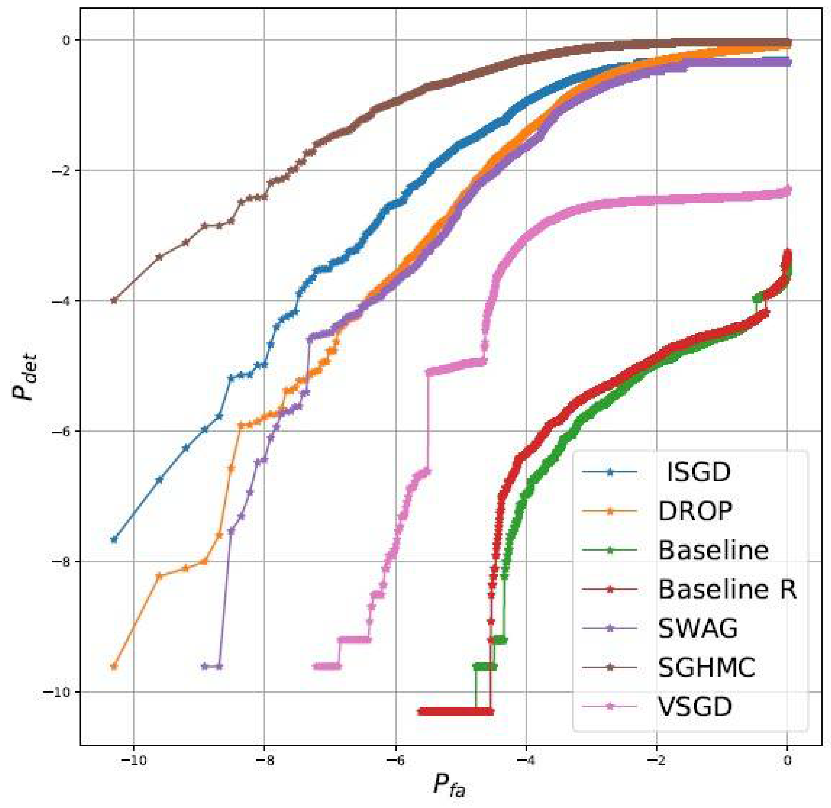
Table 3 indicates that all methods are essentially equivalent in terms of accuracy and
mnll. We consider, together with the classical in and out of distribution entropies the regions of convergence (
rocs) diagrams comparing detection of out of distribution samples and false alarms when using as test statistic the entropy. Results, reported in
Figure 1, clearly shows that: (1) collecting multiple samples improve the uncertainty quantification capabilities (2)
i-sgd is competitive (but not the best scheme) and importantly outperform the closest approach to ours, i.e.,
vsgd. The experimental results show that
i-sgd improves the quality of the
baseline model with respect to all metrics. To test whether the improvements are due just to “
additional training” or are intrinsically due to the Bayesian averaging properties, we do consider alternative deterministic baselines (details in
Appendix C). For this set of experiments the best performing is
baseline R. As can be appreciated by comparing
Table 3 and
Figure 1, while it is possible to increase the classical metrics,
i-sgd (and other methods) still outperform by a large margin the baselines in terms of detection of out of distribution samples.
We now move on to a classical image classification problem with deep convolutional networks, whereby we use the
cifar10 dataset, and the
ResNet-18 network architecture. For this set of experiments, we compare
i-sgd,
sghmc,
swag, and
vsgd using again test accuracy and
mnll, which we report in
Table 4. As usual, we compare the results against the baseline of the individual network resulting from the pre-training phase. Results are obtained averaging over three independent seeds. Notice, as expanded in
Appendix C that for
swag we do consider two variants: the Bayesian correct one (
swag) and a second variant that has better performance (
swag wd). We stress again, as highlighted in
Section 4.1 that not always goodness of approximation of the posterior and performance correlate positively. Additionally in this case, we found
i-sgd to be competitive with other methods and superior to the baseline. Among the competitors, we found
i-sgd to the easiest to tune, given the feature of a fixed learning rate informed by theoretical considerations; we believe that this is an important aspect to consider for a wide adoption of our proposal by practitioners.
5. Conclusions
sg methods allowed Bayesian posterior sampling algorithms, such as mcmc, to regain relevance in an age when datasets have reached extremely large sizes. However, despite mathematical elegance and promising results, current approaches from the literature are restricted to simple models. Indeed, the sampling properties of these algorithms are determined by simplifying assumptions on the loss landscape, which do not hold for the kind of complex models which are popular these days, such as deep models. Meanwhile, sg-mcmc algorithms require vanishing learning rates, which force practitioners to develop creative annealing schedules that are often model specific and difficult to justify.
We have attempted to target these weaknesses by suggesting a simpler algorithm that relies on fewer parameters and less strict assumptions compared to the literature on sg-mcmc. We used a unified mathematical notation to deepen our understanding of the role of the covariance of the noise of stochastic gradients and learning rate on the behavior of sg-mcmc algorithms. We then presented a practical variant of the sgd algorithm, which uses a constant learning rate, and an additional noise to perform Bayesian posterior sampling. Our proposal is derived from the ideal method, in which it is guaranteed that samples are generated from the true posterior. When the learning rate and noise terms are empirically estimated, with no user intervention, our method offers a very good approximation to the posterior, as demonstrated by the extensive experimental campaign.
We verified empirically the quality of our approach, and compared its performance to state-of-the-art sg-mcmc and alternative methods. Results, which span a variety of settings, indicated that our method is competitive to the alternatives from the state-of-the-art, while being much simpler to use.


