Option Portfolio Selection with Generalized Entropic Portfolio Optimization


Abstract
1. Introduction
1.1. Literature Review
2. Maximum Exponential Growth Rate
2.1. The Kelly Criterion for Multiple Wagers
2.2. Extension of the Kelly Criterion to Option Strategies
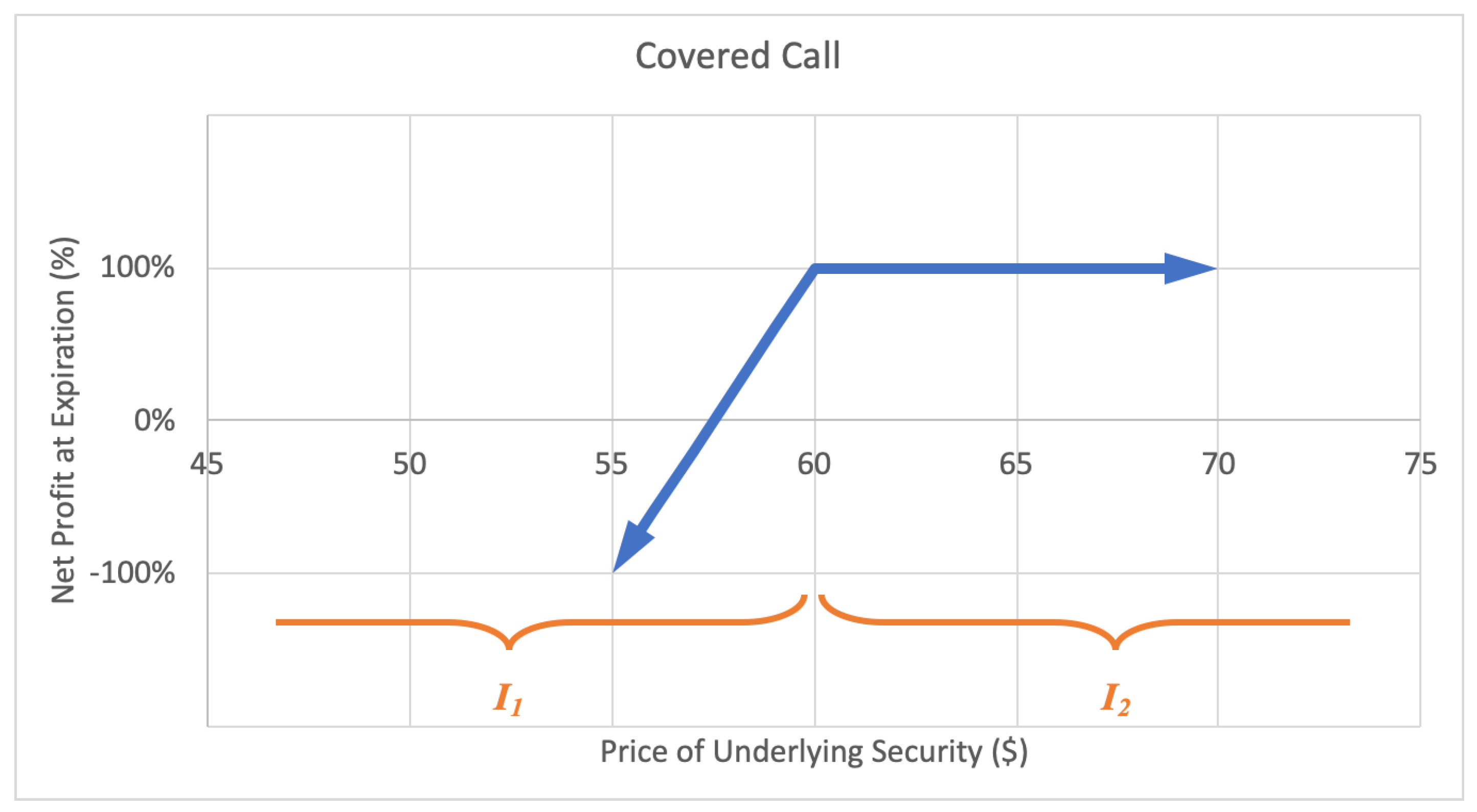
2.2.1. Covered Call
2.2.2. Married Put
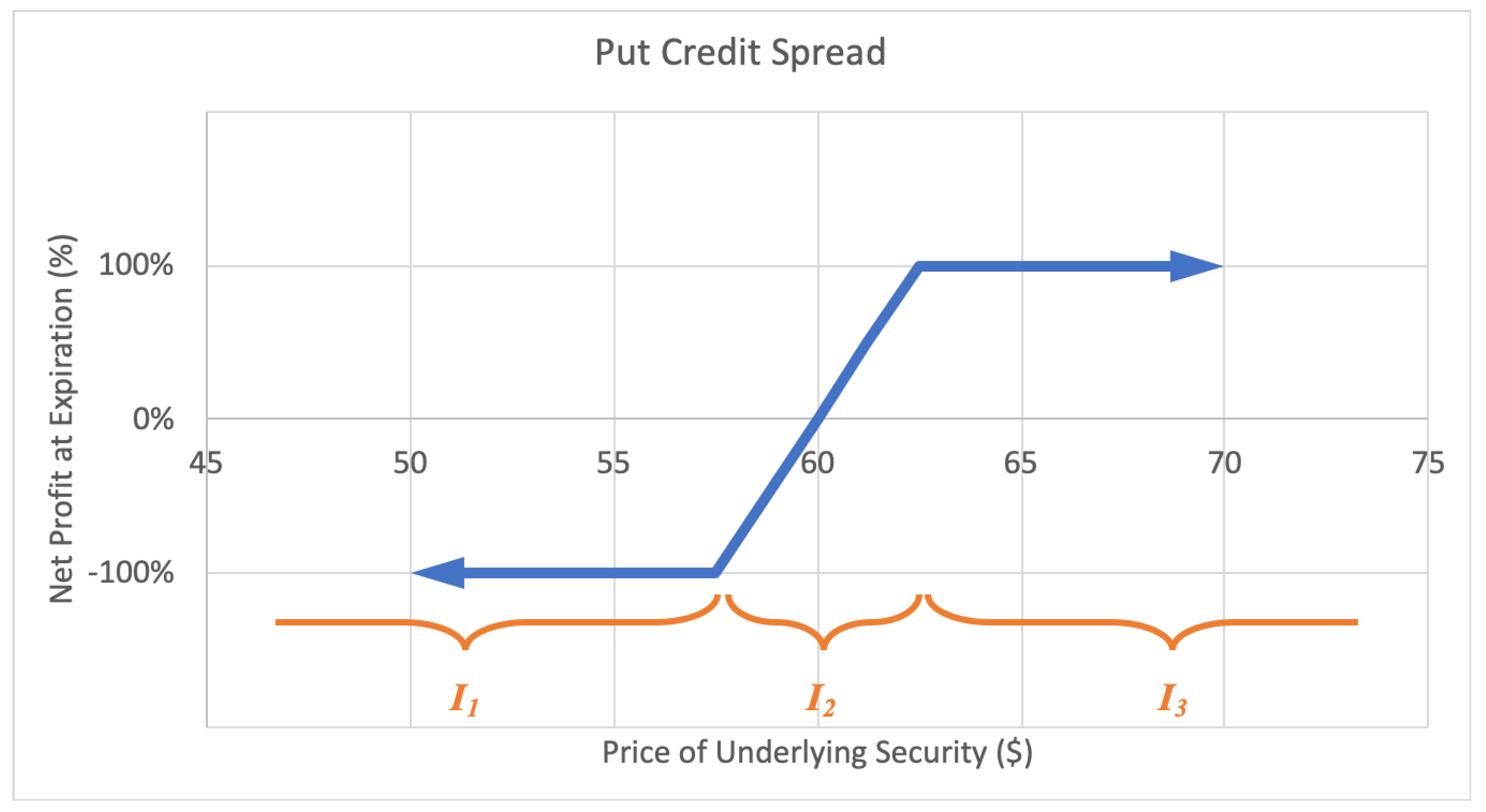
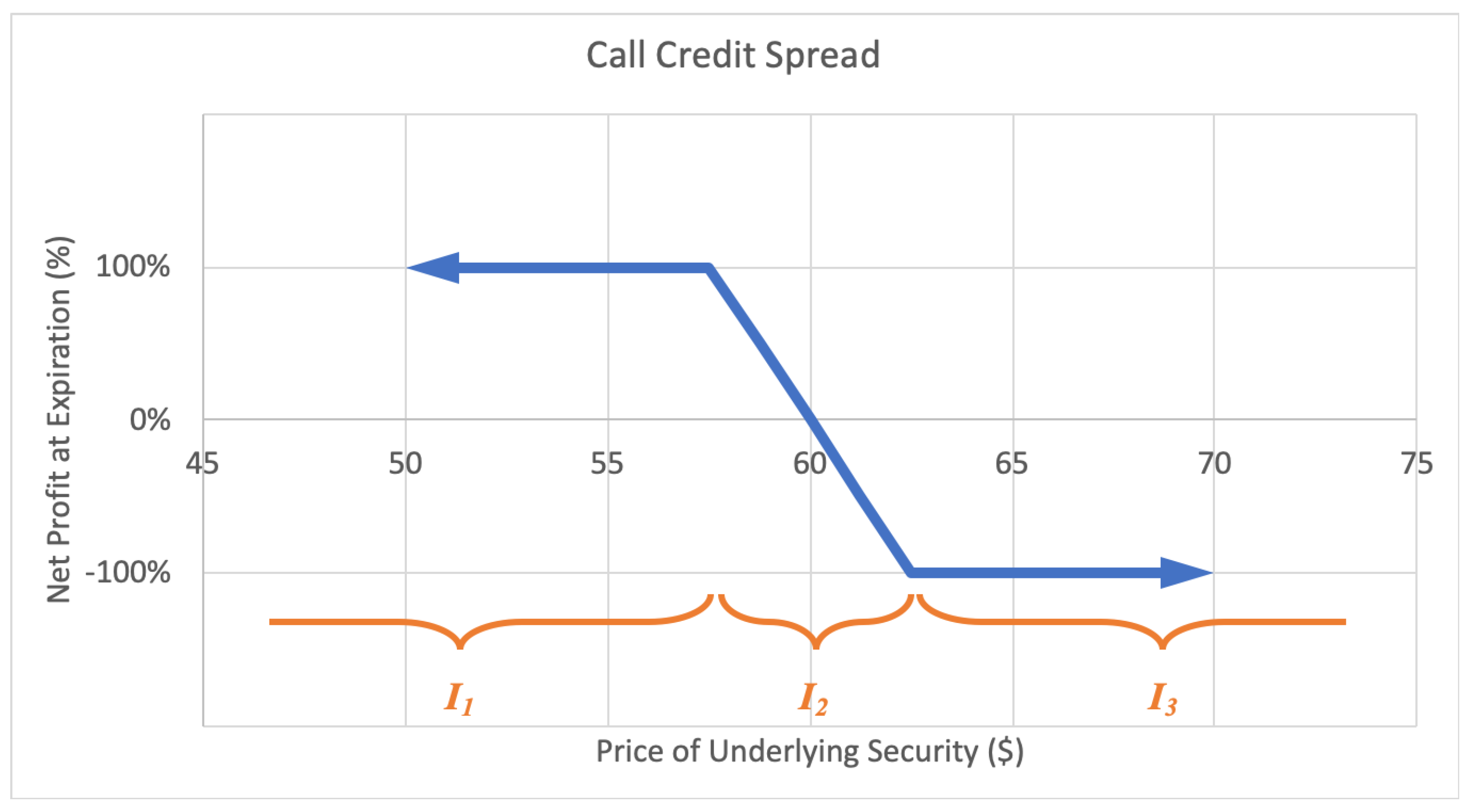
2.2.3. Credit Spread
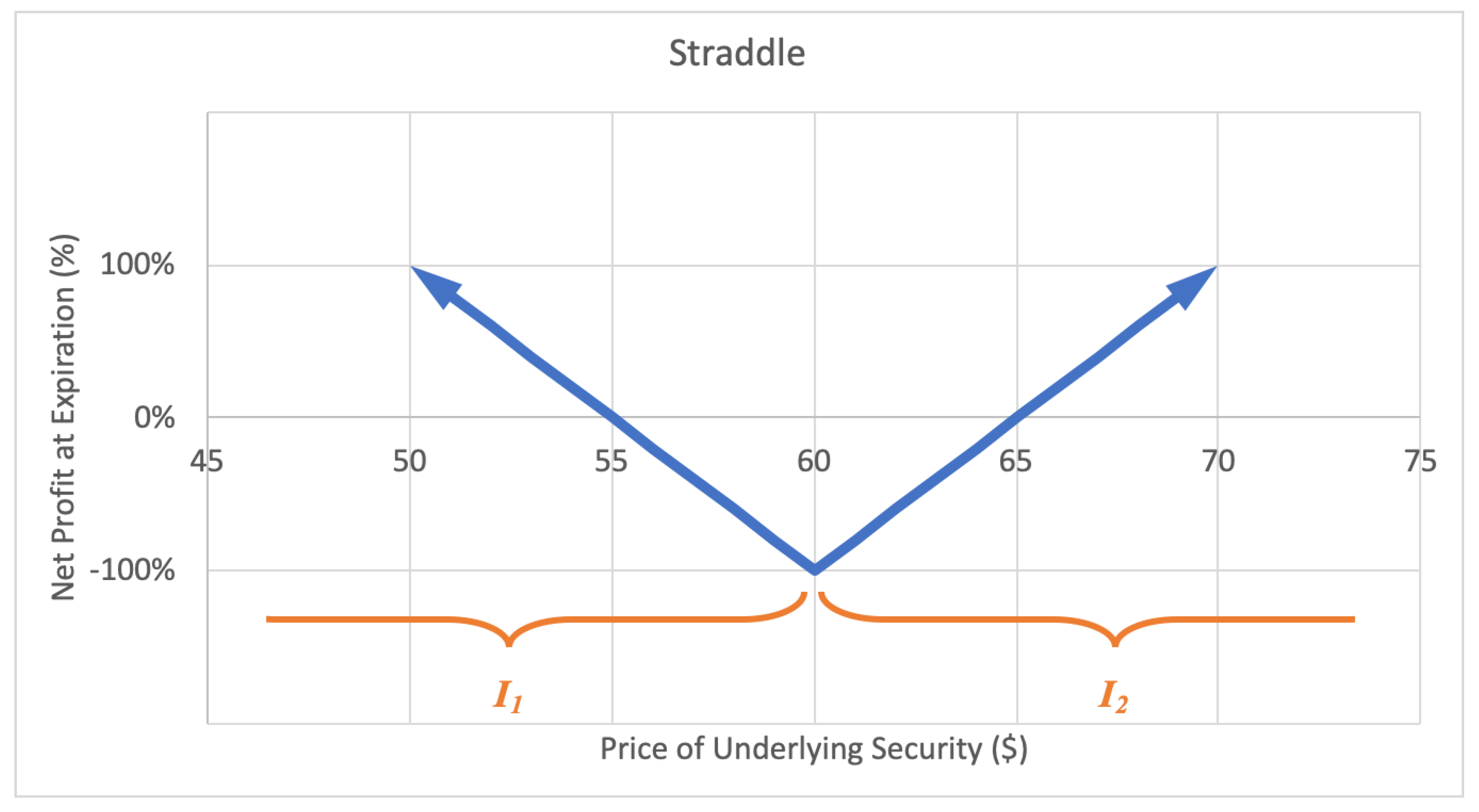
2.2.4. Straddle
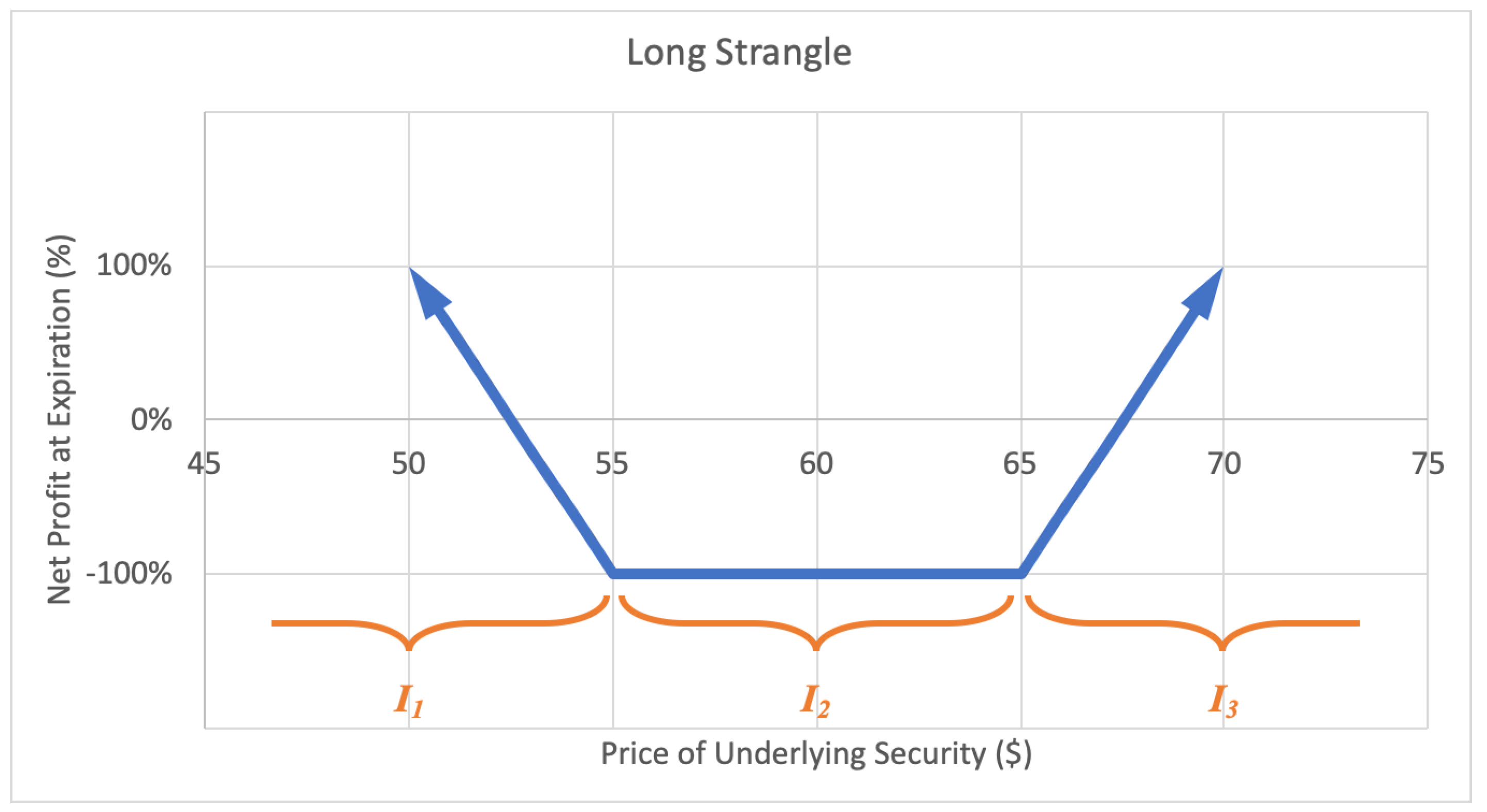
2.2.5. Long Strangle
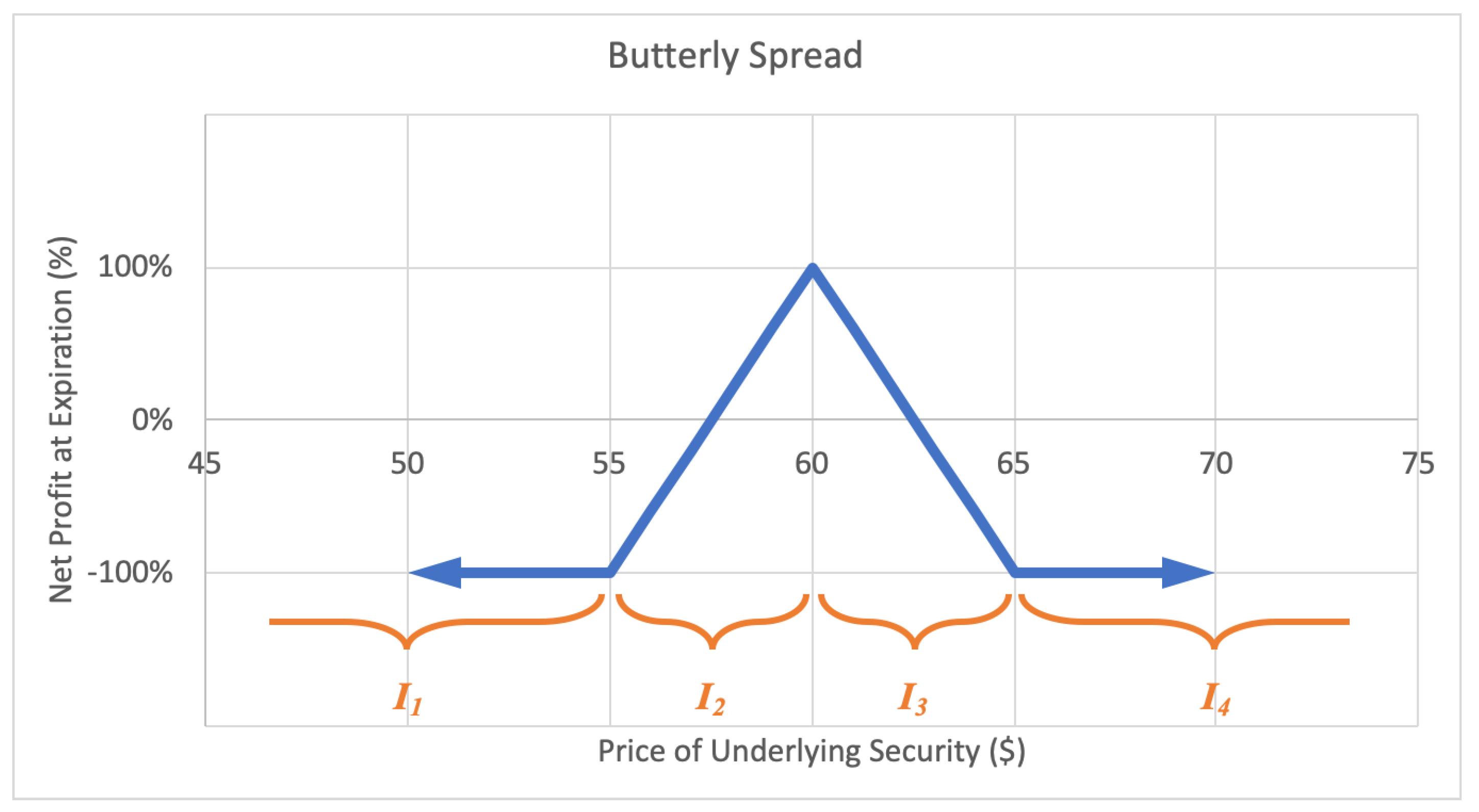
2.2.6. Butterfly Spread
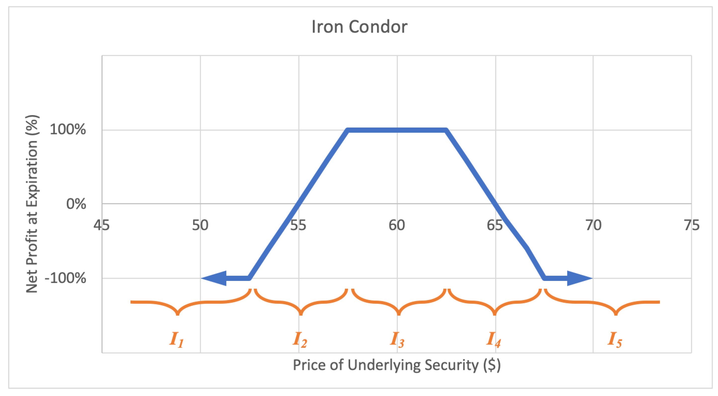
2.2.7. Iron Condor
3. Minimum Relative Entropy
3.1. Shannon Entropy
3.2. Kullback–Leibler Divergence
4. Option Portfolio Selection Based on Growth Rate and Relative Entropy
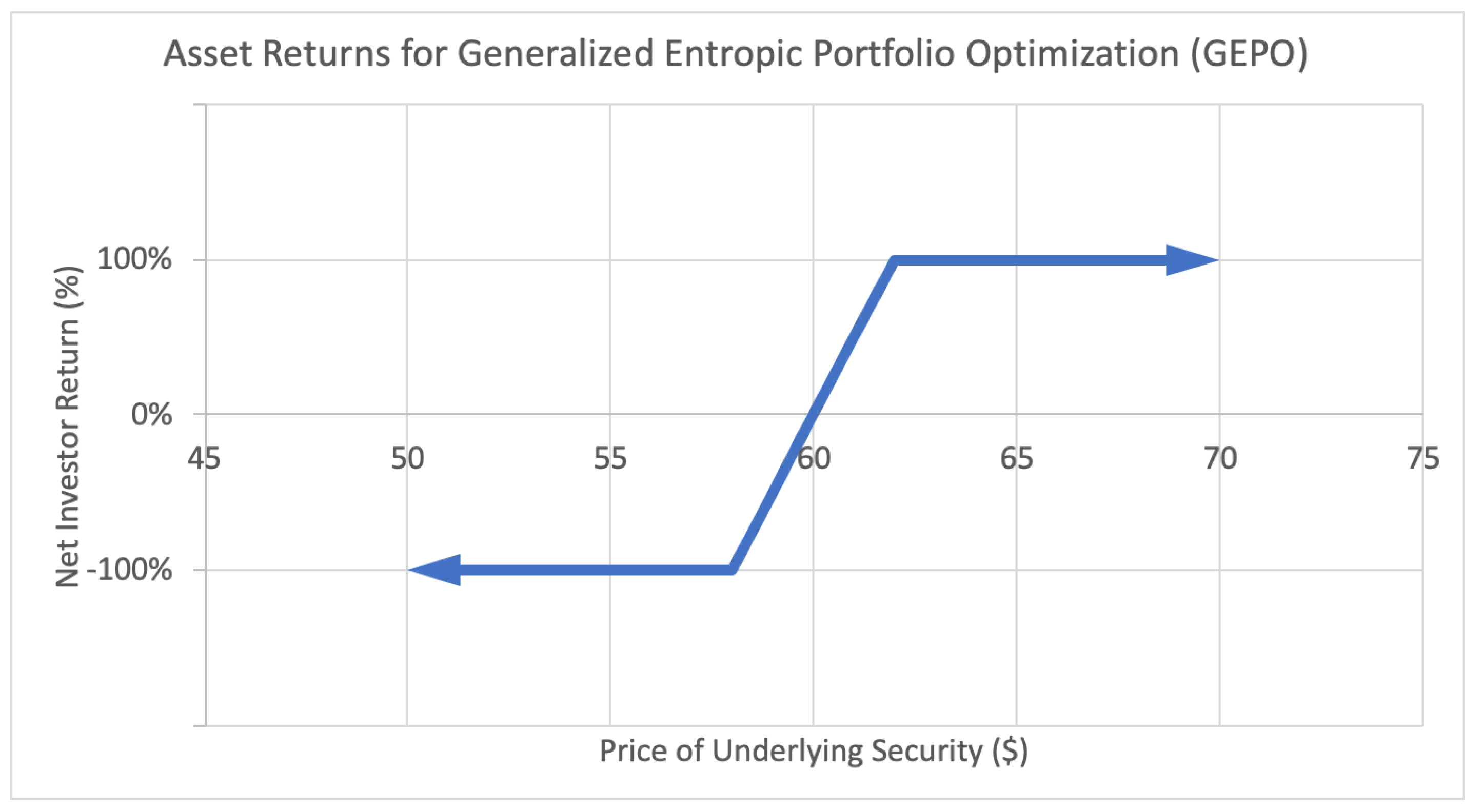
4.1. Generalized Entropic Portfolio Optimization (GEPO)
4.2. Risk-Adjusted Performance
5. An Option Portfolio Selection Example with GEPO
5.1. Data
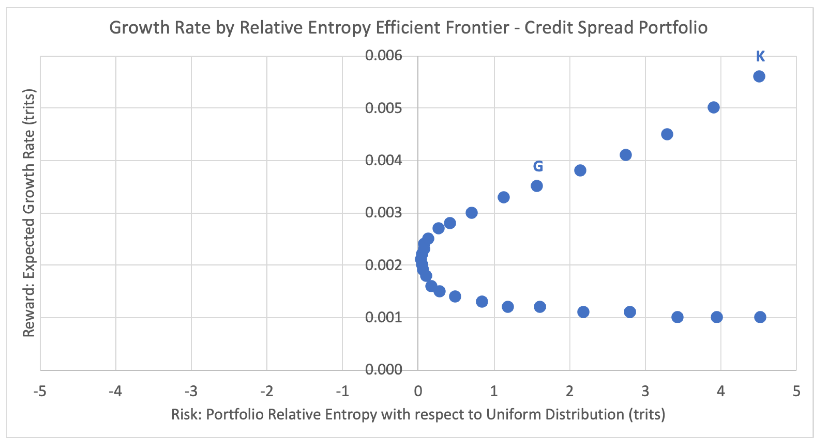
5.2. Efficient Frontier and Portfolio Selection
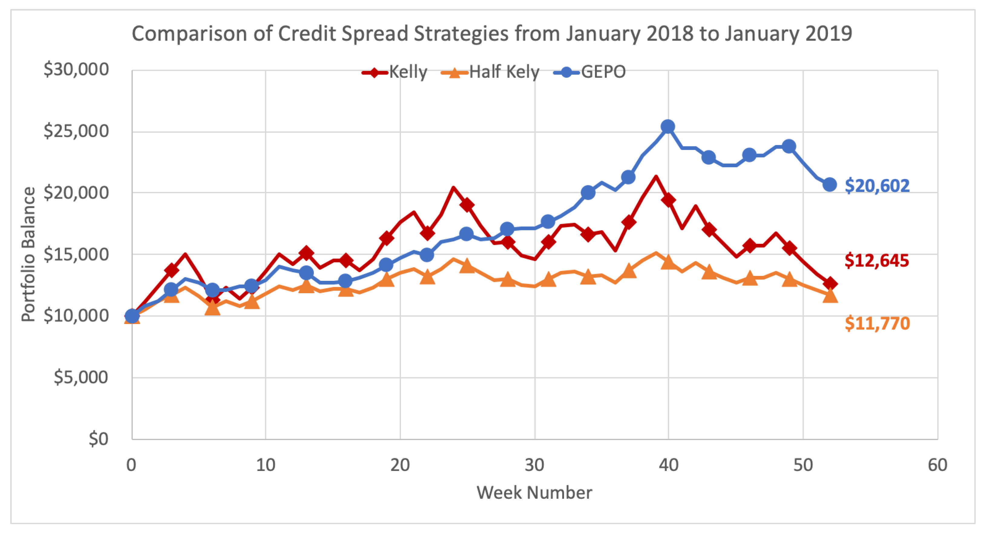
5.3. Comparison to the Kelly Criterion Over Time
6. Conclusions
7. Materials and Methods
Author Contributions
Funding
Conflicts of Interest
Abbreviations
| ADP | Approximate dynamic programming |
| AIG | American International Group |
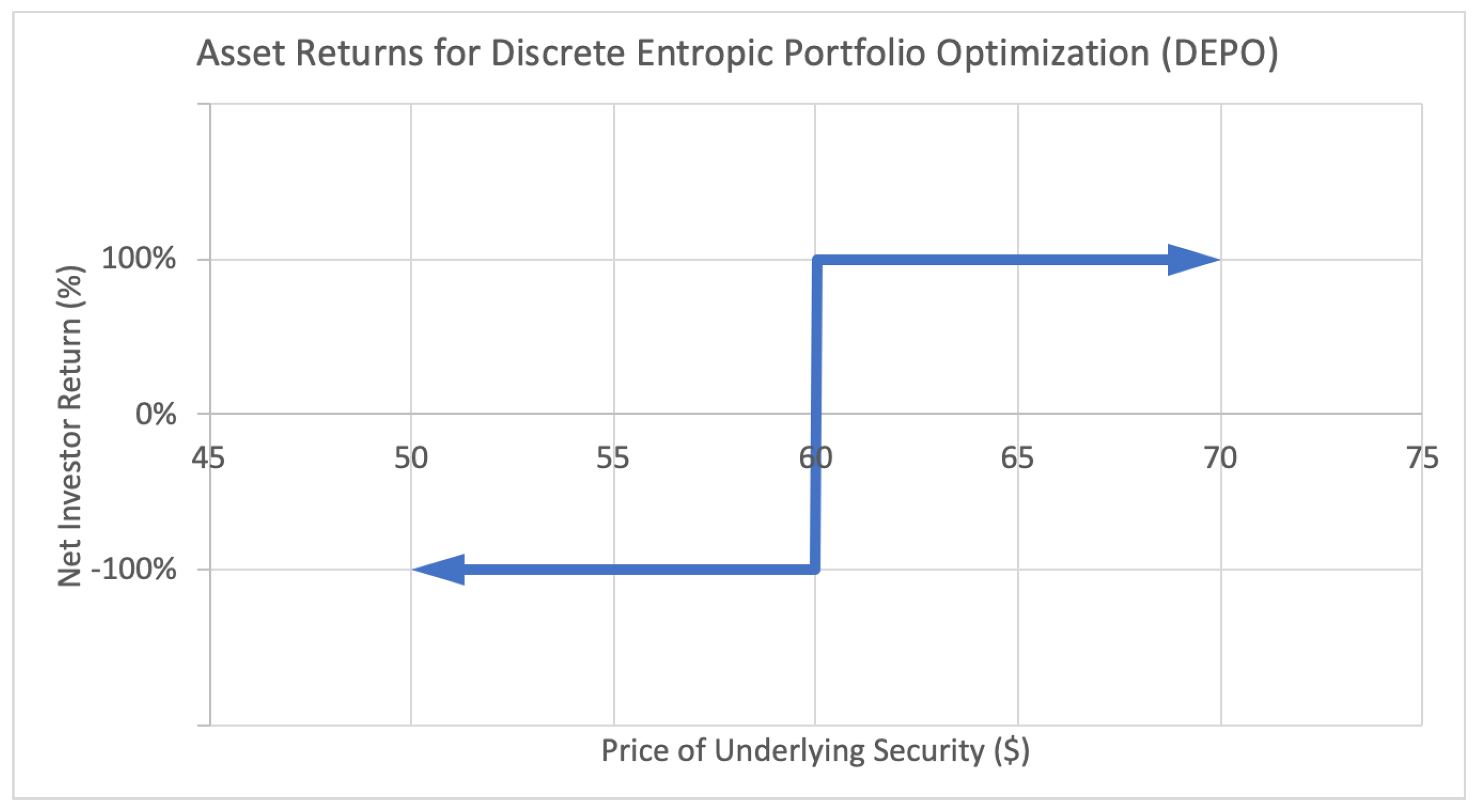
| DEPO | Discrete entropic portfolio optimization |
| FB | Facebook Inc. |
| GEPO | Generalized entropic portfolio optimization |
| IBM | International Business Machines |
| KL | Kullback–Leibler |
| MCD | McDonald’s Corp |
| MRK | Merck & Co. |
| ORCL | Oracle Corp |
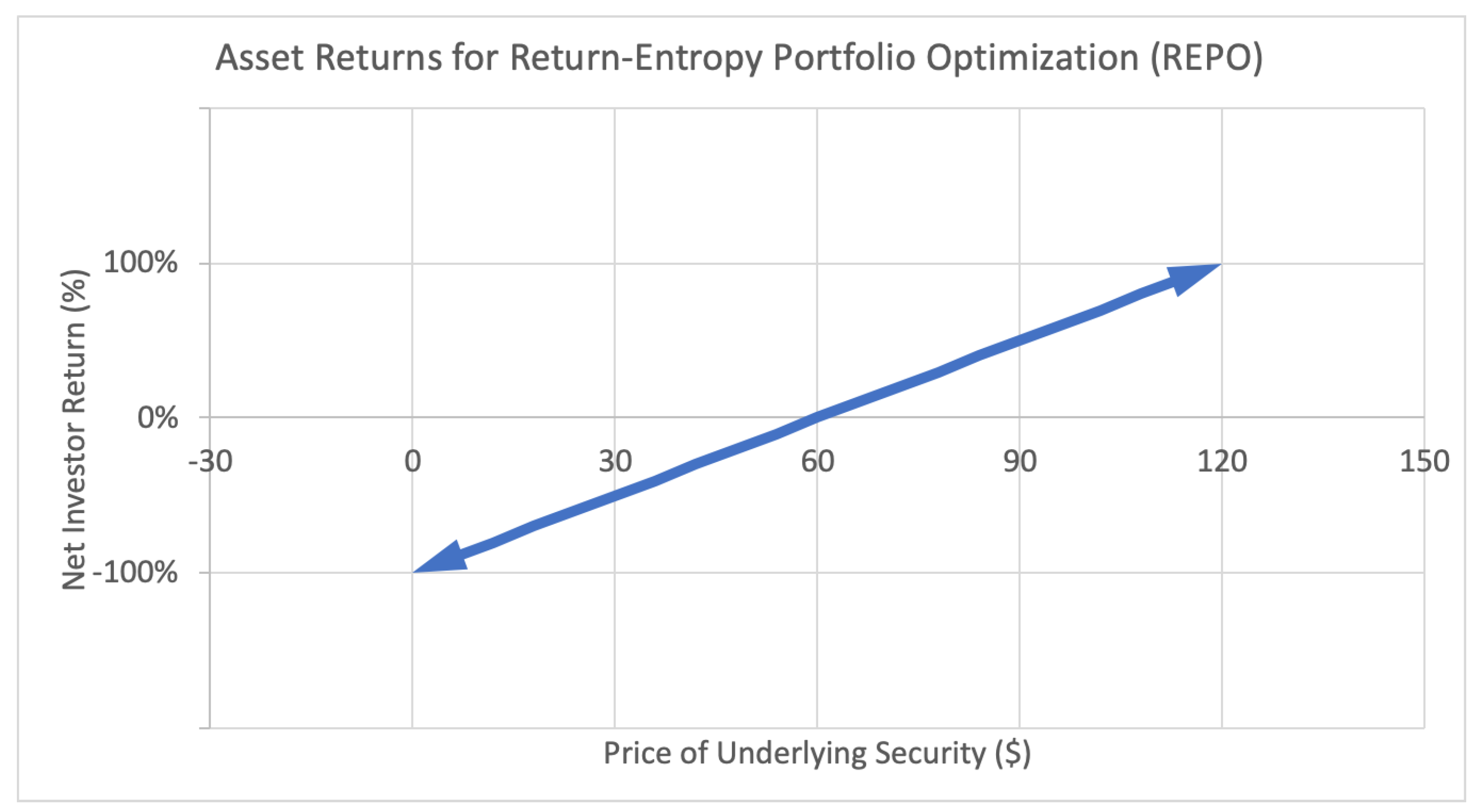
| REPO | Return-entropy portfolio optimization |
| WRDS | Wharton Research Data Services |
References
- Mercurio, P.; Wu, Y.; Xie, H. An Entropy-Based Approach to Portfolio Optimization. Entropy 2020, 22, 332. [Google Scholar] [CrossRef]
- Mercurio, P.; Wu, Y.; Xie, H. Portfolio Optimization for Binary Options Based on Relative Entropy. Entropy 2020, 22, 752. [Google Scholar] [CrossRef]
- Markowitz, H. Portfolio Selection. J. Financ. 1952, 7, 77–91. [Google Scholar]
- Liu, J.; Pan, J. Dynamic Derivative Strategies. J. Financ. Econ. 2003, 69, 401–430. [Google Scholar] [CrossRef]
- Jones, C. A Nonlinear Factor Analysis of S&P 500 Index Option Returns. J. Financ. 2006, 61, 2325–2363. [Google Scholar]
- Eraker, B. The Performance of Model Based Option Trading Strategies. Rev. Deriv. Res. 2007, 16, 1–23. [Google Scholar] [CrossRef]
- Haugh, M.; Kogan, L. Duality Theory and Approximate Dynamic Programming for Pricing American Options and Portfolio Optimization. Handb. Oper. Res. Manag. Sci. 2007, 15, 925–948. [Google Scholar]
- Zymler, S.; Rustem, B.; Kuhn, D. Robust Portfolio Optimization with Derivative Insurance Guarantees. Eur. J. Oper. Res. 2011, 210, 410–424. [Google Scholar] [CrossRef]
- Alexander, S.; Coleman, T.; Li, Y. Derivative Portfolio Hedging Based on CVaR. 2003. Available online: http://citeseerx.ist.psu.edu/viewdoc/download?doi=10.1.1.702.6360&rep=rep1&type=pdf (accessed on 1 July 2020).
- Alexander, S.; Coleman, T.; Li, Y. Minimizing CVaR and VaR for a Portfolio of Derivatives. J. Bank. Financ. 2006, 30, 583–605. [Google Scholar] [CrossRef]
- Zymler, S.; Rustem, B.; Kuhn, D. Worst-Case Value-at-Risk of Non-Linear Portfolios. Manag. Sci. 2013, 59, 172–188. [Google Scholar] [CrossRef]
- Maasar, M.; Roman, D.; Date, P. Portfolio Optimisation Using Risky Assets with Options as Derivative Insurance. In Proceedings of the 5th Student Conference on Operational Research (SCOR 2016), Nottingham, UK, 8–10 April 2016; Volume 50, pp. 1–17. [Google Scholar]
- Driessen, J.; Maenhout, P. The World Price of Volatility and Jump Risk. J. Bank. Financ. 2013, 37, 518–536. [Google Scholar] [CrossRef]
- Constantinides, G.; Jackwerth, J.; Savov, A. The Puzzle of Index Option Returns. Rev. Asset Pricing Stud. 2013, 3, 229–257. [Google Scholar] [CrossRef]
- Fadugba, S. Performance Measure of Binomial Model for Pricing American and European Options. Appl. Comput. Math. 2014, 3, 18–30. [Google Scholar]
- Fu, J.; Wei, J.; Yang, H. Portfolio Optimization in a Regime-Switching Market with Derivatives. Eur. J. Oper. Res. 2014, 233, 184–192. [Google Scholar] [CrossRef]
- Fatyanova, M.; Semenov, M. Model for Constructing an Options Portfolio with a Certain Payoff Function. In Proceedings of the 3rd International Conference on Information Technology and Nanotechnology, Samara, Russia, 25–27 April 2017; Volume 3, pp. 254–262. [Google Scholar]
- Faias, J.; Santa-Clara, P. Optimal Option Portfolio Strategies: Deepening the Puzzle of Index Option Mispricing. J. Financ. Quant. Anal. 2017, 52, 277–303. [Google Scholar] [CrossRef]
- Zhao, L.; Palomar, D. A Markowitz Portfolio Approach to Options Trading. IEEE Trans. Signal Process. 2018, 66, 4223–4238. [Google Scholar] [CrossRef]
- Zeng, Y.; Klabjan, D. Portfolio Optimization for American Options. J. Comput. Financ. 2018, 22, 37–64. [Google Scholar] [CrossRef]
- Kelly, J. A New Interpretation of Information Rate. Bell Syst. Tech. J. 1956, 35, 917–926. [Google Scholar] [CrossRef]
- TMX Group. Montréal Exchange: Guides and Strategies. 2020. Available online: https://m-x.ca/educ_guides_strat_en.php (accessed on 1 March 2020).
- Shannon, C. A Mathematical Theory of Communication: Part 1. Bell Syst. Tech. J. 1948, 27, 379–423. [Google Scholar] [CrossRef]
- Shannon, C. A Mathematical Theory of Communication: Part 2. Bell Syst. Tech. J. 1948, 27, 623–656. [Google Scholar] [CrossRef]
- Kullback, S.; Leibler, R. On Information and Sufficiency. Ann. Math. Stat. 1951, 22, 79–86. [Google Scholar] [CrossRef]
- Kullback, S. Information Theory and Statistics; John Wiley and Sons: New York, NY, USA, 1959. [Google Scholar]


| Company Name | Symbol | Mean Outcome | p-prob | q-prob | -prob | |
|---|---|---|---|---|---|---|
| Apple Inc. | AAPL | 0.10124 | 52.3% | 42.9% | 4.9% | 0.226675 |
| Accenture | ACN | 0.146462 | 54.3% | 38.1% | 7.7% | 0.183754 |
| American Intl. Group | AIG | 0.121123 | 49.8% | 38.2% | 11.9% | 0.118573 |
| Bank of America Corp | BAC | 0.139333 | 49.6% | 32.6% | 17.8% | 0.071421 |
| Biogen | BIIB | −0.048327 | 51.4% | 46.1% | 2.4% | 0.281129 |
| Caterpillar Inc. | CAT | 0.151175 | 53.7% | 38.5% | 7.8% | 0.180714 |
| Capital One Financial Corp | COF | 0.013458 | 46.6% | 45.3% | 8.1% | 0.16507 |
| Costco Wholesale Corp | COST | 0.177373 | 51.8% | 37.3% | 10.8% | 0.135782 |
| Cisco Systems | CSCO | 0.340769 | 59.6% | 25% | 15.4% | 0.141729 |
| Facebook Inc. | FB | 0.128127 | 53.5% | 42.3% | 4.2% | 0.242447 |
| Intl. Business Machines | IBM | 0.148669 | 53.2% | 38.7% | 8.2% | 0.173439 |
| Intel Corp | INTC | 0.143774 | 51.7% | 35.5% | 12.8% | 0.115093 |
| Johnson & Johnson | JNJ | 0.290017 | 61.9% | 32.6% | 5.5% | 0.251597 |
| JPMorgan Chase & Co. | JPM | 0.223986 | 58% | 36.4% | 5.6% | 0.230925 |
| MasterCard Inc. | MA | 0.125993 | 53.3% | 40.8% | 5.9% | 0.209407 |
| McDonald’s Corp | MCD | 0.160243 | 53% | 37.7% | 9.3% | 0.157863 |
| 3M Company | MMM | 0.18277 | 55.7% | 35.7% | 8.6% | 0.17661 |
| Merck & Co. | MRK | 0.177165 | 54% | 37.9% | 8% | 0.17795 |
| Microsoft | MSFT | 0.170696 | 55.3% | 38.5% | 6.2% | 0.209972 |
| Oracle Corp | ORCL | 0.286192 | 60.1% | 30.6% | 9.3% | 0.191343 |
| Symbol | Spread Type | Spread Interval | Sell Delta | Buy Delta | p-proj | q-proj | -proj |
|---|---|---|---|---|---|---|---|
| AAPL | Put | [167.5, 170] | −0.496757 | −0.405426 | 50.3% | 40.5% | 9.1% |
| ACN | Call | [149, 150] | 0.492771 | 0.447763 | 50.7% | 44.8% | 4.5% |
| AIG | Call | [60, 61] | 0.489573 | 0.345599 | 51% | 34.6% | 14.4% |
| BAC | Put | [28.5, 29] | −0.497381 | −0.401975 | 50.3% | 40.2% | 9.5% |
| BIIB | Put | [317.5, 320] | −0.495617 | −0.448496 | 50.4% | 44.8% | 4.7% |
| CAT | Put | [149, 150] | −0.497975 | −0.43738 | 50.2% | 43.7% | 6.1% |
| COF | Call | [92.5, 93] | 0.498336 | 0.465034 | 50.2% | 46.5% | 3.3% |
| COST | Put | [182.5, 185] | −0.497485 | −0.417452 | 50.3% | 41.7% | 8% |
| CSCO | Put | [36.5, 37] | −0.496195 | −0.374409 | 50.4% | 37.4% | 12.2% |
| FB | Put | [170, 172.5] | −0.487722 | −0.392952 | 51.2% | 39.3% | 9.5% |
| IBM | Put | [150, 152.5] | −0.494561 | −0.311505 | 50.5% | 31.2% | 18.3% |
| INTC | Put | [44, 44.5] | −0.496887 | −0.403415 | 50.3% | 40.3% | 9.3% |
| JNJ | Call | [142, 143] | 0.499681 | 0.408484 | 50% | 40.8% | 9.1% |
| JPM | Call | [105, 106] | 0.499166 | 0.435065 | 50.1% | 43.5% | 6.4% |
| MA | Call | [146, 147] | 0.494829 | 0.433672 | 50.5% | 43.4% | 6.1% |
| MCD | Put | [170, 172.5] | −0.499101 | −0.335054 | 50.1% | 33.5% | 16.4% |
| MMM | Call | [242.5, 245] | 0.495376 | 0.398127 | 50.5% | 39.8% | 9.7% |
| MRK | Call | [55, 55.5] | 0.48691 | 0.405147 | 51.3% | 40.5% | 8.2% |
| MSFT | Call | [84.5, 85] | 0.498834 | 0.451614 | 50.1% | 45.2% | 4.7% |
| ORCL | Call | [50, 51] | 0.490397 | 0.374001 | 51% | 37.4% | 11.6% |
| Symbol | Spread Type | Spread Interval | p-proj | q-proj | -proj | Kelly Allocation % |
|---|---|---|---|---|---|---|
| IBM | Put | [150, 152.5] | 50.5% | 31.2% | 18.3% | 12% |
| Symbol | Spread Type | Spread Interval | p-proj | q-proj | -proj | GEPO Allocation % |
|---|---|---|---|---|---|---|
| IBM | Put | [150, 152.5] | 50.5% | 31.2% | 18.3% | 1.5% |
| AIG | Call | [60, 61] | 51% | 34.6% | 14.1% | 1.5% |
| MCD | Put | [170, 172.5] | 50.1% | 33.5% | 16.4% | 1.5% |
| ORCL | Call | [50, 51] | 51% | 37.4% | 11.6% | 1.5% |
| FB | Put | [170, 172.5] | 51.2% | 39.3% | 9.5% | 1.5% |
| MRK | Call | [55, 55.5] | 51.3% | 40.5% | 8.2% | 1.5% |
© 2020 by the authors. Licensee MDPI, Basel, Switzerland. This article is an open access article distributed under the terms and conditions of the Creative Commons Attribution (CC BY) license (http://creativecommons.org/licenses/by/4.0/).
Share and Cite
Mercurio, P.J.; Wu, Y.; Xie, H. Option Portfolio Selection with Generalized Entropic Portfolio Optimization. Entropy 2020, 22, 805. https://doi.org/10.3390/e22080805
Mercurio PJ, Wu Y, Xie H. Option Portfolio Selection with Generalized Entropic Portfolio Optimization. Entropy. 2020; 22(8):805. https://doi.org/10.3390/e22080805
Chicago/Turabian StyleMercurio, Peter Joseph, Yuehua Wu, and Hong Xie. 2020. "Option Portfolio Selection with Generalized Entropic Portfolio Optimization" Entropy 22, no. 8: 805. https://doi.org/10.3390/e22080805
APA StyleMercurio, P. J., Wu, Y., & Xie, H. (2020). Option Portfolio Selection with Generalized Entropic Portfolio Optimization. Entropy, 22(8), 805. https://doi.org/10.3390/e22080805