Calculating the Wasserstein Metric-Based Boltzmann Entropy of a Landscape Mosaic


Abstract
1. Introduction
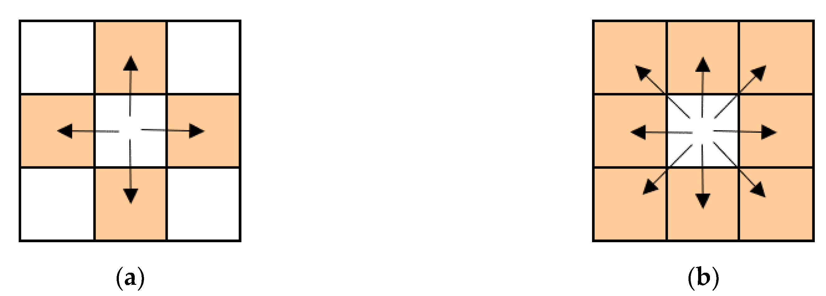
2. Wasserstein Metric-Based Boltzmann Entropy
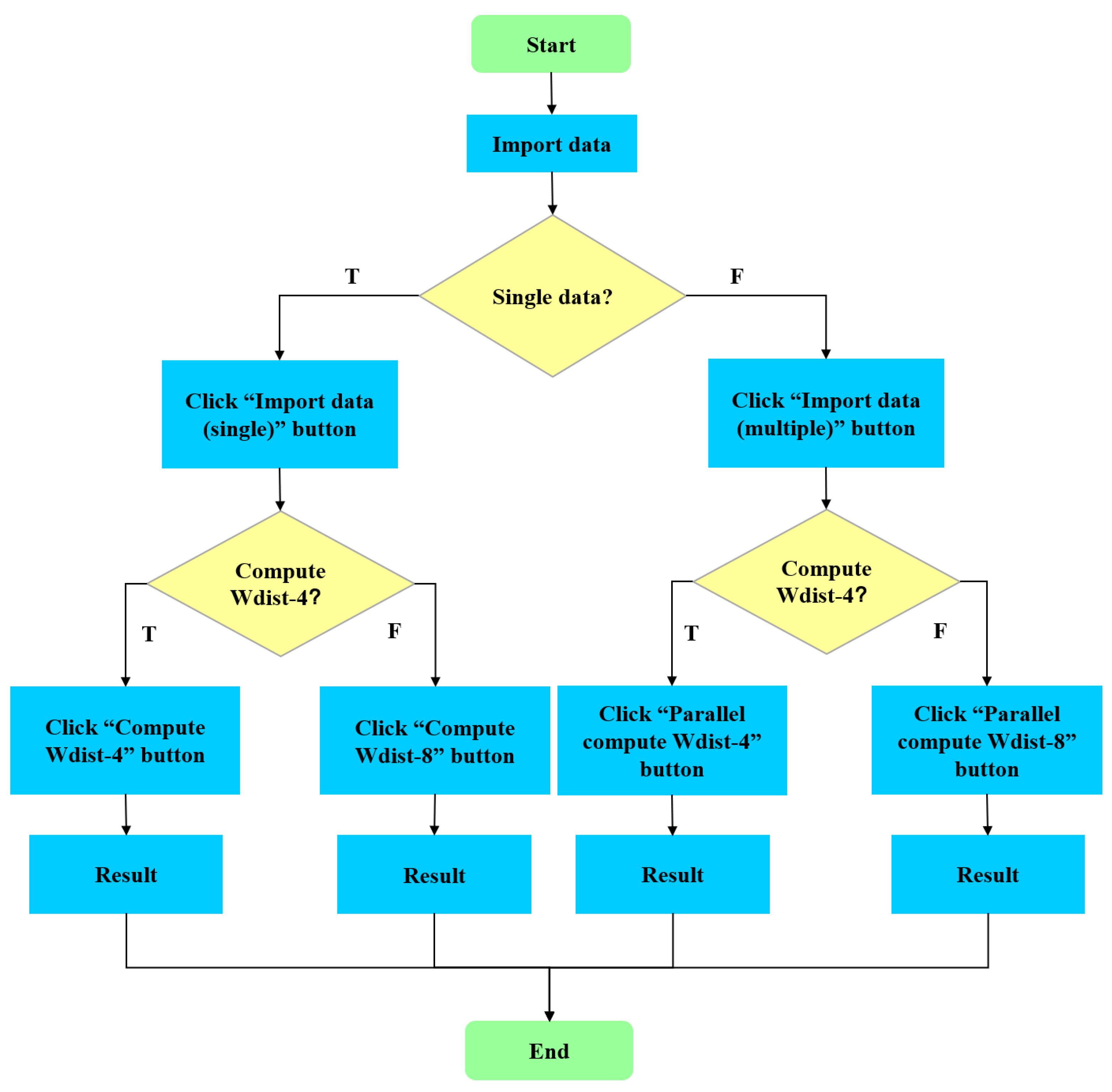
3. Design of a Software Tool for Conveniently Calculating
4. Technical Implementation of the Software Tool
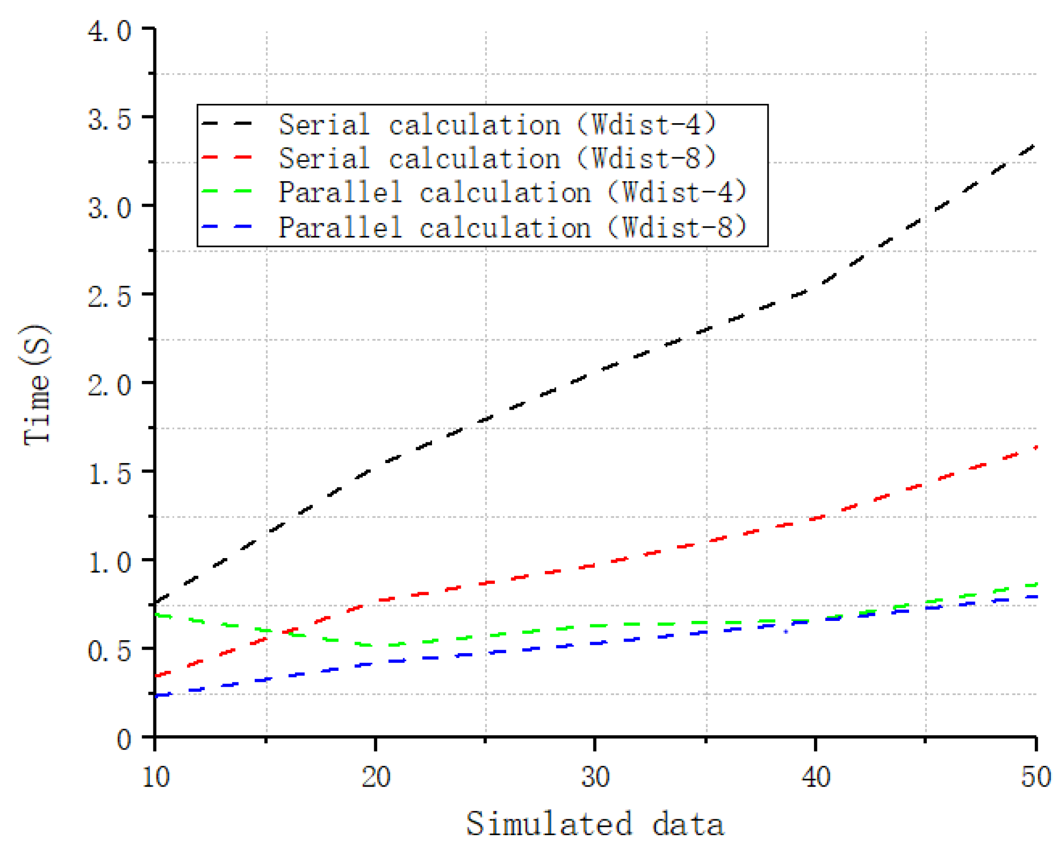
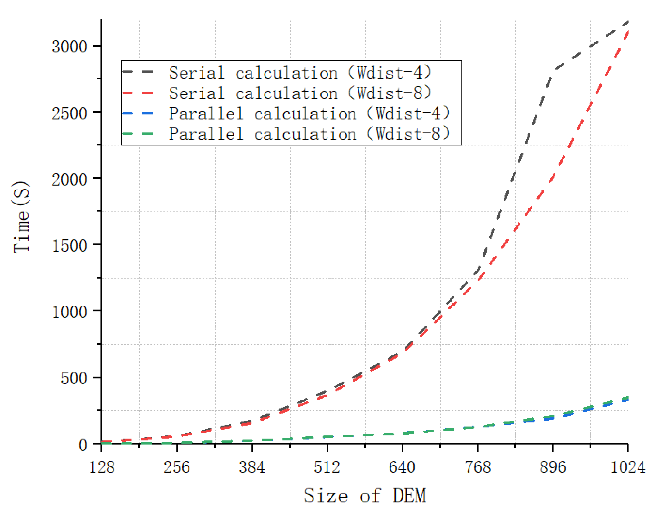
5. Evaluation
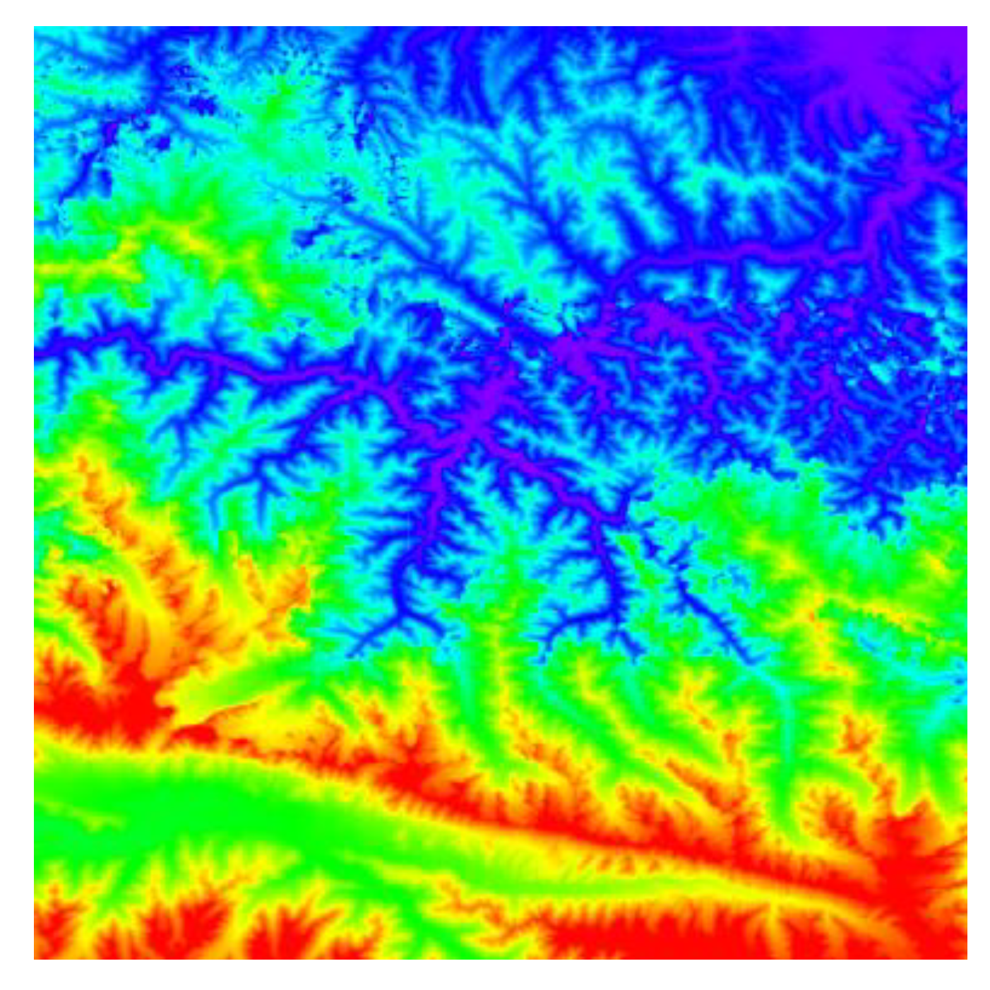
6. Case Studies
7. Discussion
8. Concluding Remarks
Supplementary Materials
Author Contributions
Funding
Acknowledgments
Conflicts of Interest
References
- Paszto, V.; Brychtová, A.; Tuček, P.; Marek, L.; Burian, J. Using a fuzzy inference system to delimit rural and urban municipalities in the Czech republic in 2010. J. Maps 2015, 11, 231–239. [Google Scholar] [CrossRef]
- Pászto, V.; Brychtová, A.; Marek, L. On shape metrics in cartographic generalization: A case study of the building footprint geometry. In Modern Trends in Cartography; Springer: Berlin/Heidelberg, Germany, 2015; pp. 397–407. [Google Scholar]
- LI, Z.L.; Gong, X.Y.; Chen, J.; Mills, J.; Li, S.N.; Zhu, X.; Ti, P.; Wu, H. Functional Requirements of Systems for Visualization of Sustainable Development Goal (SDG) Indicators. J. Geovis. Spat. Anal. 2020, 4, 1–10. [Google Scholar]
- Zhang, J.; Zhou, Q.; Shen, X.; Li, Y.S. Cloud detection in high-resolution remote sensing images using multi-features of ground objects. J. Geovis. Spat. Anal. 2019, 3, 14. [Google Scholar] [CrossRef]
- Frick, A.; Tervooren, S. A framework for the long-term monitoring of urban green volume based on multi-temporal and multi-sensoral remote sensing data. J. Geovis. Spat. Anal. 2019, 3, 6. [Google Scholar] [CrossRef]
- Jiang, B.; Ma, D. How complex is a fractal? Head/tail breaks and fractional hierarchy. J. Geovis. Spat. Anal. 2018, 2, 6. [Google Scholar] [CrossRef]
- Pászto, V. Economic Geography. In Spationomy: Spatial Exploration of Economic Data and Methods of Interdisciplinary Analytics; Pászto, V., Jürgens, C., Tominc, P., Burian, J., Eds.; Springer International Publishing: Cham, Switzerland, 2020; pp. 173–192. [Google Scholar] [CrossRef]
- Jiang, B.; Ren, Z. Geographic space as a living structure for predicting human activities using big data. Int. J. Geogr. Inf. Sci. 2019, 33, 764–779. [Google Scholar] [CrossRef]
- Sun, W.W.; Du, Q. Graph-regularized fast and robust principal component analysis for hyperspectral band selection. IEEE Trans. Geosci. Remote Sens. 2018, 56, 3185–3195. [Google Scholar] [CrossRef]
- Gao, P.C.; Cushman, S.A.; Liu, G.; Ye, S.J.; Shen, S.; Cheng, C.X. FracL: A tool for characterizing the fractality of landscape gradients from a new perspective. ISPRS Int. J. Geo-Inf. 2019, 8, 466. [Google Scholar] [CrossRef]
- Liew, A. Understanding data, information, knowledge and their inter-relationships. J. Knowl. Manag. Pract. 2007, 8, 1–16. [Google Scholar]
- Liu, J.; Huang, J.Y.; Liu, S.G.; Li, H.L.; Zhou, Q.M.; Liu, J.C. Human visual system consistent quality assessment for remote sensing image fusion. Int. J. Photogr. Remote Sens. 2015, 105, 79–90. [Google Scholar] [CrossRef]
- Li, S.; Li, Z.L.; Gong, J.Y. Multivariate statistical analysis of measures for assessing the quality of image fusion. Int. J. Image Data Fusion 2010, 1, 47–66. [Google Scholar] [CrossRef]
- Sun, W.W.; Yang, G.; Wu, K.; Li, W.Y.; Zhang, D.F. Pure endmember extraction using robust kernel archetypoid analysis for hyperspectral imagery. Int. J. Photogr. Remote Sens. 2017, 131, 147–159. [Google Scholar] [CrossRef]
- Gao, P.C.; Wang, J.C.; Zhang, H.; Li, Z.L. Boltzmann entropy-based unsupervised band selection for hyperspectral image classification. IEEE Geosci. Remote Sens. Lett. 2019, 16, 462–466. [Google Scholar] [CrossRef]
- McGarigal, K.; Tagil, S.; Cushman, S.A. Surface metrics: An alternative to patch metrics for the quantification of landscape structure. Landsc. Ecol. 2009, 24, 433–450. [Google Scholar] [CrossRef]
- Gustafson, E.J. How has the state-of-the-art for quantification of landscape pattern advanced in the twenty-first century? Landsc. Ecol. 2019, 34, 2065–2072. [Google Scholar] [CrossRef]
- Shannon, C.E.; Weaver, W. The Mathematical Theory of Communication; The University of Illinois Press: Urbana, IL, USA, 1949. [Google Scholar]
- Shannon, C.E. A mathematical theory of communication. Bell Syst. Tech. J. 1948, 27, 379–423. [Google Scholar] [CrossRef]
- Nowosad, J.; Stepinski, T.F. Information theory as a consistent framework for quantification and classification of landscape patterns. Landsc. Ecol. 2019, 34, 2091–2101. [Google Scholar] [CrossRef]
- Fan, Y.; Yu, G.M.; He, Z.Y.; Yu, H.L.; Bai, R.; Yang, L.R.; Wu, D. Entropies of the Chinese land use/cover change from 1990 to 2010 at a county level. Entropy 2017, 19, 51. [Google Scholar] [CrossRef]
- Hu, L.J.; He, Z.Y.; Liu, J.P.; Zheng, C.H. Method for measuring the information content of terrain from digital elevation models. Entropy 2015, 17, 7021–7051. [Google Scholar] [CrossRef]
- Batty, M. Spatial entropy. Geogr. Anal. 1974, 6, 1–31. [Google Scholar] [CrossRef]
- Batty, M.; Morphet, R.; Masucci, P.; Stanilov, K. Entropy, complexity, and spatial information. J. Geogr. Syst. 2014, 16, 363–385. [Google Scholar] [CrossRef] [PubMed]
- Wilson, A. Entropy in urban and regional modelling: Retrospect and prospect. Geogr. Anal. 2010, 42, 364–394. [Google Scholar] [CrossRef]
- Zhang, J.X.; Atkinson, P.M.; Goodchild, M.F. Scale in Spatial Information and Analysis; CRC Press: Boca Raton, FL, USA, 2014. [Google Scholar]
- Wise, S. Information entropy as a measure of DEM quality. Comput. Geosci. 2012, 48, 102–110. [Google Scholar] [CrossRef]
- Altieri, L.; Cocchi, D.; Roli, G. A new approach to spatial entropy measures. Environ. Ecol. Stat. 2018, 25, 95–110. [Google Scholar] [CrossRef]
- Li, Z.L.; Huang, P.Z. Quantitative measures for spatial information of maps. Int. J. Geogr. Inf. Sci. 2002, 16, 699–709. [Google Scholar] [CrossRef]
- Zhang, T.; Cheng, C.; Gao, P. Permutation entropy-based analysis of temperature complexity spatial-temporal variation and its driving factors in China. Entropy 2019, 21, 1001. [Google Scholar] [CrossRef]
- Wang, C.J.; Zhao, H.R. Spatial heterogeneity analysis: Introducing a new form of spatial entropy. Entropy 2018, 20, 398. [Google Scholar] [CrossRef]
- Gao, P.C.; Li, Z.L.; Zhang, H. Thermodynamics-based evaluation of various improved Shannon entropies for configurational information of gray-level images. Entropy 2018, 20, 19. [Google Scholar] [CrossRef]
- Cushman, S.A. Thermodynamics in landscape ecology: The importance of integrating measurement and modeling of landscape entropy. Landsc. Ecol. 2015, 30, 7–10. [Google Scholar] [CrossRef]
- Cushman, S.A. Editorial: Entropy in landscape ecology. Entropy 2018, 20, 314. [Google Scholar] [CrossRef]
- Vranken, I.; Baudry, J.; Aubinet, M.; Visser, M.; Bogaert, J. A review on the use of entropy in landscape ecology: Heterogeneity, unpredictability, scale dependence and their links with thermodynamics. Landsc. Ecol. 2015, 30, 51–65. [Google Scholar] [CrossRef]
- Pelorosso, R.; Gobattoni, F.; Leone, A. The low-entropy city: A thermodynamic approach to reconnect urban systems with nature. Landsc. Urban Plan. 2017, 168, 22–30. [Google Scholar] [CrossRef]
- Wilson, A. The “thermodynamics” of the city. In Complexity and Spatial Networks; Reggiani, A., Nijkamp, P., Eds.; Springer: Dordrecht, The Netherlands, 2009; pp. 11–31. [Google Scholar]
- Sugihakim, R.; Alatas, H. Application of a Boltzmann-entropy-like concept in an agent-based multilane traffic model. Phys. Lett. A 2016, 380, 147–155. [Google Scholar] [CrossRef]
- Cushman, S.A. Calculating the configurational entropy of a landscape mosaic. Landsc. Ecol. 2016, 31, 481–489. [Google Scholar] [CrossRef]
- Boltzmann, L. Weitere Studien über das Wärmegleichgewicht unter Gasmolekülen [Further studies on the thermal equilibrium of gas molecules]. Sitz. Akad. Wiss. 1872, 66, 275–370. [Google Scholar]
- Gokcen, N.A.; Reddy, R.G. Thermodynamics; Springer: New York, NY, USA, 2013. [Google Scholar]
- Dalarsson, N.; Dalarsson, M.; Golubovic, L. Introductory Statistical Thermodynamics; Academic Press: Amsterdam, The Netherlands, 2011. [Google Scholar]
- Cushman, S.A. Calculation of configurational entropy in complex landscapes. Entropy 2018, 20, 298. [Google Scholar] [CrossRef]
- Gao, P.C.; Li, Z.L. Computation of the Boltzmann entropy of a landscape: A review and a generalization. Landsc. Ecol. 2019, 34, 2183–2196. [Google Scholar] [CrossRef]
- Gao, P.C.; Li, Z.L. Aggregation-based method for computing absolute Boltzmann entropy of landscape gradient with full thermodynamic consistency. Landsc. Ecol. 2019, 34, 1837–1847. [Google Scholar] [CrossRef]
- Gao, P.C.; Zhang, H.; Li, Z.L. A hierarchy-based solution to calculate the configurational entropy of landscape gradients. Landsc. Ecol. 2017, 32, 1133–1146. [Google Scholar] [CrossRef]
- Zhao, Y.; Zhang, X.C. Calculating spatial configurational entropy of a landscape mosaic based on the Wasserstein metric. Landsc. Ecol. 2019, 34, 1849–1858. [Google Scholar] [CrossRef]
- Nowosad, J. Belg: Boltzmann Entropy of a Landscape Gradient. R Package Version 0.2.3. Available online: https://CRAN.R-project.org/package=belg (accessed on 29 January 2020).
- Forman, R.T.T. Land Mosaics: The Ecology of Landscapes and Regions; Cambridge University Press: Cambridge, UK, 1995. [Google Scholar]
- McGarigal, K.; Cushman, S.A. The gradient concept of landscape structure. In Issues and Perspectives in Landscape Ecology; Wiens, J.A., Moss, M.R., Eds.; Cambridge University Press: Cambridge, UK, 2005; pp. 112–119. [Google Scholar] [CrossRef]
- Evans, J.S.; Cushman, S.A. Gradient modeling of conifer species using random forests. Landsc. Ecol. 2009, 24, 673–683. [Google Scholar] [CrossRef]
- Gulrajani, I.; Ahmed, F.; Arjovsky, M.; Dumoulin, V.; Courville, A.C. Improved training of wasserstein gans. In Proceedings of the Advances in Neural Information Processing Systems, Long Beach, CA, USA, 4–9 December 2017; pp. 5767–5777. [Google Scholar]
- Frazier, A.E. Emerging trajectories for spatial pattern analysis in landscape ecology. Landsc. Ecol. 2019, 34, 2073–2082. [Google Scholar] [CrossRef]
- Kedron, P.J.; Frazier, A.E.; Ovando-Montejo, G.A.; Wang, J. Surface metrics for landscape ecology: A comparison of landscape models across ecoregions and scales. Landsc. Ecol. 2018, 33, 1489–1504. [Google Scholar] [CrossRef]
- Lv, Z.Y.; Zhang, P.; Atli Benediktsson, J. Automatic object-oriented, spectral-spatial feature extraction driven by Tobler’s First Law of Geography for very high resolution aerial imagery classification. Remote Sens. 2017, 9, 285. [Google Scholar] [CrossRef]
- Wang, L.; Shi, C.; Diao, C.Y.; Ji, W.J.; Yin, D.M. A survey of methods incorporating spatial information in image classification and spectral unmixing. Int. J. Remote Sens. 2016, 37, 3870–3910. [Google Scholar] [CrossRef]
- Gao, P.C.; Liu, Z.; Han, F.; Tang, L.; Xie, M.H. Accelerating the computation of multi-scale visual curvature for simplifying a large set of polylines with Hadoop. Gisci. Remote Sens. 2015, 52, 315–331. [Google Scholar] [CrossRef]
- Qin, C.Z.; Zhan, L.J.; Zhu, A.X. How to apply the Geospatial Data Abstraction Library (GDAL) properly to parallel geospatial raster I/O? Trans. GIS 2014, 18, 950–957. [Google Scholar] [CrossRef]
- Qin, C.Z.; Zhan, L.J.; Zhu, A.X.; Zhou, C.H. A strategy for raster-based geocomputation under different parallel computing platforms. Int. J. Geogr. Inf. Sci. 2014, 28, 2127–2144. [Google Scholar] [CrossRef]
- Gao, P.C.; Liu, Z.; Xie, M.H.; Tian, K. Low-cost cloud computing solution for geo-information processing. J. Cent. South Univ. 2016, 23, 3217–3224. [Google Scholar] [CrossRef]
- Gardner, R.H. RULE: Map generation and a spatial analysis program. In Landscape Ecological Analysis: Issues and Applications; Klopatek, J.M., Gardner, R.H., Eds.; Springer: New York, NY, USA, 1999; pp. 280–303. [Google Scholar]
- Razakarivony, S.; Jurie, F. Vehicle detection in aerial imagery: A small target detection benchmark. J. Vis. Commun. Image Represent. 2016, 34, 187–203. [Google Scholar] [CrossRef]
- Xu, J.Y.; Liang, X.Y.; Chen, H. Landscape sustainability evaluation of ecologically fragile areas based on Boltzmann entropy. ISPRS Int. J. Geo-Inf. 2020, 9, 77. [Google Scholar] [CrossRef]


| Landscape | ||
|---|---|---|
| a | 0.1611 | 0.1294 |
| b | 0.1345 | 0.1006 |
| c | 0.0829 | 0.0688 |
| d | 0.0601 | 0.0590 |
| Dissimilarity | ||
|---|---|---|
| Images 0 and 1 | ||
| Images 0 and 2 | ||
| Images 0 and 3 | ||
| Images 0 and 4 |
| Data | ||||
|---|---|---|---|---|
| Landscape a | 0.8054 | 0.8054 | 0.1720 | 0.3352 |
| Landscape b | 0.8055 | 0.8055 | 0.3086 | 0.4827 |
| Landscape c | 0.8057 | 0.8057 | 0.5735 | 0.6461 |
| Landscape d | 0.8058 | 0.8058 | 0.6905 | 0.6960 |
| Image 0 | 0.6633 | 0.6633 | 0.0256 | 0.0396 |
| Image 1 | 0.6633 | 0.6633 | 0.0221 | 0.0330 |
| Image 2 | 0.6633 | 0.6633 | 0.0178 | 0.0246 |
| Image 3 | 0.6633 | 0.6633 | 0.0150 | 0.0192 |
| Image 4 | 0.6633 | 0.6633 | 0.0128 | 0.0146 |
© 2020 by the authors. Licensee MDPI, Basel, Switzerland. This article is an open access article distributed under the terms and conditions of the Creative Commons Attribution (CC BY) license (http://creativecommons.org/licenses/by/4.0/).
Share and Cite
Zhang, H.; Wu, Z.; Lan, T.; Chen, Y.; Gao, P. Calculating the Wasserstein Metric-Based Boltzmann Entropy of a Landscape Mosaic. Entropy 2020, 22, 381. https://doi.org/10.3390/e22040381
Zhang H, Wu Z, Lan T, Chen Y, Gao P. Calculating the Wasserstein Metric-Based Boltzmann Entropy of a Landscape Mosaic. Entropy. 2020; 22(4):381. https://doi.org/10.3390/e22040381
Chicago/Turabian StyleZhang, Hong, Zhiwei Wu, Tian Lan, Yanyu Chen, and Peichao Gao. 2020. "Calculating the Wasserstein Metric-Based Boltzmann Entropy of a Landscape Mosaic" Entropy 22, no. 4: 381. https://doi.org/10.3390/e22040381
APA StyleZhang, H., Wu, Z., Lan, T., Chen, Y., & Gao, P. (2020). Calculating the Wasserstein Metric-Based Boltzmann Entropy of a Landscape Mosaic. Entropy, 22(4), 381. https://doi.org/10.3390/e22040381