Abstract
In this survey we stress the importance of the higher transcendental Mittag-Leffler function in the framework of the Fractional Calculus. We first start with the analytical properties of the classical Mittag-Leffler function as derived from being the solution of the simplest fractional differential equation governing relaxation processes. Through the sections of the text we plan to address the reader in this pathway towards the main applications of the Mittag-Leffler function that has induced us in the past to define it as the Queen Function of the Fractional Calculus. These applications concern some noteworthy stochastic processes and the time fractional diffusion-wave equation We expect that in the future this function will gain more credit in the science of complex systems. Finally, in an appendix we sketch some historical aspects related to the author’s acquaintance with this function.
1. Introduction
For few decades, the special transcendental function known as the Mittag-Leffler function has attracted increasing attention of researchers because of its key role in treating problems related to integral and differential equations of fractional order.
His function was introduced in 1903–1905 by the Swedish mathematician Mittag-Leffler and at the beginning of the last century up to the 1990s, this function was seldom considered by mathematicians and applied scientists.
Before the 1990s, from a mathematical point of view, we recall the 1930 paper by Hille and Tamarkin [1] on the solutions of the Abel integral equation of the second kind, and the books by Davis [2], Sansone & Gerretsen [3], Dzherbashyan [4] (unfortunately in Russian), and finally Samko et al. [5]. Particular mention would be for the 1955 Handbook of High Transcendental Functions of the Bateman project [6], where this function was treated in Volume 3, in the chapter devoted to miscellaneous functions. For former applications we recall an interesting note by Davis [2] reporting previous research by Dr. Kenneth S. Cole in connection with nerve conduction, and the papers by Cole & Cole [7], Gross [8] and Caputo & Mainardi [9,10], where the Mittag-Leffler function was adopted to represent the responses in dielectric and viscoelastic media. More information are found in the Appendix of this survey.
In the 1960’s the Mittag-Leffler function started to emerge from the realm of miscellaneous functions because it was considered as a special case of the general class of Fox H functions, that can exhibit an arbitrary number of parameters in their integral Mellin-Barnes representation. However, in our opinion, this classification in a too general framework has, to some extent, obscured the relevance and the applicability of this function in applied sciences. In fact, most mathematical models are based on a small number of parameters, say 1 or 2 or 3, so that a general theory may be confusing whereas the adoption of a generalized Mittag-Leffler function with 2 or 3 indices may be sufficient.
Nowadays it is well recognized that the Mittag-Leffler function plays a fundamental role in Fractional Calculus even if with a single parameter (as originally introduced by Mittag-Leffler) just to be worthy of being referred to as the Queen Function of Fractional Calculus, see Mainardi & Gorenflo [11]. We find some information on the Mittag-Leffler functions in any treatise on Fractional Calculus but for more details we refer the reader to the surveys of Haubold, Mathai and Saxena [12] and by Van Mieghem [13] and to the treatise by Gorenflo et al. [14], devoted just to Mittag-Leffler functions, related topics and applications.
The plan of this survey is the following. We start to give in Section 2 the main definitions and properties of the Mittag-Leffler function in one parameter with related Laplace transforms. Then in Section 3 we describe its use in the simplest fractional relaxation equation pointing out its compete monotonicity. The asymptotic properties are briefly discussed in Section 4. In Section 5 we briefly discuss the so called generalized Mittag-Leffler function, that is the 2-parameter Mittag-Leffler function. Of course further generalization to 3 and more parameter will be referred to specialized papers and books. Then in the following sections we discuss the application of the Mittag-Leffler function in some noteworthy stochastic processes. We start in Section 6 with the fractional Poisson process, and then in Section 7 with its application of the thinning of renewal processes. The main application are dealt in Section 8 where we discuss the continuous time random walks (CTRW) and then in Section 9 we point out the asymptotic universality. In Section 10 we discuss the time fractional diffusion-wave processes pointing out the role of the Mittag-Leffler functions in two parameters and their connection with the basic Wright functions. In Appendix A we find it worthwhile to report the acquaintance of the author with the Mittag-Leffler functions started in the late 1960s and continued up to nowadays.
We recall that Section 3, Section 4, Section 5, Section 6, Section 7, Section 8, Section 9 and Section 10 are taken from several papers by the author, published alone and with colleagues and former students. Furthermore we have not considered other applications of the Mittag-Leffler functions including, for example, anomalous diffusion theory in terms of fractional and generalized Langevin equations. On this respect we refer the readers to the articles of the author, see References [15,16], and to the recent book by Sandev and Tomovski [17] and references therein. For many items related to the Mittag-Leffler functions we refer again to the treatise by Gorenflo et al. [14].
2. The Mittag-Leffler Functions: Definitions and Laplace Transforms
The Mittag-Leffler function is defined by the following power series, convergent in the whole complex plane,
We recognize that it is an entire function of order providing a simple generalization of the exponential function to which it reduces for . For detailed information on the Mittag-Leffler-type functions and their Laplace transforms the reader may consult e.g., [6,18,19] and the recent treatise by Gorenflo et al. [14].
We also note that for the convergence of the power series in (1) the parameter may be complex provided that . The most interesting properties of the Mittag-Leffler function are associated with its asymptotic expansions as in various sectors of the complex plane.
In this paper we mainly consider the Mittag-Leffler function of order on the negative real semi-axis where is known to be completely monotone (CM) due a classical result by Pollard [20], see also Feller [21].
Let us recall that a function with is called a completely monotone (CM) function if it is non-negative, of class , and for all . Then a function with is called a Bernstein function if it is non-negative, of class , with a CM first derivative. These functions play fundamental roles in linear hereditary mechanics to represent relaxation and creep processes, see, for example, Mainardi [22]. For mathematical details we refer the interested reader to the survey paper by Miller and Samko [23] and to the treatise by Schilling et al. [24].
In particular we are interested in the function
whose Laplace transform pair reads
Here we have used the notation ÷ to denote the juxtaposition of a function of time with its Laplace transform
The pair (3) can be proved by transforming term by term the power series representation of in the R.H.S of (2). Similarly we can prove the following Laplace transform pair for its time derivative
For this Laplace transform pair we can simply apply the usual rule for the Laplace transform for the first derivative of a function, that reads
3. The Mittag-Leffler Function in Fractional Relaxation Processes
For readers’ convenience let us briefly outline the topic concerning the generalization via fractional calculus of the first-order differential equation governing the phenomenon of (exponential) relaxation. Recalling (in non-dimensional units) the initial value problem
whose solution is
the following two alternatives with are offered in the literature:
where and denote the fractional derivative of order in the Riemann-Liouville sense and the fractional derivative of order in the Caputo sense, respectively.
For a generic order and for a sufficiently well-behaved function with the above derivatives are defined as follows, see for example, Gorenflo and Mainardi [18], Podlubny [19],
Between the two derivatives we have the relationship
Both derivatives in the limit reduce to the standard first derivative but for we have
In analogy to the standard problem (5), we solve the problems (7) and (8) with the Laplace transform technique, using the rules pertinent to the corresponding fractional derivatives, that we recall hereafter for a generic order ,
We note that it is generally more cumbersome to use the Laplace transform pair for the Riemann Liouville derivative (13) than for the Capute derivative (14). Indeed the rule (13) requires the initial value of the fractional integral of whereas the rule (14) simply requires the initial value of . For this property the Caputo derivative is mostly used in physical problems where finite initial values are given.
Then we recognize that the problems (a) and (b) are equivalent since the Laplace transform of the solution in both cases comes out as
that yields, in virtue of the Laplace transform pair (3)
We thus recognize that the Mittag-Leffler function provides the solution to the fractional relaxation equation, as outlined, for example, by Gorenflo and Mainardi [18], Mainardi and Gorenflo [11], and Mainardi [22].
Furthermore, by anti-transforming the R.H.S of (3) by using the complex Bromwich formula, and taking into account for the contribution from branch cut on the negative real semi-axis (the denominator does not vanish in the cut plane ), we get, see the survey by Gorenflo and Mainardi [18],
where
We note that this formula was obtained as a simple exercise of complex analysis without being aware of the Titchmarsh formula for inversion of Laplace transforms [25], revised by Gross and Levi [26] and by Gross [27]. This formula is rarely outlined in books on Laplace transforms so we refer the reader for example to Apelblat’s book [28] for its presence. Since is non-negative for all r in the integral, the above formula proves that is a CM function in view of the Bernstein theorem. This theorem provides a necessary and sufficient condition for a CM function as a real Laplace transform of non-negative measure.
However, the CM property of can also be seen as a consequence of the result by Pollard [20] because the transformation is a Bernstein function for . In fact it is known that a CM function can be obtained by composing a CM with a Bernstein function based on the following theorem: Let be a CM function and let be a Bernstein function, then is a CM function.
As a matter of fact, provides an interesting spectral representation of in frequencies. With the change of variable we get the corresponding spectral representation in relaxation times, namely
that can be interpreted as a continuous distributions of elementary (i.e., exponential) relaxation processes. As a consequence we get the identity between the two spectral distributions, that is
a surprising fact pointed out in Linear Viscoelasticity by the author in his book [22]. This kind of universal/scaling property seems a peculiar one for our Mittag-Leffler function .
In Figure 1, we show for some values of the parameter . Of course for the Mittag-Leffler function reduces to the exponential function and the corresponding spectral distribution is the Dirac delta generalized function centred at , namely .
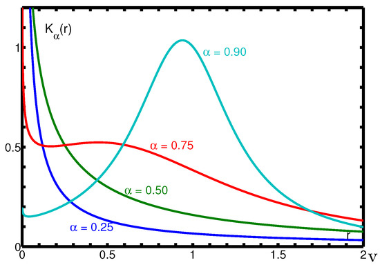
Figure 1.
The spectral function for in the frequency range .
In Figure 2, we show some plots of for some values of the parameter . It is worthwhile to note the different rates of decay of for small and large times. In fact the decay is very fast as and very slow as .
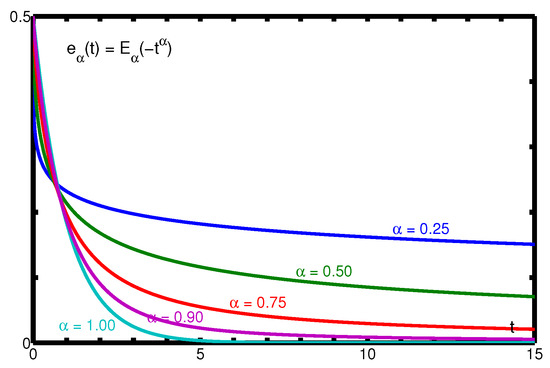
Figure 2.
The Mittag-Leffler function for in the time range .
The Mittag-Leffler function turns out the basic function in relaxation processes of physical interest occurring in viscoelastic and dielectric materials. We refer the readers for viscoelasticity, that is, to the contribution of the author including References [22,29,30] whereas for dielectric materials to the survey by Garrappa et al. [31]. For the pioneers who have pointed out the role of the Mittagf-Leffler function in mechanical and dielectric relaxation processes we refer to the recent survey by Mainardi and Consiglio [32].
4. Asymptotic Approximations to the Mittag-Lefler Function
We now report the two common asymptotic approximations of our Mittag-Leffler function. Indeed, it is common to point out that the function matches for with a stretched exponential with an infinite negative derivative, whereas as with a negative power law. The short time approximation is derived from the convergent power series representation (2). In fact,
The long time approximation is derived from the asymptotic power series representation of that turns out to be, see [6]
so that, at the first order,
As a consequence the function interpolates for intermediate time t between the stretched exponential and the negative power law. The stretched exponential models the very fast decay for small time t, whereas the asymptotic power law is due to the very slow decay for large time t. In fact, we have the two commonly stated asymptotic representations:
The stretched exponential replaces the rapidly decreasing expression from (21). Of course, for sufficiently small and for sufficiently large values of t we have the inequality
In Figure 3 and Figure 4, we compare for in logarithmic scales the function (continuous line) and its asymptotic representations, the stretched exponential valid for (dashed line) and the power law valid for (dotted line). We have chosen the time range .
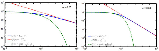
Figure 3.
Approximations (dashed line) and (dotted line) to in for (LEFT) and for (RIGHT).
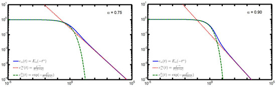
Figure 4.
Approximations (dashed line) and (dotted line) to (LEFT) and the corresponding relative errors (RIGHT) in for (LEFT) and for (RIGHT).
We note from Figure 3 and Figure 4 that, whereas the plots of remain always under the corresponding ones of , the plots of start above those of but, at a certain point, an intersection may occur so changing the sign of the relative errors. The interested reader may consul the plots of the relative errors in the 2014 paper by the author [33] from which, in particular, Figure 1, Figure 2, Figure 3 and Figure 4 have been extracted.
5. The Generalized Mittag-Leffler Function
In this survey we will devote our attention mainly to the classical Mittag-Leffler function in one parameter as introduced by Mittag-Leffler in 1903 and defined by the power series in (1). We have just learned from the instructive E-print by Van Mieghem [13] that the series (1) was discussed by Hadamard in 1893, that is 10 years earlier than Mittag-Leffler himself.
As a matter of fact a straightforward generalization of the classical Mittag-Leffler function is obtained by replacing the additive constant 1 in the argument of the Gamma function in (1) by an arbitrary complex parameter It was formerly considered in 1905 by Reference [34] and soon later by Mittag-leffler himself, almost incidentally in one of his notes. Later, in the 1950’s, such generalization was investigated by Humbert and Agarwal, with respect to the Laplace transformation, see References [35,36,37]. Usually, when dealing with Laplace transform pairs, the parameter is required to be real and positive like .
For this function we agree to use the notation
Of course . The series is still convergent for all the complex plane so the function (26) is still entire for for any
with order so the additional parameter play any role on this respect. However the Laplace transform pairs concerning the Mittag-Leffler function (26) and its derivative are known to be with and , see, for example, Refs. [14,19,22],
and
We also note the following relation concerning the first derivative of the classical Mittag-Leffler function with the two-parameter Mittag-Leffler function usually overlooked by several authors but easily proved:
We report the plot of the function herewith in Figure 5.
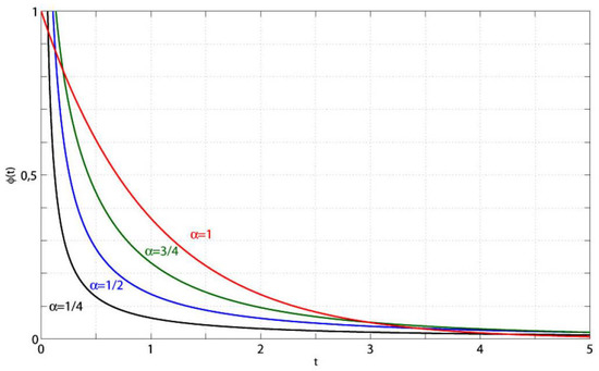
Figure 5.
Plots of with versus t; for .
We note that Mittag-Leffler functions with more than two parameters were also dealt with by several authors as pointed out in [14]. In particular, for the 3-parameter Mittag-Leffler function (known as Prabhakar function) and related operators we refer the reader to the recent survey by Giusti et al. [38] and references therein. Kiryakova has dealt in a number of papers the multi-index Mittag-Leffler functions, see for example [39].
6. The Fractional Poisson Process and the Mittag-Leffler Function
Hereafter we describe how the Mittag-Leffler function enters into the so-called fractional Poisson process. We are following the original approach by Mainardi et al. in [40] where the fractional Poisson process is referred to as the renewal process of the Mittag-Leffler type. However, an independent approach to the fractional Poisson process was given for example, by Laskin in [41].
6.1. Essentials of Renewal Theory
The concept of renewal process has been developed as a stochastic model for describing the class of counting processes for which the times between successive events are independent identically distributed () non-negative random variables, obeying a given probability law. These times are referred to as waiting times or inter-arrival times. For more details see, for example, the classical treatises by Cox [42], Feller [21].
For a renewal process having waiting times , let
That is is the time of the first renewal, is the time of the second renewal and so on. In general denotes the kth renewal.
The process is specified if we know the probability law for the waiting times. In this respect we introduce the probability density function () and the (cumulative) distribution function so defined:
When the non-negative random variable represents the lifetime of technical systems, it is common to refer to as to the failure probability and to
as to the survival probability, because and are the respective probabilities that the system does or does not fail in . A relevant quantity is the counting function defined as
that represents the effective number of events before or at instant t. In particular we have Continuing in the general theory we set , , and in general
thus represents the probability that the sum of the first k waiting times is less or equal t and its density. Then, for any fixed the normalization condition for is fulfilled because
In fact, the sum of k random variables each of which is finite with probability 1 is finite with probability 1 itself. By setting for consistency and , where for the Dirac delta generalized function in we assume the formal representation
we also note that for we have
We now find it convenient to introduce the simplified notation for the Laplace convolution between two causal well-behaved (generalized) functions and
Being the of the sum of the k random variables with we easily recognize that turns out to be the k-fold convolution of with itself,
so Equation (36) simply reads:
Because of the presence of Laplace convolutions a renewal process is suited for the Laplace transform method. Throughout this paper we will denote by the Laplace transform of a sufficiently well-behaved (generalized) function according to
and for consistently we will have Note that for our purposes we agree to take s real. We recognize that (38) reads in the Laplace domain
where, using (32),
6.2. The Classical Poisson Process as a Renewal Process
The most celebrated renewal process is the Poisson process characterized by a waiting time of exponential type,
The process has no memory. Its moments turn out to be
and the survival probability is
We know that the probability that k events occur in the interval of length t is
The probability distribution related to the sum of k exponential random variables is known to be the so-called Erlang distribution (of order k). The corresponding density (the Erlang ) is thus
so that the Erlang distribution function of order k turns out to be
In the limiting case we recover .
The results (44)–(46) can easily obtained by using the technique of the Laplace transform sketched in the previous section noting that for the Poisson process we have:
and for the Erlang distribution:
We also recall that the survival probability for the Poisson renewal process obeys the ordinary differential equation (of relaxation type)
6.3. The Renewal Process of Mittag-Leffler Type
A “fractional” generalization of the Poisson renewal process is simply obtained by generalizing the differential Equation (49) replacing there the first derivative with the integro-differential operator that is interpreted as the fractional derivative of order in Caputo’s sense, see Section 2. We write, taking for simplicity ,
We also allow the limiting case where all the results of the previous section (with ) are expected to be recovered.
For our purpose we need to recall the Mittag-Leffler function as the natural “fractional” generalization of the exponential function, that characterizes the Poisson process. We again recall that the Mittag-Leffler function of parameter is defined in the complex plane by the power series
as stated in Section 2 where the parameter was denoted by .
The solution of Equation (50) is known to be, see Section 3
so
Then, the corresponding Laplace transforms read
Hereafter, we find it convenient to summarize the most relevant features of the functions and when We begin to quote their series expansions convergent in all of suitable for and their asymptotic representations for ,
and
In contrast to the Poissonian case , in the case for large t the functions and no longer decay exponentially but algebraically. As a consequence of the power-law asymptotics the process turns out to be no longer Markovian but of long-memory type. However, we recognize that for both functions , keep the “completely monotonic” character of the Poissonian case. as can be simply derived from Section 2. We recall that complete monotonicity of our functions and means
or equivalently, their representability as real Laplace transforms of non-negative generalized functions (or measures).
For the generalizations of Equations (44)–(46), characteristic of the Poisson and Erlang distributions respectively, we must point out the Laplace transform pair
with that can be deduced from the book by Podlubny, see Equation (1.80) in Reference [19]. Then, by using the Laplace transform pairs (25) and Equations (52), (53), (58) in Equations (37) and (38), we have the generalized Poisson distribution,
and the generalized Erlang ’s (of order ),
The generalized Erlang distribution functions turn out to be
7. The Gnedenko-Kovalenko Theory of Thinning and the Mittag-Leffler Function
The thinning theory for a renewal process has been considered in detail by Gnedenko and Kovalenko [43] in the first edition of their book on Queue theory of 1968. However, the connection with the Laplace transform of the Mittag-Leffler function outlined at the end of this section in Equations (71) and (72), see also [44] and [45], is surprisingly not present in the second edition of the book by Gnedenko & Kovalenko in 1989.
We must note that other authors, like Szántai [46,47] speak of rarefaction in place of thinning.
Let us sketch here the essentials of this theory: in the interest of transparency and readability we avoid the possible decoration of the relevant power law by multiplying it with a slowly varying function.
Denoting by , the time instants of events of a renewal process, assuming , with waiting times for , (generically denoted by T), thinning (or rarefaction) means that for each positive index k a decision is made: the event happening in the instant is deleted with probability p or it is maintained with probability , . This procedure produces a thinned or rarefied renewal process with fewer events (very few events if q is near zero, the case of particular interest) in a moderate span of time.
To compensate for this loss we change the unit of time so that we still have not very few but still a moderate number of events in a moderate span of time. Such change of the unit of time is equivalent to rescaling the waiting time, multiplying it with a positive factor so that we have waiting times , and instants , in the rescaled process. Our intention is, vaguely speaking, to dispose on in relation to the rarefaction parameter q in such a way that for q near zero in some sense the “average” number of events per unit of time remains unchanged. In an asymptotic sense we will make these considerations precise.
Denoting by the probability distribution function of the (original) waiting time T, by its density ( is a generalized function generating a probability measure) so that , and analogously by and (t) the distribution and density, respectively, of the sum of k waiting times, we have recursively
Observing that after a maintained event the next one of the original process is kept with probability q but dropped in favour of the second-next with probability and, generally, events are dropped in favour of the n-th-next with probability , we get for the waiting time density of the thinned process the formula
With the modified waiting time we have
hence the density , and analogously for the density of the sum of n waiting times . The density of the waiting time of the rescaled (and thinned) process now turns out as
In the Laplace domain we have hence (using )
from which by Laplace inversion we can, in principle, construct the waiting time density of the thinned process. By rescaling we get
Being interested in stronger and stronger thinning (infinite thinning) let us now consider a scale of processes with the parameters (of rescaling) and q (of thinning), with q tending to zero under a scaling relation yet to be specified.
We have essentially two cases for the waiting time distribution: its expectation value is finite or infinite. In the first case we put
In the second case we assume a queue of power law type (dispensing with a possible decoration by a function slowly varying at infinity)
Then, by the Karamata theory (see References [21,48]) the above conditions mean in the Laplace domain
with a positive coefficient and . The case obviously corresponds to the situation with finite first moment (2.6a), whereas the case is related to a power law queue with
Now, passing to the limit of of infinite thinning under the scaling relation
between the positive parameters q and , the Laplace transform of the rescaled density in (66) of the thinned process tends for fixed s to
which corresponds to the Mittag-Leffler density
Let us remark that Gnedenko and Kovalenko obtained (71) as the Laplace transform of the limiting density but did not identify it as the Laplace transform of a Mittag-Leffler type function. Observe that in the special case we have , hence as the limiting process the Poisson process, as formerly shown in 1956 by Rényi [49].
8. The Continuous Time Random Walk (CTRW) and the Mittag-Leffler Function
The name continuous time random walk (CTRW) became popular in physics after Montroll and Weiss (just to cite the pioneers) published a celebrated series of papers on random walks for modelling diffusion processes on lattices, see, for example, Reference [50], and the book by Weiss [51] with references therein. CTRWs are rather good and general phenomenological models for diffusion, including processes of anomalous transport, that can be understood in the framework of the classical renewal theory. In fact a CTRW can be considered as a compound renewal process (a simple renewal process with reward) or a random walk subordinated to a simple renewal process. Hereafter we will mainly follow the approach by Gorenflo & Mainardi, see, for example, Reference [52].
A spatially one-dimensional CTRW is generated by a sequence of independent identically distributed () positive random waiting times each having the same probability density function and a sequence of random jumps in each having the same probability density
Let us remark that, for ease of language, we use the word density also for generalized functions in the sense of Gel’fand & Shilov [53], that can be interpreted as probability measures. Usually the probability density functions are abbreviated by . We recall that with and with .
Setting for the wandering particle makes a jump of length in instant , so that its position is for and for We require the distribution of the waiting times and that of the jumps to be independent of each other. So, we have a compound renewal process (a renewal process with reward), compare Reference [42].
By natural probabilistic arguments we arrive at the integral equation for the probability density (a density with respect to the variable x) of the particle being in point x at instant
in which denotes the Dirac generalized function, and the survival function
denotes the probability that at instant t the particle is still sitting in its starting position Clearly, Equation (73) satisfies the initial condition .
Note that the special choice
gives the pure renewal process, with position , denoting the counting function, and with jumps all of length 1 in positive direction happening at the renewal instants.
For many purposes the integral Equation (73) of CTRW can be easily treated by using the Laplace and Fourier transforms. Writing these as
then in the Laplace-Fourier domain Equation (73) reads
Introducing formally in the Laplace domain the auxiliary function
and assuming that its Laplace inverse exists, we get, following Mainardi et al. [54], in the Laplace-Fourier domain the equation
and in the space-time domain the generalized Kolmogorov-Feller equation
with , where acts as a memory function.
If the Laplace inverse of the formally introduced function does not exist, we can formally set and multiply (78) with . Then, if exists, we get in place of (79) the alternative form of the generalized Kolmogorov-Feller equation
with and acts as a memory function.
Special choices of the memory function are and , see Equations (81) and (85):
giving the exponential waiting time with
In this case we obtain in the Fourier-Laplace domain
and in the space-time domain the classical Kolmogorov-Feller equation
giving the Mittag-Leffler waiting time with
In this case we obtain in the Fourier-Laplace domain
and in the space-time domain the time fractional Kolmogorov-Feller equation
where denotes the fractional derivative of of order in the Caputo sense, see Section 3.
The time fractional Kolmogorov-Feller equation can be also expressed via the Riemann-Liouville fractional derivative , see again Section 3, that is
with . The equivalence of the two forms (88) and (89) is easily proved in the Fourier-Laplace domain by multiplying both sides of Equation (87) with the factor .
We note that the choice may be considered as a limit of the choice as . In fact, in this limit we find so so that Equations (78)–(79) reduce to Equations (83)–(84), respectively. In this case the order of the Caputo derivative reduces to 1 and that of the R-L derivative to 0, whereas the Mittag-Leffler waiting time law reduces to the exponential.
In the sequel we will formally unite the choices (i) and (ii) by defining what we call the Mittag-Leffler memory function
whose Laplace transform is
Thus we will consider the whole range by extending the Mittag-Leffler waiting time law in (86) to include the exponential law (82).
Remark 1.
Note: The probability density function for the waiting time distribution in terms of the Mittag-Leffler function was formerly given since 1995 by Hilfer [55,56,57]. In these papers the waiting time density was given with the Mittag-Leffler function in two parameters without noting the relation with the first derivative of the classical Mittag-Leffler function as stated in Equation (29). We also note that 10 years earlier Balakrishnan [58] had derived a similar expression without recognizing the Mittag-Leffler function. Like in the case of the thinning process dealt by Gnedenko-Kowalenko (see Section 7) once again the Mitag-Leffler function was unknown to the authors.
Manipulations: Rescaling and Respeeding
We now consider two types of manipulations on the CTRW by acting on its governing Equation (79) in its Laplace-Fourier representation (78).
(A): rescaling the waiting time, hence the whole time axis;
(B): respeeding the process.
(A) means change of the unit of time (measurement). We replace the random waiting time T by a waiting time , with the positive rescaling factor . Our idea is to take in order to bring into near sight the distant future so that in a moderate span of time we will have a large number of jump events. For we get the rescaled waiting time density
By decorating also the density p with an index we obtain the rescaled integral equation of the CTRW in the Laplace-Fourier domain as
where, in analogy to (77),
(B) means multiplying the quantity representing by a factor , where is the respeeding factor: means acceleration, means deceleration. In the Laplace-Fourier representation this means multiplying the RHS of Equation (78) by the factor a since the expression corresponds to .
We now chose to consider the procedures of rescaling and respeeding in their combination so that the equation in the transformed domain of the rescaled and respeeded process has the form
Clearly, the two manipulations can be discussed separately: the choice means pure rescaling, the choice means pure respeeding of the original process. In the special case we only respeed the original system; if we can counteract the compression effected by rescaling to again obtain a moderate number of events in a moderate span of time by respeeding (decelerating) with . These vague notions will become clear as soon as we consider power law waiting times.
What is the combined effect of rescaling and respeeding on the waiting time density?
In analogy to (77) and taking account of (96) we find
and so, for the deformation of the waiting time density, the essential formula
Remark 2.
The formula (99) has the same structure as the thinning formula (66) in Section 5 (just devoted to the thinning theory) by identification of a with q. In both problems we have a rescaled process defined by a time scale τ, and we send the relevant factors τ, a and q to zero under a proper relationship. However in the thinning theory the relevant independent parameter going to 0 is that of thinning (actually respeeding) whereas in the present problem it is the rescaling parameter τ.
9. Power Laws and Asymptotic Universality of the Mittag-Leffler Waiting Time Density
We have essentially two different situations for the waiting time distribution according to its first moment (the expectation value) being finite or infinite. In other words we assume for the waiting time either
or
For convenience we have dispensed in (101) with decorating by a slowly varying function at infinity with an asymptotic power law. Then, by the standard Tauberian theory (see References [21,48]) the above conditions (100)–(101) mean in the Laplace domain the (comprehensive) asymptotic form
where we have
Then, fixing s as required by the continuity theorem of probability theory for Laplace transforms, taking
and sending τ to zero, we obtain in the limit the Mittag-Leffler waiting time law. In fact, Equations (99) and (102) imply as with ,
the Laplace transform of . This formula expresses the asymptotic universality of the Mittag-Leffler waiting time law that includes the exponential law for . It can easily be generalized to the case of power laws decorated with slowly varying functions, thereby using the Tauberian theory by Karamata (see again References [21,48]).
Comment: The formula (105) says that our general power law waiting time density is gradually deformed into the Mittag-Leffler waiting time density as tends to zero.
Hence the Mittag-Leffler waiting time density is invariant against combined rescaling with τ and respeeding with .
Remark 3.
Note that Equation (107) states the self-similarity of the combined operation rescaling-respeeding for the Mittag-Leffler waiting time density. In fact, (107) implies with which means replacing the random waiting time by . As a consequences, choosing we have
Let us stress here the distinguished character of the Mittag-Leffler waiting time density . Considering its Laplace transform
we can easily prove the identity
Observing (105) we can say that is a attractor for any power law waiting time (101) under simultaneous rescaling with and respeeding with . In other words, this attraction property of the Mittag-Leffler probability distribution with respect to power law waiting times (with ) is a kind of analogy to the attraction of sums of power law jump distributions by stable distributions.
10. The Mittag-Leffler Functions W.R.T the Time Fractional Diffusion-Wave Equations and the Wright Functions
In this section we show the relations of the Mittag-Leffler function with the Wright function via Laplace and Fourier transformations, in order to provide other arguments to outline the role of the Mittag-Leffler in the Fractional Calculus. For this purpose, because of the necessity to work with two independent parameters we first recall the proper definitions of the Mittag-Leffler and the Wright function. Then we will consider the time fractional diffusion-wave equation with its fundamental solutions to the basic boundary value problem that turn out to be expressed in terms of special cases of the Wright functions, the so called F and M functions. Finally we pay attention to some noteworthy formulas for the M-Wright function, including its connections with the Mittag-Leffler function.
10.1. Definitions and Main Properties of the Wright Functions
The classical Wright function, that we denote by , is defined by the series representation convergent in the whole complex plane,
As a consequence is an entire function for all . Originally Wright assumed in connection with his investigations on the asymptotic theory of partition [59,60] and only in 1940 he considered , [61]. We note that in the Vol 3, Chapter 18 of the handbook of the Bateman Project [6], presumably for a misprint, the parameter is restricted to be non-negative, whereas the Wright functions remained practically ignored in other handbooks. In 1993 the present author, being aware only of the Bateman handbook, proved that the Wright function is entire also for in his approaches to the time fractional diffusion equation, as outlined in his papers published from 1994 to 1997, [62,63,64,65,66]. For other earlier treatments of this function we refer to the 1999 paper by Gorenflo, Luchko and Mainardi [67]).
In view of the asymptotic representation in the complex domain and of the Laplace transform the Wright functions were distinguished by the author in first kind () and second kind () as outlined e.g., in the Appendix F of his book [22].
We note that the Wright functions are entire of order hence only the first kind functions () are of exponential order whereas the second kind functions () are not of exponential order. The case is trivial since
Following the proofs in Appendix F in Reference [22] we get the following Laplace transform pairs of the Wright functions in terms of the Mittag-Leffler functions in two parameters, where r can be the time variable or the space variable )
for the first kind ()
for the second kind ()
The Wright functions of the first kind are useful to find the solutions of some (linear and non-linear) differential equations of fractional order as recently shown by Garra and Mainardi, [68].
Since the pioneering works in 1990’s by the author, noteworthy cases of Wright functions of the second kind, known as auxiliary functions F and M play fundamental roles in solving the Signalling problem and the Cauchy value problem, respectively for the time fractional diffusion-wave equation.
We first recall hereafter these auxiliary functions in terms of the Wright functions of the second kind, following their power series representations. They read
and
interrelated through
The series representations of our auxiliary functions are derived from those of in (109). We have:
and
where we have used the well-known reflection formula for the Gamma function,
10.2. The Time-Fractional Diffusion-Wave Equation and the Related Green Functions
For the reader’s convenience let us recall the main formulas for the time fractional diffusion equations and their fundamental solutions (also referred to as the Green functions) for the Cauchy and Signalling problems. For more details we refer to References [69,70].
Denoting as usual the space and time variables, and the response variable, the family of these evolution equations reads
where the time derivative of order β is intended in the Caputo sense, namely is the operator , introduced in Section 3, but for order less than 1, see Equation (10), and a is a positive constant of dimension . Thus we must distinguish the cases and . We have
It should be noted that in both cases , the time fractional derivative in the L.H.S. of Equation (117) can be removed by a suitable fractional integration, leading to alternative forms where the necessary initial conditions at explicitly appear.
For this purpose we apply to Equation (117) the fractional integral operator of order , namely
For we have:
For we have:
Then, as a matter fact, we get the integro-differential equations:
if
if
Denoting by and sufficiently well-behaved functions, the basic boundary-value problems are thus formulated as following, assuming ,
(a) Cauchy problem
(b) Signalling problem
If we must add into (122) and (123) the initial values of the first time derivative of the field variable, since in this case the corresponding fractional derivative is expressed in terms of the second order time derivative. To ensure the continuous dependence of our solution with respect to the parameter also in the transition from to we agree to assume
as it turns out from the integral forms (120)–(121).
In view of our subsequent analysis we find it convenient to set
and from now on to add the parameter to the independent space-time variables in the solutions, writing .
For the Cauchy and Signalling problems we introduce the so-called Green functions and , which represent the respective fundamental solutions, obtained when and As a consequence, the solutions of the two basic problems are obtained by a space or time convolution according to
It should be noted that in (126) because the Green function of the Cauchy problem turns out to be an even function of x. According to a usual convention, in (127) the limits of integration are extended to take into account the possibility of impulse functions centred at the extremes.
Now we recall the results obtained in 1990’s by the author that allow us to express the two Green functions in terms of the auxiliary functions and where, for ,
acts as similarity variable. Then we obtain the Green functions in the space-time domain in the form
We also recognize the following reciprocity relation for the original Green functions,
Now , are the auxiliary functions for the general case , which generalize those well known for the standard (Fourier) diffusion equation and for the standard (D’alembert) wave equation derived for and for , respectively.
10.3. Some Noteworthy Results for the Wright Function
In this survey we find worthwhile to concentrate our attention on a single auxiliary function, the M-Wright function, sometimes referred to as the Mainardi function. Indeed this function is indeed referred with this name in the 1999 book by Podlubny [19], that is one of the most cited treatises on fractional calculus. Then this name is found in several successive papers and books related to fractional diffusion and wave processes, see for example, the relevant 2015 paper by Sandev et al. [71].
Let us now recall some interesting analytic results related to the so-called Mainardi function. One reason for the major attention is due to its straightforward generalization of the Gaussian probability density obtained for , that is the fundamental solution of the Cauchy problem for the standard diffusion equation. Furthermore it allows an impressive visualization of the evolution with the order of the Green function of the Cauchy problem of the fractional diffusion wave Equation (129) as shown in the next figures with and taking .
The readers are invited to look at the YouTube video by my former student Armando Consiglio whose title is “Simulation of the Wright function”, in which the author has shown the evolution of this function as the parameter changes between 0 and 0.85 in the interval () of centered in represented herewith in Figure 6 and Figure 7 at fixed time .
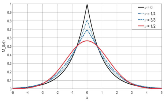
Figure 6.
Plot of the symmetric Wright function for . Note that the -Wright function becomes a Gaussian density for .
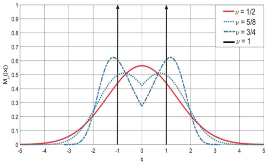
Figure 7.
Plot of the symmetric Wright type function for . Note that the MWright function becomes a a sum of two delta functions centered in for .
The readers interested to have more details on the classical Wright functions should consult the recent survey by Luchko [72] and references therein.
In view of time-fractional diffusion processes related to time-fractional diffusion equations it is worthwhile to introduce the function in two variables
which defines a spatial probability density in x evolving in time t with self-similarity exponent . Of course for we have to consider the symmetric version of the M-Wright function. obtained from (132) multiplying by and replacing x by .
Hereafter we provide a list of the main properties of this function, which can be derived from the Laplace and Fourier transforms for the corresponding Wright M-function in one variable presented in papers by Mainardi and recalled in the Appendix F of Reference [22].
For the Laplace transform of with respect to and we get respectively:
For the Fourier transforms with respect to the spatial variable x we have for with ,
so that for the symmetric function we get
Restricting our attention at the known analytic expressions of the functions versus x at fixed time we recall the following results for some special rational values of the parameter :
(see Reference [22])
(see Reference [22])
(see Reference [73])
In the above equations Ai and denote the Airy function and its first derivative.
Funding
This research received no external funding.
Acknowledgments
The work of the author has been carried out in the framework of the activities of the National Group of Mathematical Physics (GNFM, INdAM). The author would like to thank the anonymous reviewers for their helpful and constructive comments and Bruce West for the invitation.
Conflicts of Interest
The author declares no conflict of interest.
Appendix A. My Acquaintance with the Mittag-Leffler Function Since the Late 1960’s
I was formerly acquainted with the Mittag-Leffler function from the pioneering 1947 paper by Gross on creep and relaxation in linear viscoelasticity. It was during my PhD studies at the University of Bologna under the supervision of Prof Caputo in the year 1969. Indeed I was asked to apply in the framework of anelastic materials the derivative of non-integer order introduced by Prof Caputo in [74,75]. More recently this fractional derivative was named after him thanks the suggestions of Gotrenflo and Mainardi [18] and Podlubny [19]. I understood that the Mittag-Leffler function proposed by Gross both in creep and relaxation processes could be used in the corresponding processes in the fractional Zener model. Because Gross had computed and plotted only the spectra, see Figure 1 in this article, I was interested to plot the Mittag-Leffler function on which I was addressed in the Third volume of the Handbook of the Bateman Project published in 1955 [6]. Carrying out the plot of the Mittag-Leffler function using a Fortran program was not easy for me using its power series representation, so I limited the time interval to with ordinate in logarithmic scale. As far as I know this was the former plot of this function, see References [9,10] where the results of my PhD thesis were published in 1971 jointly with my supervisor. Later I was acquainted with the viscoelastic model by Rabotnov in 1948 [76] and with the Russian school of Meskov and Rossikhin who used the so-called Rabotnov function, indeed related to the Mittag-Leffler function, and consequently with results similar to some extent to those in References [9,10]. However, our work was totally independent from the Russian school (incidentally published in Russian), as outlined in the Notes to the chapter 3 of my 2010 book, see pp. 74–76 in [22]. More later, in the 1980 I was acquainted with the results by Bagley-Torvik and by Koeller that confirmed the relevant role of the Mittag-Leffler functions in linear viscoelastic models governed by constitutive laws of fractional order. Once again their results crossed with those in References [9,10]. However, I have to confess that, when in conferences of those years I dealt with fractional derivatives in rheology, the audience remained indifferent if not hostile and laughable so I left this topic preferring to transfer my research interests to wave phenomena, in particular on the effects of dissipation on linear dispersive waves.
Incidentally, in 1980’s, I was also aware of the nice treatise by Harold T. Davis on the Theory of Linear operators published in 1936 [2], where the author gave information about the fractional calculus and the Mittag-Leffler function. It was my honor to publish a recent survey on the contributions by Davis and Gross (already recalled in Introduction), whom I consider the pioneers of fractional relaxation processes in viscoelastic and dielectric materials [32]. In the firsts years of 1990s under the push of fractals, the relevance of fractional derivatives (used not always in a correct way) was outlined in several papers. For this I was induced to come back to fractional calculus. It was just this occasion for me to devote my research interests to the application of fractional calculus in relaxation, oscillation phenomena governed by fractional ODEs and diffusion, wave phenomena governed by fractional PDEs. Once again I understood the relevance of the Mittag-Leffler functions but also that of the Wright functions, both of them classified as miscellaneous functions in the handbook of Bateman project. I must note that, as far as I known, the Bateman handbook was the only one published in English to deal with these special function, and therefore accessible to me.
The year 1994 was the golden year for me as far as my acquaintance with fractional calculus and related special functions is concerned. Indeed I took profit by the acquaintance in three different conferences with the late Prof Gorenflo and Prof. Nigmatullin (in Bordeaux, France), with Prof. Podlubny and Prof. Caputo (in Atlanta, USA), and with Prof Virginia Kiryakova and the late Prof. Stankovic (in Sofia, Bulgaria), among other authorities of the fractional calculus. But it was with Prof Gorenflo that I started a collaboration for more than 20 years (1995–2015) motivated by our common interest towards the potential of the Mittag-Leffler functions in the applications of the fractional calculus.
Then, since 1997, I was interested in the emerging science of Econophysics thanks mainly to my younger colleague Enrico Scalas. With Gorenflo, Scalas and his student Raberto we published some papers on the advent of fractional Calculus in Econophysics, see e.g., [54] and my historical survey in Mathematics [77]. In 2007, on the occasion of the 80-birthday of Prof. Caputo, I published with Gorenflo a survey in Fractional Calculus and Applied Analysis [11] where I took the liberty to propose for the Mittag-Leffler function the (successful) title of the Queen Function of the Fractional Calculus. Some years earlier, Gorenflo had contacted the American Mathematical Society to give a specific number to the Mittag-Leffler function, that is 33E12, in the MSC classification.
Gorenflo and I promoted the Mittag-Lffler functions in several Conferences and Workshops in all the world. In particular, I would like to recall my lectures in India (under invitation of Prof Mathai, director of the Center of Mathematical Sciences, in Brazil (under invitation of Prof Edmundo Capelas de Oliveira, Campinas University) and in US (under invitation of Prof. Karniadakis, Brown University, see Reference [78]).
I like to outline my gratitude to Professor Michele Caputo (1927) and Rudolf Gorenflo (1930–2017) for having provided me with useful advice in earlier and later times, respectively. It is my pleasure to enclose a photo showing the author between them, taken in Bologna, April 2002.

Figure A1.
F. Mainardi between R. Gorenflo (left) and M. Caputo (right).
Unfortunately, I lost Gorenflo’s guidance and collaboration in 2015 when he suffered strong health troubles that led him to his death on 20 October 2017 at 87 years. He was Emeritus Professor of Mathematics at the Free University of Berlin since his retirement in 1998.
Nowadays I am quite interested to promote the special functions of the Mittag-Leffler and Wright type with the second edition of the treatise by Gorenflo et al. [14] and my surveys [79,80], including the present review.
References
- Hille, E.; Tamarkin, J.D. On the theory of linear integral equations. Ann. Math. 1930, 31, 479–528. [Google Scholar] [CrossRef]
- Davis, H.T. The Theory of Linear Operators; The Principia Press: Bloomington, Indiana, 1936. [Google Scholar]
- Sansone, G.; Gerretsen, J. Lectures on the Theory of Functions of a Complex Variable; Holomorphic Functions: Nordhoff, Groningen, 1960; Volume I. [Google Scholar]
- Dzherbashyan, M.M. Integral Transforms and Representations of Functions in the Complex Plane; Nauka: Moscow, Russia, 1966. (In Russian) [Google Scholar]
- Samko, S.G.; Kilbas, A.A.; Marichev, O.I. Fractional Integrals and Derivatives, Theory and Applications; Gordon and Breach: Amsterdam, The Netherlands, 1993. [Google Scholar]
- Erdélyi, A.; Magnus, W.; Oberhettinger, F.; Tricomi, F. Higher Transcendental Functions; McGraw-Hill: New York, NY, USA, 1955; Volume 3. [Google Scholar]
- Cole, K.S.; Cole, R.H. Dispersion and absorption in dielectrics, II. Direct current characteristics. J. Chem. Phys. 1942, 10, 98–105. [Google Scholar] [CrossRef]
- Gross, B. On creep and relaxation. J. Appl. Phys. 1947, 18, 212–221. [Google Scholar] [CrossRef]
- Caputo, M.; Mainardi, F. A new dissipation model based on memory mechanism. Pure Appl. Geophys. (PAGEOPH) 1971, 91, 134–147, Reprinted in Fract. Calc. Appl. Anal. 2007, 10, 309–324. [Google Scholar] [CrossRef]
- Caputo, M.; Mainardi, F. Linear models of dissipation in anelastic solids. Riv. Nuovo Cimento 1971, 1, 161–198. [Google Scholar] [CrossRef]
- Mainardi, F.; Gorenflo, R. Time-Fractional Derivatives in Relaxation Processes: A Tutorial Survey. Fract. Calc. Appl. Anal. 2007, 10, 269–308. [Google Scholar]
- Haubold, H.J.; Mathai, A.M.; Saxena, R.K. Mittag-Leffler functions and their applications. J. Appl. Math. 2011, 2011, 298628. [Google Scholar] [CrossRef]
- Van Mieghem, P. The Mittag-Leffler funcytion. arXiv 2005, arXiv:2005.13330. [Google Scholar]
- Gorenflo, R.; Kilbas, A.A.; Mainardi, F.; Rogosin, S. Mittag-Leffler Functions. Related Topics and Applications, 2nd ed.; Springer: Berlin, Germany, 2020. [Google Scholar]
- Mainardi, F.; Pironi, P. The fractional Langevin equation: Brownian motion revisited. Extr. Math. 1996, 11, 140–154. [Google Scholar]
- Mainardi, F.; Mura, A.; Tampieri, F. Brownian motion and anomalous diffusion revisited via a fractional Langevin equation. Mod. Probl. Stat. Phys. 2009, 8, 3–23. [Google Scholar]
- Sandev, T.; Tomovoski, Ž. Fractional Equations and Models. Theory and Applications; Springer: Cham, Switzerland, 2019. [Google Scholar]
- Gorenflo, R.; Mainardi, F. Fractional Calculus: Integral and Differential Equations of Fractional Order. In Fractals and Fractional Calculus in Continuum Mechanics; Carpinteri, A., Mainardi, F., Eds.; Springer: New York, NY, USA, 1997; pp. 223–276. [Google Scholar]
- Podlubny, I. Fractional Differential Equations; Academic Press: San Diego, CA, USA, 1999. [Google Scholar]
- Pollard, H. The completely monotonic character of the Mittag-Leffler function Eα(−x). Bull. Am. Math. Soc. 1948, 54, 1115–1116. [Google Scholar] [CrossRef]
- Feller, W. An Introduction to Probability Theory and Its Applications, 2nd ed.; Wiley: New York, NY, USA, 1971; Volume II, First edition (1966). [Google Scholar]
- Mainardi, F. Fractional Calculus and Waves in Linear Viscoelasticity; Imperial College Press: London, UK, 2010; Second edition in preparation. [Google Scholar]
- Miller, K.S.; Samko, S.G. Completely monotonic functions. Integr. Transf. Spec. Funct. 2001, 12, 389–402. [Google Scholar] [CrossRef]
- Schilling, R.L.; Song, R.; Vondracek, Z. Bernstein Functions. Theory and Applications, 2nd ed.; De Gruyter: Berlin, Germny, 2012. [Google Scholar]
- Titchmarsh, E.C. Introduction to the Theory of Fourier Integrals; Oxford University Press: Oxford, UK, 1937. [Google Scholar]
- Gross, B.; Levi, B. Sobra el calculo de la transformacio inverse de Laplace. Math. Notae 1946, 6, 213–224. [Google Scholar]
- Gross, B. Note on the inversion of the Laplace transform. Philos. Mag. 1950, 41, 543–544. [Google Scholar] [CrossRef]
- Apelblat, A. Integral Transforms and Volterra Functions; Nova Publisher: New York, NY, USA, 2011. [Google Scholar]
- Mainardi, F. Fractional viscoelasticity. In Handbook of Fractional Calculus with Applications; Tarasov, V., Ed.; De Gruyter GmbH: Berlin, Germany, 2019; Volume 5, pp. 153–182. [Google Scholar]
- Mainardi, F.; Spada, G. Creep, relaxation and viscosity properties for basic fractional models in rheology. Eur. Phys. J. 2011, 193, 133–160. [Google Scholar] [CrossRef]
- Garrappa, R.; Mainardi, F.; Maione, G. Models of dielectric relaxation based on completely monotone functions. Fract. Calc. Appl. Anal. 2016, 19, 1105–1160. [Google Scholar] [CrossRef]
- Mainardi, F.; Consiglio, A. The pioneers of the Mittag-Leffler functions in dielectrical and mechanical relaxation processes. WSEAS Trans. Math. 2020, 19, 289–300. [Google Scholar] [CrossRef]
- Mainardi, F. On some properties of the Mittag-Leffler function Eα(−tα), completely monotone for t > 0 with 0 < α < 1. Discret. Contin. Dyn. Syst. Ser. B 2014, 19, 2267–2278. [Google Scholar] [CrossRef]
- Wiman, A. Über den Fundamentalsatz der Theorie der Funkntionen Eα(x). Acta Math. 1905, 29, 191–201. [Google Scholar] [CrossRef]
- Humbert, P. Quelques résultats relatifs à la fonction de Mittag-Leffler. C. R. Acad. Sci. Paris 1953, 236, 1467–1468. [Google Scholar]
- Agarwal, R.P. A propos d’une note de M. Pierre Humbert. C. R. Acad. Sci. Paris 1953, 236, 2031–2032. [Google Scholar]
- Humbert, P.; Agarwal, R.P. Sur la fonction de Mittag-Leffler et quelques-unes de ses généralisations. Bull. Sci. Math. 1953, 77, 180–185. [Google Scholar]
- Giusti, A.; Colombaro, I.; Garra, R.; Garrappa, R.; Polito, F.; Popolizio, M.; Mainardi, F. A Guide to Prabhakar functions and operators. Fract. Calc. Appl. Anal. 2020, 23, 9–54. [Google Scholar] [CrossRef]
- Kiryakova, V. The multi-index Mittag-Leffler functions as an important class of special functions of fractional calculus. Comp. Math. Appl. 2010, 59, 1885–1895. [Google Scholar] [CrossRef]
- Mainardi, F.; Gorenflo, R.; Scalas, E. A fractional generalization of the Poisson processes. Vietnam J. Math. 2004, 32, 53–64. [Google Scholar]
- Laskin, N. Fractional Poisson processes. Comm. Nonlinear Sci. Num. Sim. 2003, 8, 201–213. [Google Scholar] [CrossRef]
- Cox, D.R. Renewal Theory, 2nd ed.; Methuen: London, UK, 1967. [Google Scholar]
- Gnrdenko, B.V.; Kowalenko, I.N. Introduction to Queueing Theory; Israel Program for Scientific Translations: Jerusalem, Israel, 1968. [Google Scholar]
- Gorenflo, R.; Mainardi, F. Continuous time random walk, Mittag-Leffler waiting time and fractional diffusion: Mathematical aspects, Chapter 4. In Anomalous Transport: Foundations and Applications; Klages, R., Radons, G., Sokolov, I.M., Eds.; Wiley-VCH: Weinheim, Germany, 2008; pp. 93–127. [Google Scholar]
- Gorenflo, R.; Mainardi, F. The Mittag-Leffler function in the thinning theory for renewal processes. Theory Probab. Math. Stat. 2018, 98, 100–108. [Google Scholar] [CrossRef]
- Szàntai, T. Limiting distribution for the sums of random number of random variables concerning the rarefaction of recurrent events. Stud. Sci. Math. Hung. 1971, 6, 443–452. [Google Scholar]
- Szàntai, T. On an invariance problem related to different rarefactions of recurrent events. Stud. Sci. Math. Hung. 1971, 6, 453–456. [Google Scholar]
- Widder, D.V. The Laplace Transform; Princeton University Press: Princeton, NJ, USA, 1946. [Google Scholar]
- Renyi, A. A characteristic of the Poisson stream. Proc. Math. Inst. Hung. Acad. Sci. 1956, 1, 563–570. (In Hungarian) [Google Scholar]
- Montroll, E.W.; Weiss, G.H. Random walks on lattices, II. J. Math. Phys. 1965, 6, 167–181. [Google Scholar] [CrossRef]
- Weiss, G.H. Aspects and Applications of Random Walks; North-Holland: Amsterdam, The Netherlands, 1994. [Google Scholar]
- Gorenflo, R.; Mainardi, F. Parametric Subordination in Fractional Diffusion Processes. In Fractional Dynamics, Recent Advances; Klafter, J., Lim, S.C., Metzler, R., Eds.; World Scientific: Singapore, 2012; Chapter 10; pp. 227–261. [Google Scholar]
- Gelf, I.M.; Shilov, G.E. Generalized Functions; Academic Press: New York, NY, USA, 1964; Volume 1. [Google Scholar]
- Mainardi, F.; Raberto, M.; Gorenflo, R.; Scalas, E. Fractional calculus and continuous-time finance II: The waiting time distribution. Phys. A 2000, 287, 468–481. [Google Scholar] [CrossRef]
- Hilfer, R. Exact solutions for a class of fractal time random walks. Fractals 1995, 3, 211–216. [Google Scholar] [CrossRef]
- Hilfer, R. On fractional diffusion and continuous time random walks. Phys. A 2003, 329, 35–39. [Google Scholar] [CrossRef]
- Hilfer, R.; Anton, L. Fractional master equations and fractal time random walks. Phys. Rev. E 1995, 51, R848–R851. [Google Scholar] [CrossRef]
- Balakrishnan, V. Anomalous diffusion in one dimension. Phys. A 1985, 132, 569–580. [Google Scholar] [CrossRef]
- Wright, E.M. On the coefficients of power series having exponential singularities. J. Lond. Math. Soc. 1933, 8, 71–79. [Google Scholar] [CrossRef]
- Wright, E.M. The asymptotic expansion of the generalized Bessel function. Proc. Lond. Math. Soc. (Ser. II) 1935, 38, 257–270. [Google Scholar] [CrossRef]
- Wright, E.M. The generalized Bessel function of order greater than one. Quart. J. Math. Oxf. Ser. 1940, 11, 36–48. [Google Scholar] [CrossRef]
- Mainardi, F. On the initial value problem for the fractional diffusion-wave equation. In Waves and Stability in Continuous Media; Rionero, S., Ruggeri, T., Eds.; World Scientific: Singapore, 1994; pp. 246–251. [Google Scholar]
- Mainardi, F. The Time Fractional Diffusion-Wave-Equation. Radiophys. Quantum Electron. 1995, 38, 20–36. [Google Scholar] [CrossRef]
- Mainardi, F. The Fundamental Solutions for the Fractional Diffusion-Wave Equation. Appl. Math. Lett. 1996, 9, 23–28. [Google Scholar] [CrossRef]
- Mainardi, F. Fractional Relaxation-Oscillation and Fractional Diffusion-Wave Phenomena. Chaos Solitons Fractals 1996, 7, 1461–1477. [Google Scholar] [CrossRef]
- Mainardi, F. Fractional Calculus: Some Basic Problems in Continuum and Statistical Mechanics. In Fractals and Fractional Calculus in Continuum Mechanics; Carpinteri, A., Mainardi, F., Eds.; Springer: New York, NY, USA, 1997; pp. 291–348. [Google Scholar]
- Gorenflo, R.; Luchko, Y.; Mainardi, F. Analytical Properties and Applications of the Wright Function. Fract. Calc. Appl. Anal. 1999, 2, 383–414. [Google Scholar]
- Garra, R.; Mainardi, F. Some aspects of Wright functions in fractional differential equations. arXiv 2020, arXiv:2007.13340. [Google Scholar]
- Mainardi, F.; Luchko, Y.; Pagnini, G. The Fundamental Solution of the Space-Time Fractional Diffusion Equation. Fract. Calc. Appl. Anal. 2001, 4, 153–192. [Google Scholar]
- Luchko, Y.; Mainardi, F. Fractional diffusion-wave hhenomena. In Handbook of Fractional Calculus with Applications; Tarasov, V., Ed.; De Gruyter GmbH: Berlin, Germany, 2019; Volume 5, pp. 71–98. [Google Scholar]
- Sandev, T.; Chechkin, A.V.; Korabel, N.; Kantz, H.; Sokolov, I.M.; Metzler, R. Distributed-order diffusion equations and multifractality: Models and solutions. Phys. Rev. E 2015, 92, 042117. [Google Scholar] [CrossRef]
- Luchko, Y. The Wright function and its applications. In Handbook of Fractional Calculus with Applications; Kochubei, A., Luchko, Y., Eds.; De Gruyter GmbH: Berlin, Germany, 2019; Volume 1, pp. 241–268. [Google Scholar]
- Hanyga, A. Multidimensional solutions of time-fractional diffusion-wave equations. Proc. R. Soc. Lond. Ser. A 2002, 458, 933–957. [Google Scholar] [CrossRef]
- Caputo, M. Linear models of dissipation whose Q is almost frequency independent, Part II. Geophys. J. R. Astr. Soc. 1967, 13, 529–539, Reprinted in Fract. Calc. Appl. Anal. 2008, 11, 4–14. [Google Scholar] [CrossRef]
- Caputo, M. Elasticità e Dissipazione; Zanichelli: Bologna, Italy, 1969. (In Italian) [Google Scholar]
- Rabotnov, Y.N. Equilibrium of an elastic medium with after effect. Prikl. Matem. i Mekh. (PMM) 1948, 12, 81–91. (In Russian) [Google Scholar] [CrossRef]
- Mainardi, F. On the Advent of Fractional Calculus in Econophysics via Continuous-Time Random Walk. Mathematics 2020, 8, 641. [Google Scholar] [CrossRef]
- Mainardi, F. A Course on Fractional Calculus. Available online: www.brown.edu/academics/applied-mathematics/teaching-schedule/fractional-calculus-lecture-notes (accessed on 29 November 2020).
- Mainardi, F. A tutorial on the basic special functions of Fractional Calculus. WSEAS Trans. Math. 2020, 19, 74–98. [Google Scholar] [CrossRef]
- Mainardi, F.; Consiglio, A. The Wright functions of the second kind in Mathematical Physics. Mathematics 2020, 8, 884. [Google Scholar] [CrossRef]
Publisher’s Note: MDPI stays neutral with regard to jurisdictional claims in published maps and institutional affiliations. |
© 2020 by the author. Licensee MDPI, Basel, Switzerland. This article is an open access article distributed under the terms and conditions of the Creative Commons Attribution (CC BY) license (http://creativecommons.org/licenses/by/4.0/).