Optimization of Selective Assembly for Shafts and Holes Based on Relative Entropy and Dynamic Programming

Abstract
1. Introduction
2. Related Works
3. Method
3.1. Selective Assembly Optimization Model for Shaft and Hole
3.2. Clearance Uniformity Evaluation of Shaft and Hole Based on Relative Entropy
3.3. Optimization Algorithm Based on Dynamic Programming
4. Case Study
5. Results and Discussion
6. Conclusions and Future Work
Author Contributions
Funding
Conflicts of Interest
References
- Wang, X. Mechanical Manufacturing Technology; China Machine Press: Beijing, China, 2013. [Google Scholar]
- Zhang, Q.; Zhang, Z.; Jin, X.; Zeng, W.; Lou, S.; Jiang, X.; Zhang, Z. Entropy-based method for evaluating spatial distribution of form errors for precision assembly. Precis. Eng. 2019, 60, 374–382. [Google Scholar] [CrossRef]
- STANDARD A. Dimensioning and Tolerancing; ASME Y14.5M-2009; American Society of Mechanical Engineers: New York, NY, USA, 2009. [Google Scholar]
- Chen, X.; Jin, X.; Shang, K.; Zhang, Z. Entropy-Based Method to Evaluate Contact-Pressure Distribution for Assembly-Accuracy Stability Prediction. Entropy 2019, 21, 322. [Google Scholar] [CrossRef]
- Kannan, S.M.; Jeevanantham, A.K.; Jayabalan, V. Modelling and analysis of selective assembly using Taguchi’s loss function. Int. J. Prod. Res. 2008, 46, 4309–4330. [Google Scholar] [CrossRef]
- Tu, Z. Research on Technologies of Structural Layout and Matching Optimization for Customized Product; Zhejiang University: Hangzhou, China, 2013. [Google Scholar]
- Matsuura, S. Optimal Partitioning of Probability Distributions under General Convex Loss Functions in Selective Assembly. Commun. Stats. 2011, 40, 1545–1560. [Google Scholar] [CrossRef]
- Lin, J.; Yang, L.; Liu, M.; Wu, J.; Zhang, F. Study on Optimization Model of Matching Parts Assembly Based on the Process Capability Index. Trans. Chin. Soc. Agric. Mach. 2007, 4. [Google Scholar] [CrossRef]
- Biao, S. Research on Selective Assembly Method Optimization for Construction Machinery Remanufacturing Based on Ant Colony Algorithm. J. Mech. Eng. 2017, 53, 60. [Google Scholar]
- Sun, Z.; Xia, P.; Yao, Y. Application study of selective assembly optimization on complex assembly. Mach. Des. Manuf. 2008, 1, 147–149. [Google Scholar]
- Asha, A.; Babu, J.R. Comparison of clearance variation using selective assembly and metaheuristic approach. Int. J. Latest Trends Eng. Technol. 2018, 8, 148–155. [Google Scholar]
- Jiang, X.; Wang, W.; Zhang, H.; Zhang, K.; Li, L. Optimal Selective Assembly Method for Remanufacturing Product Considering Quality, Cost and Resource Utilization. J. Mech. Eng. 2019. [Google Scholar] [CrossRef]
- Asha, A.; Kannan, S.; Jayabalan, V. Optimization of clearance variation in selective assembly for components with multiple characteristics. Int. J. Adv. Manuf. Technol. 2008, 38, 1026–1044. [Google Scholar] [CrossRef]
- Kannan, S.M.; Sivasubramanian, R.; Jayabalan, V. Particle swarm optimization for minimizing assembly variation in selective assembly. Int. J. Adv. Manuf. Technol. 2009, 42, 793–803. [Google Scholar] [CrossRef]
- Dong, Z.; Zhi-Yong, C.; Rong, M.O. Application particle swarm optimization in computer aided selective assembly. Comput. Eng. Appl. 2009, 45, 208–211. [Google Scholar]
- Liu, X. Algorithm Research on Computer Aided Selective Assembly; Jilin University: Changchun, China, 2006. [Google Scholar]
- Re, S.; Liu, J.; He, Y.; Jiang, K.; Guo, C. Selective assembly method for mechanical products with multiple quality requirements. Comput. Integr. Manuf. Syst. 2014, 20, 2117–2126. [Google Scholar]
- Zhang, Z. Manufacturing complexity and its measurement based on entropy models. Int. J. Adv. Manuf. Technol. 2012, 62, 867–873. [Google Scholar] [CrossRef]
- Lv, S.; Qiao, L. A cross-entropy-based approach for the optimization of flexible process planning. Int. J. Adv. Manuf. Technol. 2013, 68, 2099–2110. [Google Scholar] [CrossRef]
- Wang, M.; Xi, L.; Du, S. 3D surface form error evaluation using high definition metrology. Precis. Eng. 2014, 38, 230–236. [Google Scholar] [CrossRef]
- Mohammad-Djafari, A. Entropy, Information Theory, Information Geometry and Bayesian Inference in Data, Signal and Image Processing and Inverse Problems. Entropy 2015, 17, 3989. [Google Scholar] [CrossRef]
- Jin, X.; Zuo, F.; Zhang, T.; Zhang, Z.; Chen, J.; Ye, X. An entropy-based method to evaluate plane form error for precision assembly. Proc. Inst. Mech. Eng. Part B J. Eng. Manuf. 2013, 227, 726–734. [Google Scholar] [CrossRef]
- Fang, Y.; Jin, X.; Huang, C.; Zhang, Z. Entropy-Based Method for Evaluating Contact Strain-Energy Distribution for Assembly Accuracy Prediction. Entropy 2017, 19, 49. [Google Scholar] [CrossRef]
- Bellman, R.E.; Dreyfus, S.E. Dynamic Programming; Dover Publications, Incorporated: New York, NY, USA, 2003. [Google Scholar]
- Li, Z.; Ma, L.; Zhang, H. Cellular bat algorithm for 0–1 programming problem. Appl. Res. Comput. 2013, 30, 2903–2906. [Google Scholar]


| Material | Elastic Modulus (Gpa) | Poisson’s Ratio | Coefficient of Linear Expansion(/K−1) | Density (t/mm3) |
|---|---|---|---|---|
| Beryllium alloy | 303 | 0.025 | 11 × 10−6 | 1.85 × 10⁻⁹ |
| Shafts | Holes | |||||||
|---|---|---|---|---|---|---|---|---|
| No. | Minimum Radii | Maximum Radii | No. | Minimum Radii | Maximum radii | No. | Minimum Radii | Maximum Radii |
| 1 | 2.994 | 2.997 | 1 | 3.0005 | 3.0031 | 11 | 2.9994 | 3.0022 |
| 2 | 2.9943 | 2.9966 | 2 | 2.9962 | 3.0047 | 12 | 2.9975 | 3.0031 |
| 3 | 2.9947 | 2.9961 | 3 | 3.0002 | 3.0082 | 13 | 3.0009 | 3.0029 |
| 4 | 2.9941 | 2.9964 | 4 | 3.0001 | 3.0034 | 14 | 3.0009 | 3.003 |
| 5 | 2.9922 | 2.9954 | 5 | 2.9991 | 3.0027 | 15 | 3.0009 | 3.0022 |
| 6 | 2.9936 | 2.9975 | 6 | 2.9982 | 3.0029 | 16 | 3.0004 | 3.0022 |
| 7 | 2.9939 | 2.9953 | 7 | 2.999 | 3.0036 | 17 | 2.9991 | 3.0014 |
| 8 | 2.9932 | 2.9971 | 8 | 2.9989 | 3.004 | 18 | 3.0008 | 3.0017 |
| 9 | 3.0006 | 3.0036 | 19 | 2.9973 | 3.0008 | |||
| 10 | 3.0015 | 3.0032 | 20 | 2.9998 | 3.0021 | |||
| Shafts | Holes | ||||
|---|---|---|---|---|---|
| No. | Cylindricity | No. | Cylindricity | No. | Cylindricity |
| 1 | 0.0035 | 1 | 0.0026 | 11 | 0.0069 |
| 2 | 0.0027 | 2 | 0.0071 | 12 | 0.0068 |
| 3 | 0.002 | 3 | 0.008 | 13 | 0.0036 |
| 4 | 0.0044 | 4 | 0.0033 | 14 | 0.005 |
| 5 | 0.0037 | 5 | 0.0036 | 15 | 0.0035 |
| 6 | 0.0027 | 6 | 0.0047 | 16 | 0.0035 |
| 7 | 0.0018 | 7 | 0.0046 | 17 | 0.0036 |
| 8 | 0.0044 | 8 | 0.0051 | 18 | 0.0019 |
| 9 | 0.003 | 19 | 0.0027 | ||
| 10 | 0.0047 | 20 | 0.0034 | ||
| Holes\Shafts | 1 | 2 | 3 | 4 | 5 | 6 | 7 | 8 |
|---|---|---|---|---|---|---|---|---|
| 1 | 0.2439 | 0.2255 | 0.1040 | 0.2245 | 0.1933 | 0.2368 | 0.0959 | 0.1919 |
| 2 | - | - | - | - | - | - | - | - |
| 3 | 0.4540 | 0.1721 | 0.1972 | 0.0912 | 0.1644 | 0.0318 | 0.1973 | 0.3017 |
| 4 | 0.4155 | 0.1445 | 0.2049 | 0.1722 | 0.2488 | 0.2054 | 0.2165 | 0.1576 |
| 5 | 0.2111 | 0.4210 | 0.2936 | 0.4207 | 0.3122 | 0.3057 | 0.3219 | 0.4468 |
| 6 | 0.2980 | 0.2615 | 0.1444 | 0.2580 | 0.2295 | 0.2583 | 0.1359 | 0.2382 |
| 7 | 0.1954 | 0.2641 | 0.1430 | 0.2727 | 0.2474 | 0.2643 | 0.1478 | 0.2312 |
| 8 | 0.3576 | 0.3352 | 0.1978 | 0.2938 | 0.1701 | 0.1904 | 0.2335 | 0.3884 |
| 9 | 0.3436 | 0.1877 | 0.2614 | 0.2629 | 0.3152 | 0.3056 | 0.2882 | 0.1497 |
| 10 | 0.2211 | 0.3112 | 0.2150 | 0.3507 | 0.3239 | 0.3500 | 0.2330 | 0.2552 |
| 11 | 0.4308 | 0.1642 | 0.2013 | 0.1791 | 0.2385 | 0.2023 | 0.2059 | 0.1807 |
| 12 | 0.5256 | 0.1674 | 0.2172 | 0.1663 | 0.2569 | 0.2026 | 0.2101 | 0.1974 |
| 13 | 0.2844 | 0.2621 | 0.1260 | 0.2533 | 0.1993 | 0.2478 | 0.1167 | 0.2357 |
| 14 | 0.4141 | 0.1807 | 0.2369 | 0.2038 | 0.2706 | 0.2162 | 0.2519 | 0.2067 |
| 15 | 0.2162 | 0.2773 | 0.1767 | 0.3022 | 0.2779 | 0.2997 | 0.1904 | 0.2370 |
| 16 | 0.1849 | 0.2554 | 0.1441 | 0.2202 | 0.0912 | 0.0948 | 0.1969 | 0.3254 |
| 17 | 0.4377 | 0.1970 | 0.2483 | 0.2162 | 0.2874 | 0.2273 | 0.2599 | 0.2226 |
| 18 | 0.3847 | 0.2124 | 0.2733 | 0.2752 | 0.3244 | 0.3062 | 0.2940 | 0.1877 |
| 19 | 0.2219 | 0.2063 | 0.0782 | 0.1989 | 0.1721 | - | 0.0641 | 0.1682 |
| 20 | 0.2344 | 0.2825 | 0.1683 | 0.3069 | 0.2845 | 0.3191 | 0.1716 | 0.2294 |
| Index of Shafts | Index of Holes | Relative Entropy |
|---|---|---|
| 1 | 7 | 0.1954 |
| 2 | 4 | 0.1445 |
| 3 | 1 | 0.1040 |
| 4 | 12 | 0.1663 |
| 5 | 16 | 0.0912 |
| 6 | 3 | 0.0318 |
| 7 | 19 | 0.0641 |
| 8 | 9 | 0.1497 |
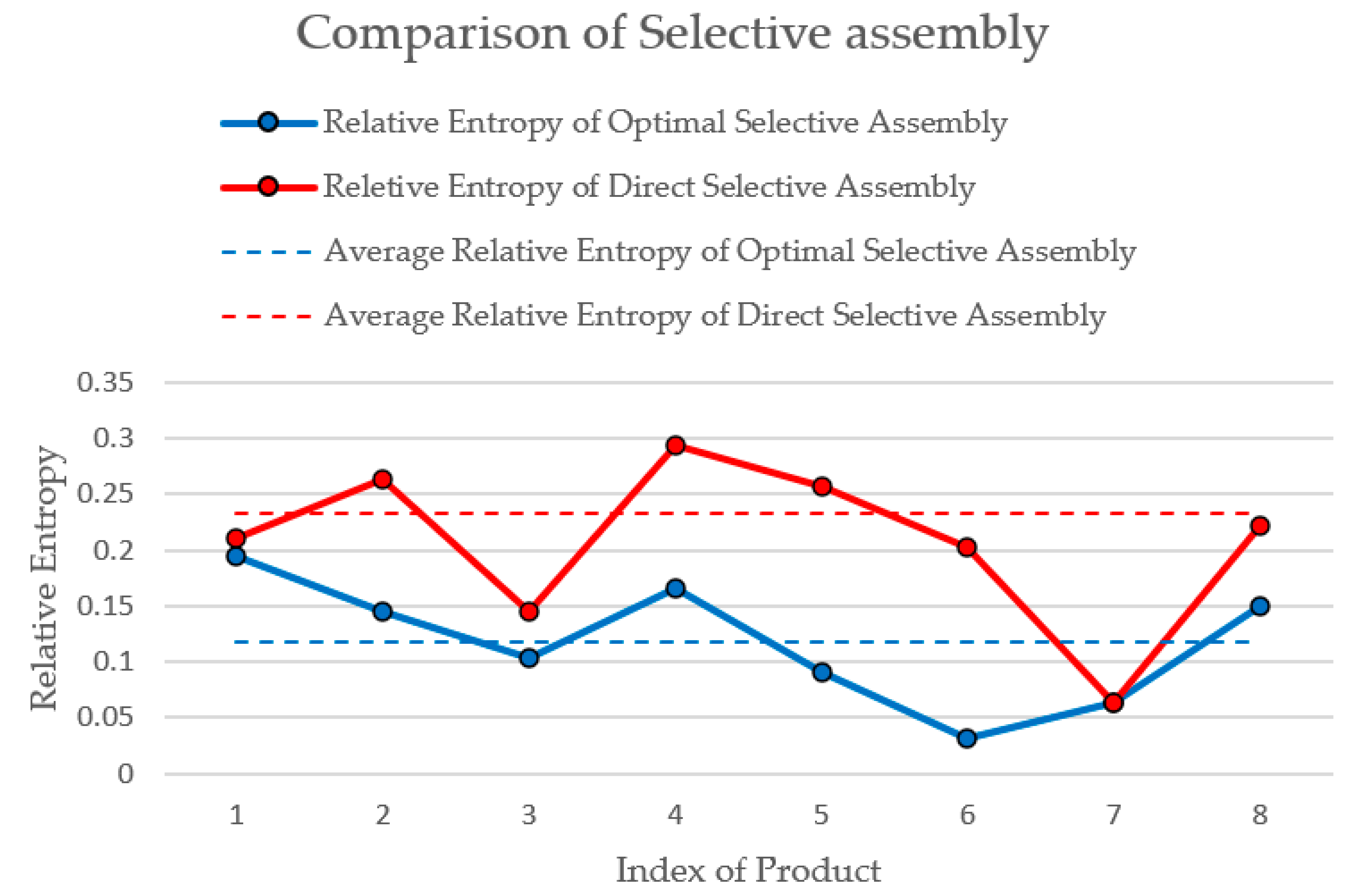
| Average relative entropy | 0.1184 | |
| Index of Shafts | Index of Holes | Relative Entropy |
|---|---|---|
| 7 | 19 | 0.0641 |
| 5 | 12 | 0.2569 |
| 3 | 6 | 0.1444 |
| 4 | 8 | 0.2938 |
| 2 | 7 | 0.2641 |
| 1 | 5 | 0.2111 |
| 8 | 17 | 0.2226 |
| 6 | 11 | 0.2023 |
| Average relative entropy | 0.2074 | |
Publisher’s Note: MDPI stays neutral with regard to jurisdictional claims in published maps and institutional affiliations. |
© 2020 by the authors. Licensee MDPI, Basel, Switzerland. This article is an open access article distributed under the terms and conditions of the Creative Commons Attribution (CC BY) license (http://creativecommons.org/licenses/by/4.0/).
Share and Cite
Xing, M.; Zhang, Q.; Jin, X.; Zhang, Z. Optimization of Selective Assembly for Shafts and Holes Based on Relative Entropy and Dynamic Programming. Entropy 2020, 22, 1211. https://doi.org/10.3390/e22111211
Xing M, Zhang Q, Jin X, Zhang Z. Optimization of Selective Assembly for Shafts and Holes Based on Relative Entropy and Dynamic Programming. Entropy. 2020; 22(11):1211. https://doi.org/10.3390/e22111211
Chicago/Turabian StyleXing, Mingyi, Qiushuang Zhang, Xin Jin, and Zhijing Zhang. 2020. "Optimization of Selective Assembly for Shafts and Holes Based on Relative Entropy and Dynamic Programming" Entropy 22, no. 11: 1211. https://doi.org/10.3390/e22111211
APA StyleXing, M., Zhang, Q., Jin, X., & Zhang, Z. (2020). Optimization of Selective Assembly for Shafts and Holes Based on Relative Entropy and Dynamic Programming. Entropy, 22(11), 1211. https://doi.org/10.3390/e22111211