Abstract
The curse of dimensionality causes the well-known and widely discussed problems for machine learning methods. There is a hypothesis that using the Manhattan distance and even fractional quasinorms (for p less than 1) can help to overcome the curse of dimensionality in classification problems. In this study, we systematically test this hypothesis. It is illustrated that fractional quasinorms have a greater relative contrast and coefficient of variation than the Euclidean norm , but it is shown that this difference decays with increasing space dimension. It has been demonstrated that the concentration of distances shows qualitatively the same behaviour for all tested norms and quasinorms. It is shown that a greater relative contrast does not mean a better classification quality. It was revealed that for different databases the best (worst) performance was achieved under different norms (quasinorms). A systematic comparison shows that the difference in the performance of kNN classifiers for at p = 0.5, 1, and 2 is statistically insignificant. Analysis of curse and blessing of dimensionality requires careful definition of data dimensionality that rarely coincides with the number of attributes. We systematically examined several intrinsic dimensions of the data.
1. Introduction
The term “curse of dimensionality” was introduced by Bellman [1] in 1957. Nowadays, this is a general term for problems related to high dimensional data, for example, for Bayesian modelling [2], nearest neighbour prediction [3] and search [4], neural networks [5,6], radial basis function networks [7,8,9,10] and many others. Many authors have studied the “meaningfulness” of distance based classification [11,12,13], clustering [12,14] and outlier detection [13,15] in high dimensions. These studies are related to the concentration of distances, which means that in high dimensional space the distances between almost all pairs of points of a random finite set have almost the same value (with high probability and for a wide class of distributions).
The term “blessing of dimensionality” was introduced by Kainen in 1997 [16]. The “blessing of dimensionality” considers the same effect of concentration of distances from the different point of view [17,18,19]. The concentration of distances was discovered in the foundation of statistical physics and analysed further in the context of probability theory [20,21], functional analysis [22], and geometry (reviewed by [23,24,25]). The blessing of dimensionality allows us to use some specific high dimensional properties to solve problems [26,27]. One such property is the linear separability of random points from finite sets in high dimensions [24,28]. A review of probability in high dimension, concentration of norm, and many other related phenomena is presented in [20].
The curse of dimensionality was firstly described 59 years ago [1] and the blessing of dimensionality was revealed 23 years ago [16]. The importance of both these phenomena increases in time. The big data revolution leads to an increase of the data dimensionality, and classical machine learning theory becomes useless in the post-classical world where the data dimensionality often exceeds the sample size (and it usually exceeds the logarithm of the sample size that makes many classical estimates pointless) [26]. The curse and blessing of dimensionality are two sides of the same coin. A curse can turn into a blessing and vice versa. For example, the recently found phenomenon of stochastic separability in high dimensions [24,29] can be considered as a “blessing” [28] because it is useful for fast non-iterative corrections of artificial intelligence systems. On the other hand, it can be considered as a “curse” [30]: the possibility to create simple and efficient correctors opens, at the same time, a vulnerability and provides tools for stealth attacks on the systems.
Since the “curse of dimensionality” and the “blessing of dimensionality” are related to the concept of high dimensionality, six different approaches to evaluation of dimension of data were taken into consideration. Beyond the usual dimension of vector space [31] (the number of atteributes), we considered three dimensions determined by linear approximation of data by principal components [32,33] with the choice of the number of principal components in accordance with the Kaiser rule [34,35], the broken stick rule [36] and the condition number of the covariance matrix [28,37]. We also considered the recently developed separability dimension [28,38] and the fractal dimension [39]. We demonstrated on many popular benchmarks that intrinsic dimensions of data are usually far from the dimension of vector space. Therefore, it is necessary to evaluate the intrinsic dimension of the data before considering any problem as high- or low-dimensional.
The functional in a d dimensional vector space is defined as
The Euclidean distance is and the Manhattan distance is . It is the norm for and the quasinorm for due to violation of the triangle inequality [40]. We consider only the case with . It is well known that for we have .
Measuring of dissimilarity and errors using subquadratic functionals reduces the influence of outliers and can help to construct more robust data analysis methods [14,41,42]. The use of these functionals for struggling with the curse of dimensionality was proposed in several works [14,42,43,44,45,46]. In particular, Aggarwal et al. [14] suggested that “fractional distance metrics can significantly improve the effectiveness of standard clustering algorithms”. Francois, Wertz, and Verleysen studied Relative Contrast (RC) and Coefficient of Variation (CV) (called by them ‘relative variance’) of distances between datapoints in different norms [42]. They found that “the ‘optimal’ value of p is highly application dependent”. For different examples, the optimal p was equal to 1, 1/2, or 1/8 [42]. Dik et al. [43] found that for fuzzy c-means usage of -quasinorms with “improves results when compared to or the usual distances, especially when there are outliers.” The purity of clusters was used for comparison. Jayaram and Klawonn [44] studied RC and CV for quasinorms without triangle inequality and for metrics unbounded on the unite cube. In particular, they found that indicators of concentration of the norm are better for lower p and, moreover, that unbounded distance functions whose expectations do not exist behave better than norms or quasinorms. France [45] compared effectiveness of several different norms for clustering. They found that the normalised metrics proposed in [46] give a better results and recommended to use the normalised metrics for nearest neighbours recovery.
In 2001, C.C. Aggarwal and co-authors [14] briefly described the effect of using fractional quasinorms for high-dimensional problems. They demonstrated that using of () can compensate the concentration of distances. This idea was used further in many works [13,47,48]. One of the main problems of using the quasinorm for is time of calculation of minimal distances and solution of optimization problems with functional (which is even non-convex for ). Several methods have been developed to speed up the calculations [47,49].
The main recommendation of [14] was the use of Manhattan distance instead of Euclidean one [50,51,52]. The main reason for this is that a smaller p is expected to give better results but for the functional is not a norm, but a non-convex quasinorm. All methods and algorithms that assume triangle inequality [51,53,54] cannot use such a quasinorm.
A comparison of different functionals for data mining problems is needed. In light of the published preliminary results, for example, [14,55,56], more testing is necessary to evaluate the performance of data mining algorithms based on these norms and quasinorms.
In our study, we perform systematic testing. In general, we demonstrated that the concentration of distances for functionals was less for smaller p. Nevertheless, for all p, the dependences of distance concentration indicators (RC and CV) on dimension are qualitatively the same. Moreover, the difference in distance concentration indicators for different p decreases with increasing dimension, both for RC and CV.
The poor performance of k Nearest Neighbour (kNN) classifiers in high dimensions is used as a standard example of the “curse of dimensionality” for a long time, from the early work [11] to the deep modern analysis [57]. The kNN classifiers are very sensitive to used distance (or proximity) functions and, therefore, they are of particular interest to our research.
We have systematically tested the hypothesis that measuring of dissimilarity by subquadratic norms or even quasinorms can help to overcome the curse of dimensionality in classification problems. We have shown that these norms and quasinorms do not systematically and significantly improve performance of kNN classifiers in high dimensions.
In addition to the main result, some simple technical findings will be demonstrated below that can be useful when analyzing multivariate data. Two of them are related to the estimation of the dimension of the data, and the other two consider the links between the use of different norms, the concentration of distances and the accuracy of the kNN classifiers:
- The number of attributes for most of real life databases is far from any reasonable intrinsic dimensionality of data;
- The popular estimations of intrinsic dimensionality based on principal components (Kaiser rule and broken stick rule) are very sensitive to irrelevant attributes, while the estimations based on the condition number of the reduced covariance matrix is much more stable as well as the definitions based on separability properties or fractal dimension;
- Usage of functionals with small p does not prevent the concentration of distances;
- A lower value of a distance concentration indicator does not mean better accuracy of the kNN classification.
Our paper is organized as follows. In Section 2, we present results of an empirical test of distance concentration for relative contrast and coefficient of variation also known as relative variance. Section 3 introduces the six used intrinsic dimensions. In Section 4, we describe the approaches used for functionals comparison, the used databases and the classification quality indicators. In Section 5, six intrinsic dimensions are compared for the benchmark datasets. In Section 6, we compare performance of classifiers for different functionals. The ‘Discussion’ section provides discussion and outlook. The ‘Conclusion’ section presents conclusions.
2. Measure Concentration
Consider a database X with n data points and d real-valued attributes, . x without index is the query point: the point for which all distances were calculated. We used for testing two types of databases: randomly generated databases with i.i.d. components from the uniform distribution on the interval (this section) and real life databases (Section 4). The functional for vector x is defined by (1). For comparability of results with [14], in this study, we consider the set of norms and quasinorms used in [14] with one more quasinorm (): .
Figure 1 shows the shapes of the unit level sets for all considered norms and quasinorms excluding and . For two excluded quasinorms, the level sets are visually indistinguishable from the central cross.
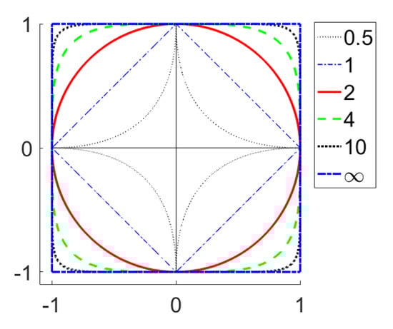
Figure 1.
Unit level sets for functionals (“Unit spheres”).
Several different indicators were used to study the concentration of distances:
- Relative Contrast (RC) [11,14,42]
- Coefficient of Variations (CV) or relative variance [42,53,54]where is the variance and is the mean value of the random variable z;
- Hubness (popular nearest neighbours) [13].
In our study, we used RC and CV. Hubness [13] characterised distribution of the number of k-occurrences of data points that is, the number of times the data point occurs among the k nearest neighbours of all other data points. With dimensionality increase, the distribution this k-occurrence becomes more skewed to the right, that indicates the emergence of hubs, i.e., popular nearest neighbours which appear in many more kNN lists than other points. We did not use hubness in our analysis because this change in the distribution of a special random variable, k-occurrence, needs additional convention about interpretation. Comparison of distributions is not so illustrative as comparison of real numbers.
Table 2 in paper [14] shows that the proportion of cases where increases with dimension. It can be easily shown that for special choice of X and x, all three relations between RC and RC are possible: (all lines in Figure 2, exclude row 6), , or (row 6 in Figure 2). To evaluate the probabilities of these three outcomes, we performed the following experiment. We generated X dataset with k points and 100 coordinates. Each coordinate of each point was uniformly randomly generated in the interval . For each dimension , we created a d-dimensional dataset by selecting the first d coordinates of points in X. We calculated as the mean value of RC for each point in :
where is the X database without the point x. We repeated this procedure 1000 times and calculated the fraction of cases when . The results of this experiment are presented in Table 1. Table 1 shows that for points our results are very similar to the results presented in Table 2 in [14]. Increasing the number of points shows that even with a relatively small number of points () for almost all databases .
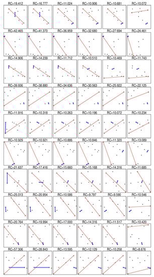
Figure 2.
Ten randomly generated sets of 10 points, thin red line connects the furthest points and bold blue line connects closest points, columns (from left to right) corresponds to .

Table 1.
Comparison of RC for and for different dimension of space (Dim) and different number of points.
We can see that appearance of a noticeable proportion of cases when is caused by a small sample size. For not so small samples, in most cases . This is mainly because the pairs of nearest (farthest) points can be different for different metrics. Several examples of such sets are presented in Figure 2. Figure 2 shows that in rows 3, 5, 6, and 8 and in row 6. These results allow us to formulate the hypothesis that in general almost always . RC is widely used to study the properties of a finite set of points, but CV is more appropriate for point distributions. We hypothesise that .
To check these hypotheses, we performed the following experiment. We created a X database with 10,000 points in 200 dimensional space. Each coordinate of each point was uniformly randomly generated in the interval . We chose the set of dimensions and the set of functionals . For each dimension d, we prepared the database as the set of the first d coordinates of points in X database. For each database and functional, we calculate the set of all pairwise distances . Then, we estimated the following values:
The graphs and are presented in Figure 3. Figure 3 shows that our hypotheses hold. We see that RC and CV as functions of dimension have qualitatively the same shape but in different scales: RC in the logarithmic scale. The paper [14] states that the qualitatively different behaviour of was observed for different p. We found qualitatively the same behavior for relative values (RC). The small quantitative difference increases for d from 1 to about 10 and decreases with a further increase in dimension. This means that there could be some preference for using lower values of p but the fractional metrics do not provide a panacea for the curse of dimensionality. To analyse this hypothesis, we study the real live benchmarks in the Section 4.
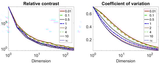
Figure 3.
Changes of RC (left) and CV (right) with dimension for several metrics.
3. Dimension Estimation
To consider high dimensional data and the curse or blessing of dimensionality, it is necessary to determine what dimensionality is. There are many different notions of data dimension. Evaluation of dimensionality become very important with emergence of many “big data” databases. The number of attributes is the dimension of the vector space [31] (hereinafter referred to as #Attr). For the data mining tasks, the dimension of space is not as important as the data dimension and the intrinsic data dimension is usually less than the dimension of space.
The concept of intrinsic, internal or effective data dimensionality is not well defined for the obvious reason: the data sets are finite and, therefore, the direct application of topological definitions of dimension gives zero. The most popular approach to determining the data dimensionality is approximation of data sets by a continuous topological object. Perhaps, the first and at the same time widely used definition of intrinsic dimension is the dimension of the linear manifold of “the best fit to data” with sufficiently small deviations [32]. The simplest way to evaluate such dimension is Principal Component Analysis (PCA) [32,33]. There is no single (unambiguous) method for determining the number of informative (important, relevant, etc.) principal components [36,60,61]. The two widely used methods are the Kaiser rule [34,35] (hereinafter referred to as PCA-K) and the broken stick rule [36] (hereinafter referred to as PCA-BS).
Let us consider a X database with n data points and d real-valued attributes, . The empirical covariance matrix is symmetric and non-negative definite. The eigenvalues of the matrix are non-negative real numbers. Denote these values as . Principal components are defined using the eigenvectors of empirical covariance matrix . If the ith eigenvector is defined then the ith principal coordinate of the datavector x is the inner product . The Fraction of Variance Explained (FVE) by ith principal component for the dataset X is
The Kaiser rule states that all principal components with FVE greater or equal to the average FVE are informative. The average FVE is . Thus, the components with are considered as informative ones and should be retained and the components with should not. Another popular version uses a twice lower threshold and retains more components.
The broken stick rule compares the set with the distribution of random intervals that appear if we break the stick at points randomly and independently sampled from the uniform distribution. Consider a unit interval (stick) randomly broken into d fragments. Let us numerate these fragments in descending order of their length: . Expected length of i fragment is [36]
The broken stick rule states that the first k principal components are informative, where k is the maximum number such that .
In many problems, the empirical covariance matrix degenerates or almost degenerates, that means that the smallest eigenvalues are much smaller than the largest ones. Consider the projection of data on the first k principal components: , where the columns of the matrix V are the first k eigenvectors of the matrix . Eigenvalues of the empirical covariance matrix of the reduced data are . After the dimensionality reduction, the condition number (the ratio of the lowest eigenvalue to the greatest) [62] of the reduced covariance matrix should not be too high in order to avoid the multicollinearity problem. The relevant definition [28] of the intrinsic dimensionality refers directly to the condition number of the matrix : k is the number of informative principal components if it is the smallest number such that
where C is specified condition number, for example, . This approach is further referred to as PCA-CN. The PCA-CN intrinsic dimensionality is defined as the number of eigenvalues of the covariance matrix exceeding a fixed percent of its largest eigenvalue [37].
The development of the idea of data approximation led to the appearance of principal manifolds [63] and more sophisticated approximators, such as principal graphs and complexes [64,65]. These approaches provide tools for evaluating the intrinsic dimensionality of data and measuring the data complexity [66]. Another approach uses complexes with vertices in data points: just connect the points with distance less than for different and get an object of combinatorial topology, simplicial complex [67]. All these methods use an object embedded in the data space. They are called Injective Methods [68]. In addition, a family of Projective Methods was developed. These methods do not construct a data approximator, but project the dataspace onto a space of lower dimension with preservation of similarity or dissimilarity of objects. A brief review of modern injective and projective methods can be found in [68].
Recent studies of curse/blessing dimensionality introduce a new method for evaluation intrinsic dimension: separability analysis. A detailed description of this method can be found in [28,38] (hereinafter referred to as SepD). For this study, we used an implementation of separability analysis from [69]. The main concept of this approach is the Fisher separability: point x of dataset X is Fisher separable from dataset X if
where is dot product of vectors x and y.
The last intrinsic dimension used in this study is the fractal dimension (hereinafter referred to as FracD). It is also known as box-counting dimension or Minkowsk–Bouligand dimension. There are many versions of box-counting algorithms and we used R implementation from the RDimtools package [70]. The definition of FracD is
where r is the size of the d-cubic box in the regular grid and is the number of cells with data points in this grid. Of course, formally this definition is controversial since the data set is finite and there is no infinite sequence of discrete sets. In practice, the limit is substituted by the slope of the linear regression for sufficiently small r but without intercept.
There are many approaches to non-linear evaluation of data dimensionality with various non-linear data approximants: manifolds, graphs or cell complexes [63,65,66,68]. The technology of neural network autoencoders is also efficient and very popular but its theoretical background is still under discussion [71]. We did not include any other non-linear dimensionality reduction methods in our study because there is a fundamental uncertainty: it is not known a priori when to stop the reduction. Even for simple linear PCA, we have to consider and compare three stopping criteria, from Kaiser rule to the condition number restriction. For non-linear model reduction algorithms the choice of possible estimates and stopping criteria is much richer. The non-linear estimates of the dimensionality of data may be much smaller than the linear ones. Nevertheless, for the real life biomedical datasets, the difference between linear and non-linear dimensions is often not so large (from 1 to 4), as it was demonstrated in [65].
4. Comparison of lp Functionals
In Section 2, we demonstrated that is greater for smaller p. It was shown in [11] that greater RC means ‘more meaningful’ task for kNN. We decided to compare different functions for kNN classification. Classification has one additional advantage over regression and clustering problems: the standard criteria of classification quality are classifier independent and and do not depend on the dissimilarity measures used [72].
For this study, we selected three classification quality criteria: the Total Number of Neighbours of the Same Class (TNNSC) (that is, the total number of the k nearest neighbors that belonged to the same class as the target object over all the different target objects), accuracy (fraction of correctly recognised cases), sum of sensitivity (fraction of correctly solved cases of positive class) and specificity (fraction of correctly solved cases of negative class). TNNSC is not an obvious indicator of classification quality and we use it for comparability of our results with [14]. kNN with 11 nearest neighbours was used also for comparability with [14].
4.1. Databases for Comparison
We selected 25 databases from UCI Data repository [73]. To select the databases, we applied the following criteria:
- Data are not time-series.
- Database is formed for the binary classification problem.
- Database does not contain any missing values.
- The number of attributes is less than the number of observations and is greater than 3.
- All predictors are binary or numeric.
In total, 25 databases and 37 binary classification problems were selected (some databases contain more than one classification problem). For simplicity, we refer to each task as a ‘database’. The list of selected databases is presented in Table 2.
Table 2.
Databases selected for analysis.
We do not set out to determine the best database preprocessing for each database. We just use three preprocessing for each database:
- Empty preprocessing means usage data ‘as is’;
- Standardisation means shifting and scaling data to have a zero mean and unit variance;
- Min-max normalization refers to shifting and scaling data in the interval .
4.2. Approaches to Comparison
Our purpose is to compare functionals but not to create the best classifier for each problem. Following [14], we use the 11NN classifier, and 3NN, 5NN and 7NN classifiers for more general result. One of the reasons for choosing kNN is strong dependence of kNN on used metrics and, on the other hand, the absence of any assumption about the data, excluding the principle: tell me your neighbours, and I will tell you what you are. In our study, we consider kNN with as different algorithms. We applied the following indicators to compare kNN classifiers (algorithms) for listed functionals:
- The number of databases for which the algorithm is the best [107];
- The number of databases for which the algorithm is the worst [107];
- The number of databases for which the algorithm has performance that is statistically insignificantly different from the best;
- The number of databases for which the algorithm has performance that is statistically insignificantly different from the worst;
- The Friedman test [108,109] and post hoc Nemenyi test [110] which were specially developed to compare multiple algorithms;
- The Wilcoxon signed rank test was used to compare three pairs of metrics.
We call the first four approaches frequency comparison. To avoid discrepancies, a description of all used statistical tests is presented below.
4.2.1. Proportion Estimation
Since two criteria of classification quality – accuracy and , where n is the number of cases in the database – are proportions, we can apply z-test for proportion estimations [111]. We want to compare two proportions with the same sample size, so we can use a simplified formula for test statistics:
where and are two proportions for comparison. p-value of this test is the probability of observing by chance the same or greater z if both samples are taken from the same population. p-value is , where is the standard cumulative normal distribution. There is a problem of reasonable choice of significance level. The selected databases contain from 90 to 130,064 cases. Using the same threshold for all databases is meaningless [112,113]. The required sample size n can be estimated through the specified significance level of , the statistical power , the expected effect size e, and the population variance . For the normal distribution (since we use z-test) this estimation is:
In this study, we assume that the significance level is equal to the statistical power , the expected effect size is 1% (1% difference in accuracy is large enough), and the population variance can be estimated by the formula
where is the number of cases in the positive class. Based on this assumption, we can estimate a reasonable level of significance as
Usage of eight functionals means multiple testing. To avoid overdetection problem we apply Bonferroni correction [114]. On the other hand, usage of too high a significance level is also meaningless [112]. As a result, we select the significance level as
The difference between two proportions (TNNSC or accuracy) is statistically significant if . It must be emphasized that for TNNSC the number of cases is because we consider k neighbours for each point.
4.2.2. Friedman Test and Post Hoc Nemenyi Test
One of the widely used statistical tests for comparing algorithms on many databases is the Friedman test [108,109]. To apply this test, we firstly need to apply the tied ranking for the classification quality score for one database: if several classifiers provide exactly the same quality score then the rank of all such classifiers will be equal to the average value of the ranks for which they were tied [109]. We denote the number of used databases as N, the number of used classifiers as m and the rank of classifier i for database j as . The mean rank of classifier i is
Test statistics is
Test statistics under null hypothesis that all classifiers have the same performance follows the distribution with degrees of freedom. p-value of this test is the probability of observing by chance the same or greater if all classifiers have the same performance. p-value is , where is the cumulative distribution with degrees of freedom. Since we only have 37 databases, we decide to use the 95% significance level.
If the Friedman test shows enough evidence to reject the null hypothesis, then we can conclude that not all classifiers have the same performance. To identify pairs of classifiers with significantly different performances, we applied the post hoc Nemenyi test [110]. Test statistics for comparing of classifiers i and j is . To identify pairs with statistically significant differences the critical distance
is used. Here, is the critical value for the Nemenyi test with a significance level of and m degrees of freedom. The difference of classifiers performances is statistically significant with a significance level of if .
4.2.3. Wilcoxon Signed Rank Test
To compare the performance of two classifiers on several databases we applied the Wilcoxon signed rank test [115]. For this test we used the standard Matlab function signrank [116].
5. Dimension Comparison
An evaluation of six dimensions, number of attributes (dimension of space) and five intrinsic dimensions of data, for benchmarks is presented in Table 2. It can be seen, that for each considered intrinsic dimension of data, this dimension does not grow monotonously with the number of attributes for the given set of benchmarks. The correlation matrix of all six dimensions is presented in Table 3. There are two groups of highly correlated dimensions:
Table 3.
Correlation matrix for six dimensionality: two groups of highly correlated dimensions are highlighted by the background colours.
- #Attr, PCA-K and PCA-BS;
- PCA-CN and SepD.
Correlations between groups are low (the maximum value is 0.154). The fractal dimension (FracD) is correlated (but is not strongly correlated) with PCA-CN and SepD.
Consider the first group of correlated dimensions. Linear regressions of PCA-K and PCA-BS on #Attr are
It is necessary to emphasize that a coefficient 0.29 (0.027 for PCA-BS) was determined only for datasets considered in this study and can be different for another datasets, but multiple R squared equals 0.998 (0.855 for PCA-BS), shows that this dependence is not accidental. What is the reason for the strong correlations of these dimensions? It can be shown that these dimensions are sensitive to irrelevant or redundant attributes. The simplest example is adding highly correlated attributes. To illustrate this property of these dimensions, consider an abstract database X with d standardised attributes and a covariance matrix . This covariance matrix has d eigenvalues and corresponding eigenvectors . To determine the PCA-K dimension, we must compare FVE of each principal component with the threshold . Since all attributes are standardized, the elements of the main diagonal of the matrix are equal to one. This means that and the FVE of i principal component is .
Consider duplication of attributes: add copies of the original attributes to the data table. This operation does not add any information to the data and, in principle, should not affect the intrinsic dimension of the data for any reasonable definition.
Denote all object for this new database by superscript . The new dataset is , where symbol | denotes the concatenation of two row vectors. For any data vectors and , the dot product is .
For a new dataset the covariance matrix has the form
The first d eigenvectors can be represented as , where ⊺ means transposition of the matrix (vector). Calculate the product of and :
As we can see, each of the first d eigenvalues become twice as large (). This means that the FVE of the first d principal components have the same values
Since sum of the eigenvalues of the matrix is , we can conclude that . We can repeat the described procedure for copying attributes several times and determine the values and , where m is the number of copies of attributes added. For the database , the informativeness threshold of principal components is . Obviously, for any nonzero eigenvalue , there exists m such that . This means that trivial operation of adding copies of attributes can increase informativeness of principal components and the number of informative main components or PCA-K dimension.
To evaluate the effect of the attribute copying procedure on the broken stick dimension, the following two propositions are needed:
Proposition 1.
If , then and .
Proposition 2.
If , then and .
Proofs of these propositions are presented in Appendix A.
The simulation results of process of the attribute copying for ‘Musk 1’ and ‘Gisette’ databases are presented in Table 4.
Table 4.
Attribute duplication process for ‘Musk 1’ and ‘Gisette’ databases.
Now we are ready to evaluate the effect of duplication of attributes on the dimensions under consideration, keeping in mind that nothing should change for reasonable definitions of data dimension.
- The dimension of the vector space of the dataset is (see Table 4).
- For the dimension defined by the Kaiser rule, PCA-K, the threshold of informativeness is . This means that for all principal components with nonzero eigenvalues, we can take large enough m to ensure that these principal components are “informative” (see Table 4). The significance threshold decreases linearly with increasing m.
- For the dimension defined by the broken stick rule, PCA-BS, we observe initially an increase in the thresholds for the last half of the original principal components, but then the thresholds decrease with an increase in m for all . This means that for all principal components with nonzero eigenvalues, we can take large enough m to ensure that these principal components are “informative” (see Table 4). The thresholds of significance decrease non-linearly with increasing m. This slower than linear thresholds decreasing shows that PCA-BS is less sensitivity to irrelevant attributes than #Attr or PCA-K.
- For the PCA-CN dimension defined by condition number, nothing changes in the described procedure since simultaneous multiplying of all eigenvalues by a nonzero constant does not change the fraction of eigenvalues in the condition (7).
- Adding irrelevant attributes does not change anything for separability dimension, SepD, since the dot product of any two data points in the extended database is the dot products of the corresponding vectors in the original data set multiplied by . This means that described extension of dataset change nothing in the separability inequality (8).
- There are no changes for the fractal dimension FracD, since the described extension of dataset does not change the relative location of data points in space. This means that values will be the same for original and extended datasets.
The second group of correlated dimensions includes PCA-CN, SepD, and FracD. The first two are highly correlated and the last one is moderately correlated with the first two. Linear regressions of these dimensions are
High correlation of these three dimensions requires additional investigations.
6. Results of lp Functionals Comparison
The results of a direct comparison of the algorithms are presented in Table 5 for 11NN, Table A1 for 3NN, Table A2 for 5NN, and Table A3 for 7NN. Table 5 shows that ‘The best’ indicator is not reliable and cannot be considered as a good tool for performance comparison [107]. For example, for TNNSC with empty preprocessing, is the best for 11 databases and this is the maximal value, but and are essentially better if we consider indicator ‘Insignificantly different from the best’: 26 databases for and 31 databases for and . This fact confirms that the indicator ‘Insignificantly different from the best’ is more reliable. Analysis of Table 5 shows that on average and are the best and and are the worst. Qualitatively the same results are contained in Table A1 for 3NN, Table A2 for 5NN, and Table A3 for 7NN
Table 5.
Frequency comparison for TNNSC, accuracy and sensitivity plus specificity, 11NN.
The results of the Friedman and post hoc Nemenyi tests are presented in Table 6, Table 7, Table 8 and Table 9. We applied these tests for three different preprocessings and three classification quality indicators. In total, we tested nine sets for eight algorithms and 37 databases. Tests was performed for kNN with . The post hoc Nemenyi test was used to define algorithms with performance that do not significantly differ from the best algorithm. It can be seen that is the best for 50% tests (18 of 36 sets), is the best for 42% of tests (15 of 36 sets), and is the best for 8% of tests (3 of 36 sets). On the other hand, performances of and are insignificantly different from the best for all nine sets and all four kNN.
Table 6.
Results of the Friedman test and post hoc Nemenyi test, 11NN.
Table 7.
Results of the Friedman test and post hoc Nemenyi test, 3NN.
Table 8.
Results of the Friedman test and post hoc Nemenyi test, 5NN.
Table 9.
Results of the Friedman test and post hoc Nemenyi test, 7NN.
We compared eight different functionals on 37 databases. The authors of [14] have hypothesised that: (i) kNN based on is better than based on and (ii) that the “fractional” metrics can further improve performance. We tested the differences between 11NN classifiers based on and by direct usage of Wilcoxon test. This comparison does not take into account the multiple testing. The results of comparisons are presented in Table 10 and Table 11. The top table shows that in all cases kNN based on and have insignificantly different performances and for the most cases kNN based on is slightly worse than the previous two. The bottom table shows, that kNN based on and are insensitive to type of preprocessing (the performances of both methods are not significantly different for different preprocessing). In contrast to these two methods, kNN based on shows significantly better performance for min-max normalization preprocessing in comparison with two other preprocessings (p-values for both tests are less than 1%).
Table 10.
p-values of Wilcoxon test for different functions: Se+Sp stands for sensitivity plus specificity.
Table 11.
p-values of Wilcoxon test for different type of preprocessing (bottom): E for empty preprocessing, S for standardisation, and M for min-max normalization preprocessing, and Se+Sp stands for sensitivity plus specificity.
7. Discussion
In this paper, we tested the rather popular hypothesis that using the norms with (preferably ) or even the quasinorm with helps to overcome the curse of dimensionality.
Traditionally, the first choice of test datasets for analysing the curse or blessing of dimensionality is to use samples from some simple distributions: uniform distributions on the balls, cubes, other convex compacts, or normal distributions (see, for example, [4,11,12,13,14,15,18], etc.). Further, generalisations are used such as the product of distributions in a cube (instead of uniform distributions) or log-concave distributions (instead of normal distributions) [28,117,118]. For such distributions was proven properties of data concentration in thin layer [117], and further in waists of such layers [22]. We used data sampled from the uniform distribution on the unit cube to analyse the distribution of distances in high dimensions for various p. To assess the impact of dimension on classification, we used collection of 25 datasets from different sources (Table 2). The number of attributes in these databases varies from 4 to 5000.
For real-life datasets, the distributions are not just unknown—there is doubt that the data are sampled from a more or less regular distribution. Moreover, we cannot always be sure that the concepts of probability distribution and statistical sampling are applicable. If we want to test any hypothesis about the curse or blessing of dimensionality and methods of working with high-dimensional data, then the first problem we face is: what is data dimensionality? Beyond hypotheses about regular distribution, we cannot blindly assume that the data dimensionality is the same as the number of attributes. Therefore, the first task was to evaluate the intrinsic dimension of all the data sets selected for testing.
Five dimensionalities of data were considered and compared:
- PCA with Kaiser rule for determining the number of principal components to retain (PCA-K);
- PCA with the broken stick rule for determining the number of principal components to retain (PCA-BS);
- PCA with the condition number criterion for determining the number of principal components to retain (PCA-CN);
- The Fisher separability dimension (SepD);
- The fractal dimension (FracD).
We demonstrated that both the Kaiser rule (PCA-K) and the broken stick rule (PCA-BS) are very sensitive to the addition of attribute duplicates. It can be easily shown that these dimensions are also very sensitive to adding of highly correlated attributes. In particular, for these rules, the number of informative principal components depend on the ‘tail’ of the minor components.
The condition number criterion (PCA-CN) gives much stabler results. The dimensionality estimates based on the fundamental topological and geometric properties of the data set (the Fisher separability dimension, SepD, and the fractal dimension, FracD) are less sensitive to adding highly correlated attributes and insensitive to duplicate attributes.
Dimensions PCA-K and PCA-BS are strongly correlated () for the selected set of benchmarks. Their correlations with the number of attributes are also very strong (Table 3). The correlations of these dimensions with three other dimensions (PCA-CN, SepD, and FracD) are essentially weaker. Dimensions PCA-CN and SepD are also strongly correlated (), and their correlations with FracD are moderate (see Table 3).
The results of testing have convinced us that the PCA-CN and SepD estimates of the intrinsic dimensionality of the data are more suitable for practical use than the PCA-K and PCA-BS estimates. The FracD estimate is also suitable. A detailed comparison with many other estimates is beyond the scope of this paper.
The choice of criteria is very important for identifying the advantages of using non-Euclidean norms and quasi-norms (). RC (2) and CV (3) of high dimensional data are widely used for this purposes. In some examples (see [12,14]) it was demonstrated that for norms or quasinorms, the RC decreases with increasing dimension. It was also shown [14] that RC for functionals with lower p are greater than for functionals with greater p (see Figure 3).
Our tests for data sets sampled from a regular distribution (uniform distribution in a cube) confirm this phenomenon. However Figure 3 shows that decreasing of p cannot compensate (improve) the curse of dimensionality: the RC for high dimensional data and small p will be less than for usual Euclidean distance in some lower dimensional space. The behavior of a CV with a change in dimension is similar to that of RC. In our experiments, the inequalities and were almost always satisfied. We found that the differences in RC and CV for different p decay with dimension tends to infinity.
Authors of [14] stated that “fractional distance metrics can significantly improve the effectiveness of standard clustering algorithms”. In contrast, our tests on the collection of the benchmark datasets showed that there is no direct relationship between the distance concentration indicators (e.g., RC or CV) and the quality of classifiers: kNN based on has one of the worst classification performance but the greatest and . Comparison of the classification quality of 3NN, 5NN, 7NN and 11NN classifiers for different functionals and for different databases shows that the greater RC does not mean the higher quality.
The authors of [14] found that “is consistently more preferable than the Euclidean distance metric for high dimensional data mining applications”. Our study partially confirmed the first finding: kNN with distance often shows better performance compared to but this difference is not always statistically significant.
Finally, the performance of kNN classifiers based on and functionals is statistically indistinguishable for .
A detailed pairwise comparison of the , and functions shows that the performance of a based kNN is more sensitive to the preprocessing used than a and based kNN. There is no unique and unconditional leader among the functionals for classification problems. We can conclude that the based kNN classifiers with very small and very big are almost always worse than with intermediate p, . Our massive test shows that for all preprocessing used and all considered classifier quality indicators, the performance of kNN classifiers based on for , and does not differ statistically significantly.
In regards to the estimation of dimensions, the question is: can the number of based major principal components be considered as a reasonable estimate of the “real” data dimension or it is necessary to use based PCA? Recently developed PQSQ PCA [49] gives the possibility to create PCA with various subquadratic functionals, including for . The question about performance of clustering algorithms with different functionals remains still open. This problem seems less clearly posed than for supervised classification, since there are no unconditional criteria for “correct clustering” (or too many criteria that contradict each other), as is expected for unsupervised learning.
8. Conclusions
Thus, after detailed discussion, we have to repeat the title “Fractional norms and quasinorms do not help to overcome the curse of dimensionality“. The ‘champion’ norms for the kNN classification are not far from the classical and norms. We did not find any evidence that it is more efficient to use in classification norms with or .
What do all these results mean for the practice of data mining? The fist answer is: we have to trust in classical norms more. If there are no good classifiers with the classical norms and , then class separability is likely to be unsatisfactory in other norms. Feature selection and various dimensionality reduction techniques are potentially much more powerful in improving classification than playing with norms.
Of course, without any hypothesis about data distribution such an advice cannot be transformed into a theorem, but here we would like to formulate a hypothesis that for sufficiently regular distributions in classes, the performance of kNN classifiers in high dimensions is asymptotically the same for different norms.
What can we say about other data mining problems? We cannot be sure a priori that the change of norm will not help. Nevertheless, the geometric measure concentration theorems give us a hint that for sufficiently high dimensionality of data the difference between the methods that use different norms will vanish.
Of course, this advice also has limitations. There are some obvious differences between norms. For example, partial derivatives of and norms differ significantly at zeros of coordinate . This difference was utilised, for example, in lasso methods to obtain sparse regression [119]. These properties are not specific for high dimension.
Author Contributions
Conceptualization, A.G. and E.M.M.; methodology, E.M.M. and A.G.; software, E.M.M. and J.A.; validation, A.G., E.M.M. and J.A.; formal analysis, J.A.; data curation, E.M.M. and J.A.; writing—original draft preparation, E.M.M.; writing—review and editing, E.M.M., J.A. and A.G.; visualization, E.M.M. and J.A.; supervision, A.G.; funding acquisition, A.G. All authors have read and agreed to the published version of the manuscript.
Funding
Supported by the University of Leicester, UK, EMM and ANG were supported by the Ministry of Science and Higher Education of the Russian Federation, project number 14.Y26.31.0022, JA was supported by the Taibah University, Saudi Arabia.
Conflicts of Interest
The authors declare no conflict of interest.
Abbreviations
The following abbreviations are used in this manuscript:
| kNN | k nearest neighbours |
| RC | relative contrast |
| CV | coefficient of variation |
| #Attr | the number of attributes or Hamel dimension |
| PCA | principle component analysis |
| PCA-K | dimension of space according to Kaiser rule for PCA |
| PCA-BS | dimension of space according to broken stick rule for PCA |
| FVE | fraction of variance explained |
| PCA-CN | dimension of space defined by condition number for PCA |
| SepD | dimension of space defined according to separability theorem |
| FracD | intrinsic dimension defined as fractal dimension |
| TNNSC | total number of neighbours of the same class in nearest neighbours of all points |
| Se | sensitivity or fraction of correctly recognised cases of positive class |
| Sp | specificity or fraction of correctly recognised cases of negative class |
Appendix A. Proof of Propositions
Proposition 1.
If , then and .
Proof.
Proposition 2.
If , then and .
Proof.
Appendix B. Results for kNN Tests for k = 3, 5, 7
Table A1.
Frequency comparison for TNNSC, accuracy and sensitivity plus specificity, 3NN.
Table A1.
Frequency comparison for TNNSC, accuracy and sensitivity plus specificity, 3NN.
| Indicator\p for Functional | 0.01 | 0.1 | 0.5 | 1 | 2 | 4 | 10 | ∞ |
|---|---|---|---|---|---|---|---|---|
| TNNSC | ||||||||
| Empty preprocessing | ||||||||
| The best | 3 | 10 | 11 | 1 | 7 | 2 | 0 | 3 |
| Insignificantly different from the best | 23 | 28 | 31 | 32 | 32 | 30 | 27 | 25 |
| The worst | 20 | 4 | 1 | 1 | 1 | 4 | 4 | 9 |
| Insignificantly different from the worst | 32 | 25 | 23 | 23 | 24 | 25 | 26 | 26 |
| Standardisation | ||||||||
| The best | 1 | 4 | 9 | 7 | 8 | 2 | 3 | 2 |
| Insignificantly different from the best | 23 | 28 | 32 | 33 | 32 | 31 | 29 | 26 |
| The worst | 17 | 1 | 0 | 0 | 0 | 2 | 4 | 11 |
| Insignificantly different from the worst | 34 | 27 | 26 | 24 | 24 | 25 | 25 | 26 |
| Min-max normalization | ||||||||
| The best | 2 | 4 | 5 | 10 | 8 | 3 | 1 | 6 |
| Insignificantly different from the best | 18 | 25 | 31 | 30 | 28 | 28 | 25 | 26 |
| The worst | 21 | 3 | 2 | 4 | 2 | 3 | 3 | 8 |
| Insignificantly different from the worst | 33 | 24 | 24 | 22 | 21 | 23 | 26 | 27 |
| Accuracy | ||||||||
| Empty preprocessing | ||||||||
| The best | 2 | 11 | 10 | 2 | 8 | 1 | 1 | 2 |
| Insignificantly different from the best | 26 | 31 | 33 | 34 | 34 | 33 | 33 | 32 |
| The worst | 17 | 4 | 1 | 3 | 1 | 3 | 8 | 7 |
| Insignificantly different from the worst | 34 | 28 | 28 | 27 | 26 | 28 | 29 | 29 |
| Accuracy | ||||||||
| Standardisation | ||||||||
| The best | 0 | 4 | 12 | 8 | 8 | 2 | 3 | 2 |
| Insignificantly different from the best | 26 | 30 | 34 | 33 | 33 | 33 | 30 | 30 |
| The worst | 15 | 2 | 0 | 0 | 2 | 3 | 6 | 8 |
| Insignificantly different from the worst | 34 | 29 | 28 | 27 | 27 | 28 | 29 | 29 |
| Min-max normalization | ||||||||
| The best | 2 | 4 | 9 | 13 | 6 | 4 | 1 | 6 |
| Insignificantly different from the best | 27 | 29 | 33 | 32 | 32 | 31 | 31 | 31 |
| The worst | 15 | 4 | 5 | 4 | 3 | 4 | 5 | 9 |
| Insignificantly different from the worst | 34 | 30 | 27 | 28 | 29 | 29 | 30 | 29 |
| Sensitivity plus specificity | ||||||||
| Empty preprocessing | ||||||||
| The best | 5 | 11 | 9 | 4 | 8 | 2 | 2 | 1 |
| The worst | 14 | 2 | 1 | 2 | 0 | 2 | 6 | 9 |
| Standardisation | ||||||||
| The best | 1 | 7 | 10 | 5 | 8 | 2 | 2 | 3 |
| The worst | 12 | 1 | 0 | 1 | 2 | 2 | 7 | 10 |
| Min-max normalization | ||||||||
| The best | 4 | 6 | 9 | 13 | 6 | 4 | 4 | 2 |
| The worst | 14 | 1 | 2 | 3 | 2 | 2 | 5 | 11 |
Table A2.
Frequency comparison for TNNSC, accuracy and sensitivity plus specificity, 5NN.
Table A2.
Frequency comparison for TNNSC, accuracy and sensitivity plus specificity, 5NN.
| Indicator\p for functional | 0.01 | 0.1 | 0.5 | 1 | 2 | 4 | 10 | ∞ |
|---|---|---|---|---|---|---|---|---|
| TNNSC | ||||||||
| Empty preprocessing | ||||||||
| The best | 2 | 9 | 7 | 3 | 7 | 3 | 2 | 2 |
| Insignificantly different from the best | 21 | 28 | 31 | 32 | 32 | 28 | 25 | 22 |
| The worst | 20 | 2 | 1 | 1 | 1 | 3 | 2 | 10 |
| Insignificantly different from the worst | 31 | 24 | 20 | 22 | 23 | 24 | 25 | 26 |
| Standardisation | ||||||||
| The best | 0 | 3 | 10 | 9 | 9 | 1 | 2 | 3 |
| Insignificantly different from the best | 20 | 28 | 32 | 32 | 31 | 31 | 28 | 25 |
| The worst | 20 | 1 | 1 | 2 | 0 | 1 | 2 | 10 |
| Insignificantly different from the worst | 34 | 27 | 21 | 20 | 21 | 23 | 26 | 27 |
| Min-max normalization | ||||||||
| The best | 2 | 4 | 5 | 10 | 8 | 3 | 1 | 6 |
| Insignificantly different from the best | 18 | 25 | 31 | 30 | 28 | 28 | 25 | 26 |
| The worst | 21 | 3 | 2 | 4 | 2 | 3 | 3 | 8 |
| Insignificantly different from the worst | 33 | 24 | 24 | 22 | 21 | 23 | 26 | 27 |
| Accuracy | ||||||||
| Empty preprocessing | ||||||||
| The best | 2 | 13 | 7 | 4 | 10 | 3 | 5 | 3 |
| Insignificantly different from the best | 26 | 31 | 32 | 33 | 33 | 33 | 32 | 30 |
| The worst | 15 | 2 | 1 | 2 | 4 | 4 | 7 | 10 |
| Insignificantly different from the worst | 33 | 29 | 27 | 27 | 26 | 27 | 27 | 28 |
| Standardisation | ||||||||
| The best | 3 | 11 | 12 | 8 | 12 | 3 | 1 | 3 |
| Insignificantly different from the best | 27 | 29 | 33 | 33 | 32 | 32 | 32 | 29 |
| The worst | 16 | 2 | 0 | 0 | 0 | 4 | 6 | 8 |
| Insignificantly different from the worst | 34 | 29 | 29 | 28 | 28 | 29 | 30 | 30 |
| Min-max normalization | ||||||||
| The best | 2 | 4 | 9 | 13 | 6 | 4 | 1 | 6 |
| Insignificantly different from the best | 27 | 29 | 33 | 32 | 32 | 31 | 31 | 31 |
| The worst | 15 | 4 | 5 | 4 | 3 | 4 | 5 | 9 |
| Insignificantly different from the worst | 34 | 30 | 27 | 28 | 29 | 29 | 30 | 29 |
| Sensitivity plus specificity | ||||||||
| Empty preprocessing | ||||||||
| The best | 5 | 11 | 7 | 3 | 8 | 4 | 4 | 1 |
| The worst | 12 | 0 | 0 | 1 | 3 | 2 | 7 | 11 |
| Standardisation | ||||||||
| The best | 4 | 11 | 10 | 5 | 11 | 1 | 1 | 2 |
| The worst | 13 | 0 | 0 | 0 | 2 | 2 | 8 | 9 |
| Min-max normalization | ||||||||
| The best | 4 | 6 | 9 | 13 | 6 | 4 | 4 | 2 |
| The worst | 14 | 1 | 2 | 3 | 2 | 2 | 5 | 11 |
Table A3.
Frequency comparison for TNNSC, accuracy and sensitivity plus specificity, 7NN.
Table A3.
Frequency comparison for TNNSC, accuracy and sensitivity plus specificity, 7NN.
| Indicator\p for functional | 0.01 | 0.1 | 0.5 | 1 | 2 | 4 | 10 | ∞ |
|---|---|---|---|---|---|---|---|---|
| TNNSC | ||||||||
| Empty preprocessing | ||||||||
| The best | 0 | 9 | 7 | 5 | 6 | 3 | 1 | 4 |
| Insignificantly different from the best | 20 | 28 | 31 | 32 | 28 | 27 | 23 | 23 |
| The worst | 22 | 1 | 1 | 1 | 1 | 3 | 2 | 10 |
| Insignificantly different from the worst | 32 | 24 | 19 | 21 | 22 | 24 | 25 | 28 |
| Standardisation | ||||||||
| The best | 0 | 5 | 6 | 12 | 9 | 2 | 1 | 1 |
| Insignificantly different from the best | 20 | 26 | 32 | 32 | 31 | 31 | 26 | 25 |
| The worst | 20 | 2 | 0 | 0 | 0 | 2 | 2 | 9 |
| Insignificantly different from the worst | 34 | 26 | 20 | 20 | 21 | 22 | 25 | 28 |
| TNNSC | ||||||||
| Min-max normalization | ||||||||
| The best | 2 | 4 | 5 | 10 | 8 | 3 | 1 | 6 |
| Insignificantly different from the best | 18 | 25 | 31 | 30 | 28 | 28 | 25 | 26 |
| The worst | 21 | 3 | 2 | 4 | 2 | 3 | 3 | 8 |
| Insignificantly different from the worst | 33 | 24 | 24 | 22 | 21 | 23 | 26 | 27 |
| Accuracy | ||||||||
| Empty preprocessing | ||||||||
| The best | 4 | 12 | 13 | 8 | 8 | 2 | 2 | 5 |
| Insignificantly different from the best | 25 | 31 | 33 | 34 | 34 | 34 | 32 | 30 |
| The worst | 15 | 2 | 2 | 3 | 4 | 8 | 9 | 9 |
| Insignificantly different from the worst | 34 | 29 | 28 | 27 | 27 | 30 | 30 | 29 |
| Standardisation | ||||||||
| The best | 2 | 4 | 13 | 5 | 10 | 2 | 0 | 2 |
| Insignificantly different from the best | 27 | 28 | 34 | 33 | 32 | 32 | 31 | 30 |
| The worst | 14 | 4 | 1 | 2 | 1 | 5 | 6 | 8 |
| Insignificantly different from the worst | 34 | 30 | 29 | 26 | 28 | 29 | 31 | 31 |
| Min-max normalization | ||||||||
| The best | 2 | 4 | 9 | 13 | 6 | 4 | 1 | 6 |
| Insignificantly different from the best | 27 | 29 | 33 | 32 | 32 | 31 | 31 | 31 |
| The worst | 15 | 4 | 5 | 4 | 3 | 4 | 5 | 9 |
| Insignificantly different from the worst | 34 | 30 | 27 | 28 | 29 | 29 | 30 | 29 |
| Sensitivity plus specificity | ||||||||
| Empty preprocessing | ||||||||
| The best | 5 | 8 | 9 | 8 | 6 | 3 | 3 | 3 |
| The worst | 12 | 1 | 3 | 2 | 4 | 5 | 7 | 11 |
| Standardisation | ||||||||
| The best | 3 | 6 | 11 | 6 | 7 | 1 | 0 | 2 |
| The worst | 11 | 1 | 0 | 0 | 1 | 3 | 4 | 14 |
| Min-max normalization | ||||||||
| The best | 4 | 6 | 9 | 13 | 6 | 4 | 4 | 2 |
| The worst | 14 | 1 | 2 | 3 | 2 | 2 | 5 | 11 |
References
- Bellman, R.E. Adaptive Control Processes: A Guided Tour; Princeton University Press: Princeton, NJ, USA, 1961. [Google Scholar] [CrossRef]
- Bishop, C.M. The curse of dimensionality. In Pattern Recognition and Machine Learning; Springer: New York, NY, USA, 2006; pp. 33–38. [Google Scholar]
- Hastie, T.; Tibshirani, R.; Friedman, J.H. The Elements of Statistical Learning: Data Mining, Inference, and Prediction; Springer: New York, NY, USA, 2009. [Google Scholar] [CrossRef]
- Korn, F.; Pagel, B.U.; Faloutsos, C. On the “dimensionality curse” and the “self-similarity blessing”. IEEE Trans. Knowl. Data Eng. 2001, 13, 96–111. [Google Scholar] [CrossRef]
- Bishop, C.M. Neural Networks for Pattern Recognition; Oxford University Press: New York, NY, USA, 1995. [Google Scholar]
- Gorban, A.N.; Makarov, V.A.; Tyukin, I.Y. The unreasonable effectiveness of small neural ensembles in high-dimensional brain. Phys. Life Rev. 2019, 29, 55–88. [Google Scholar] [CrossRef] [PubMed]
- Billings, S.A.; Wei, H.L.; Balikhin, M.A. Generalized multiscale radial basis function networks. Neural Netw. 2007, 20, 1081–1094. [Google Scholar] [CrossRef] [PubMed]
- Roh, S.B.; Oh, S.K.; Pedrycz, W.; Seo, K.; Fu, Z. Design methodology for radial basis function neural networks classifier based on locally linear reconstruction and conditional fuzzy C-means clustering. Int. J. Approx. Reason. 2019, 106, 228–243. [Google Scholar] [CrossRef]
- Tkachenko, R.; Tkachenko, P.; Izonin, I.; Vitynskyi, P.; Kryvinska, N.; Tsymbal, Y. Committee of the Combined RBF-SGTM Neural-Like Structures for Prediction Tasks. In Mobile Web and Intelligent Information Systems; Awan, I., Younas, M., Ünal, P., Aleksy, M., Eds.; Springer International Publishing: Cham, Switzerland, 2019; pp. 267–277. [Google Scholar] [CrossRef]
- Izonin, I.; Tkachenko, R.; Kryvinska, N.; Gregus, M.; Tkachenko, P.; Vitynskyi, P. Committee of SGTM Neural-Like Structures with RBF kernel for Insurance Cost Prediction Task. In Proceedings of the 2019 IEEE 2nd Ukraine Conference on Electrical and Computer Engineering (UKRCON), Lviv, Ukraine, 2–6 July 2019; pp. 1037–1040. [Google Scholar] [CrossRef]
- Beyer, K.; Goldstein, J.; Ramakrishnan, R.; Shaft, U. When is “nearest neighbor” meaningful? In International Conference on Database Theory; Lecture Notes in Computer Science; Springer: Berlin/Heidelberg, Germany, 1999; pp. 217–235. [Google Scholar] [CrossRef]
- Hinneburg, A.; Aggarwal, C.C.; Keim, D.A. What is the nearest neighbor in high dimensional spaces? In Proceedings of the 26th International Conference on Very Large Databases, Cairo, Egypt, 10–14 September 2000; pp. 506–515. Available online: https://kops.uni-konstanz.de/bitstream/handle/123456789/5849/P506.pdf (accessed on 29 September 2020).
- Radovanović, M.; Nanopoulos, A.; Ivanović, M. Hubs in space: Popular nearest neighbors in high-dimensional data. J. Mach. Learn. Res. 2010, 11, 2487–2531. Available online: http://www.jmlr.org/papers/volume11/radovanovic10a/radovanovic10a.pdf (accessed on 29 September 2020).
- Aggarwal, C.C.; Hinneburg, A.; Keim, D.A. On the surprising behavior of distance metrics in high dimensional space. In International Conference on Database Theory; Springer: Berlin/Heidelberg, Germany, 2001; pp. 420–434. [Google Scholar] [CrossRef]
- Aggarwal, C.C.; Yu, P.S. Outlier Detection for High Dimensional Data. In Proceedings of the 2001 ACM SIGMOD International Conference on Management of Data; Association for Computing Machinery: New York, NY, USA, 2001; pp. 37–46. [Google Scholar] [CrossRef]
- Kainen, P.C. Utilizing geometric anomalies of high dimension: When complexity makes computation easier. In Computer Intensive Methods in Control and Signal Processing; Birkhäuser: Boston, MA, USA, 1997; pp. 283–294. [Google Scholar] [CrossRef]
- Chen, D.; Cao, X.; Wen, F.; Sun, J. Blessing of Dimensionality: High-Dimensional Feature and Its Efficient Compression for Face Verification. In Proceedings of the 2013 IEEE Conference on Computer Vision and Pattern Recognition, Portland, OR, USA, 23–28 June 2013; pp. 3025–3032. [Google Scholar] [CrossRef]
- Gorban, A.N.; Tyukin, I.Y.; Romanenko, I. The blessing of dimensionality: Separation theorems in the thermodynamic limit. IFAC Pap. 2016, 49, 64–69. [Google Scholar] [CrossRef]
- Liu, G.; Liu, Q.; Li, P. Blessing of dimensionality: Recovering mixture data via dictionary pursuit. IEEE Trans. Pattern Anal. Mach. Intell. 2017, 39, 47–60. [Google Scholar] [CrossRef]
- Vershynin, R. High-Dimensional Probability: An Introduction with Applications in Data Science; Cambridge University Press: Cambridge, UK, 2018; Volume 47. [Google Scholar] [CrossRef]
- Gorban, A.N.; Makarov, V.A.; Tyukin, I.Y. High-dimensional brain in a high-dimensional world: Blessing of dimensionality. Entropy 2020, 22, 82. [Google Scholar] [CrossRef]
- Gromov, M. Isoperimetry of waists and concentration of maps. Geom. Funct. Anal. 2003, 13, 178–215. [Google Scholar] [CrossRef]
- Giannopoulos, A.A.; Milman, V.D. Concentration Property on Probability Spaces. Adv. Math. 2000, 156, 77–106. [Google Scholar] [CrossRef][Green Version]
- Gorban, A.N.; Tyukin, I.Y. Blessing of dimensionality: Mathematical foundations of the statistical physics of data. Philos. Trans. R. Soc. A 2018, 376, 20170237. [Google Scholar] [CrossRef]
- Ledoux, M. The Concentration of Measure Phenomenon; American Mathematical Society: Providence, RI, USA, 2001. [Google Scholar] [CrossRef]
- Donoho, D.L. High-dimensional data analysis: The curses and blessings of dimensionality. In Proceedings of the AMS Conference on Math Challenges of the 21st Century, Los Angeles, CA, USA, 6–12 August 2000; pp. 1–33. Available online: https://citeseerx.ist.psu.edu/viewdoc/download?doi=10.1.1.329.3392&rep=rep1&type=pdf (accessed on 29 September 2020).
- Anderson, J.; Belkin, M.; Goyal, N.; Rademacher, L.; Voss, J. The more, the merrier: The blessing of dimensionality for learning large Gaussian mixtures. J. Mach. Learn. Res. Workshop Conf. Proc. 2014, 35, 1135–1164. Available online: http://proceedings.mlr.press/v35/anderson14.pdf (accessed on 29 September 2020).
- Gorban, A.N.; Golubkov, A.; Grechuk, B.; Mirkes, E.M.; Tyukin, I.Y. Correction of AI systems by linear discriminants: Probabilistic foundations. Inform. Sci. 2018, 466, 303–322. [Google Scholar] [CrossRef]
- Gorban, A.N.; Tyukin, I.Y. Stochastic separation theorems. Neural Netw. 2017, 94, 255–259. [Google Scholar] [CrossRef]
- Tyukin, I.Y.; Higham, D.J.; Gorban, A.N. On Adversarial Examples and Stealth Attacks in Artificial Intelligence Systems. arXiv 2020, arXiv:cs.LG/2004.04479. [Google Scholar]
- Brown, A.; Pearcy, C. Introduction to Operator Theory I: Elements of Functional Analysis; Springer: New York, NY, USA, 2012. [Google Scholar] [CrossRef]
- Pearson, K. LIII. On lines and planes of closest fit to systems of points in space. Lond. Edinb. Dublin Philos. Mag. J. Sci. 1901, 2, 559–572. [Google Scholar] [CrossRef]
- Jobson, J.D. Applied Multivariate Data Analysis: Volume II: Categorical and Multivariate Methods; Springer: New York, NY, USA, 1992. [Google Scholar] [CrossRef]
- Guttman, L. Some necessary conditions for common-factor analysis. Psychometrika 1954, 19, 149–161. [Google Scholar] [CrossRef]
- Kaiser, H.F. The application of electronic computers to factor analysis. Educ. Psychol. Meas. 1960, 20, 141–151. [Google Scholar] [CrossRef]
- Jackson, D.A. Stopping rules in principal components analysis: A comparison of heuristical and statistical approaches. Ecology 1993, 74, 2204–2214. [Google Scholar] [CrossRef]
- Fukunaga, K.; Olsen, D.R. An algorithm for finding intrinsic dimensionality of data. IEEE Trans. Comput. 1971, C-20, 176–183. [Google Scholar] [CrossRef]
- Albergante, L.; Bac, J.; Zinovyev, A. Estimating the effective dimension of large biological datasets using Fisher separability analysis. In Proceedings of the 2019 International Joint Conference on Neural Networks (IJCNN), Budapest, Hungary, 14–19 July 2019; pp. 1–8. [Google Scholar] [CrossRef]
- Vicsek, T. Fractal Growth Phenomena; World Scientific Publishing: Singapore, 1992. [Google Scholar]
- Köthe, G. Topological Vector Spaces. Translated by DJH Garling; Springer: New York, NY, USA, 1969. [Google Scholar]
- François, D.; Wertz, V.; Verleysen, M. Non-Euclidean Metrics for Similarity Search in Noisy Datasets. In Proceedings of the ESANN, Bruges, Belgium, 27–29 April 2005; pp. 339–344. Available online: https://www.elen.ucl.ac.be/Proceedings/esann/esannpdf/es2005-116.pdf (accessed on 29 September 2020).
- Francois, D.; Wertz, V.; Verleysen, M. The concentration of fractional distances. IEEE Trans. Knowl. Data Eng. 2007, 19, 873–886. [Google Scholar] [CrossRef]
- Dik, A.; Jebari, K.; Bouroumi, A.; Ettouhami, A. Fractional Metrics for Fuzzy c-Means. Int. J. Comput. Infor. Tech. 2014, 3, 1490–1495. Available online: https://www.ijcit.com/archives/volume3/issue6/Paper030641.pdf (accessed on 29 September 2020).
- Jayaram, B.; Klawonn, F. Can unbounded distance measures mitigate the curse of dimensionality? Int. J. Data Min. Model. Manag. 2012, 4. [Google Scholar] [CrossRef]
- France, S.L.; Carroll, J.D.; Xiong, H. Distance metrics for high dimensional nearest neighborhood recovery: Compression and normalization. Inform. Sci. 2012, 184, 92–110. [Google Scholar] [CrossRef]
- Doherty, K.A.J.; Adams, R.G.; Davey, N. Non-Euclidean norms and data normalisation. In Proceedings of the ESANN 2004, Bruges, Belgium, 28–30 April 2004; pp. 181–186. Available online: https://www.elen.ucl.ac.be/Proceedings/esann/esannpdf/es2004-65.pdf (accessed on 29 September 2020).
- Cormode, G.; Indyk, P.; Koudas, N.; Muthukrishnan, S. Fast mining of massive tabular data via approximate distance computations. In Proceedings of the 18th International Conference on Data Engineering, San Jose, CA, USA, 26 February–1 March 2002; pp. 605–614. [Google Scholar] [CrossRef]
- Datar, M.; Immorlica, N.; Indyk, P.; Mirrokni, V.S. Locality-sensitive hashing scheme based on p-stable distributions. In Proceedings of the Twentieth Annual Symposium on Computational Geometry—SCG ’04; ACM Press: New York, NY, USA, 2004; pp. 253–262. [Google Scholar] [CrossRef]
- Gorban, A.N.; Mirkes, E.M.; Zinovyev, A. Data analysis with arbitrary error measures approximated by piece-wise quadratic PQSQ functions. In Proceedings of the 2018 International Joint Conference on Neural Networks (IJCNN), Rio, Brazil, 8–13 July 2018; pp. 1–8. [Google Scholar] [CrossRef]
- Allen, E.A.; Damaraju, E.; Plis, S.M.; Erhardt, E.B.; Eichele, T.; Calhoun, V.D. Tracking Whole-Brain Connectivity Dynamics in the Resting State. Cereb. Cortex 2014, 24, 663–676. [Google Scholar] [CrossRef]
- Elkan, C. Using the triangle inequality to accelerate k-means. In Proceedings of the 20th International Conference on Machine Learning (ICML-03), Washington, DC, USA, 21–24 August 2003; pp. 147–153. Available online: https://www.aaai.org/Papers/ICML/2003/ICML03-022.pdf (accessed on 29 September 2020).
- Chang, E.; Goh, K.; Sychay, G.; Wu, G. CBSA: Content-based soft annotation for multimodal image retrieval using Bayes point machines. IEEE Trans. Circuits Syst. Video Technol. 2003, 13, 26–38. [Google Scholar] [CrossRef]
- Demartines, P. Analyse de Données Par Réseaux de Neurones Auto-Organisés. Ph.D. Thesis, Grenoble INPG, Grenoble, France, 1994. (In French). [Google Scholar]
- Yianilos, P.N. Excluded middle vantage point forests for nearest neighbor search. In DIMACS Implementation Challenge, ALENEX’99; Citeseer: Princeton, NJ, USA, 1999; Available online: http://pnylab.com/papers/vp2/vp2.pdf (accessed on 29 September 2020).
- Singh, A.; Yadav, A.; Rana, A. K-means with Three different Distance Metrics. Int. J. Comput. Appl. 2013, 67, 13–17. [Google Scholar] [CrossRef]
- Hu, L.Y.; Huang, M.W.; Ke, S.W.; Tsai, C.F. The distance function effect on k-nearest neighbor classification for medical datasets. SpringerPlus 2016, 5, 1304. [Google Scholar] [CrossRef]
- Pestov, V. Is thek-NN classifier in high dimensions affected by the curse of dimensionality? Comput. Math. Appl. 2013, 65, 1427–1437. [Google Scholar] [CrossRef]
- Gorban, A.N.; Allohibi, J.; Mirkes, E.M. Databases and Code for lp Functional Comparison. Available online: https://github.com/Mirkes/Databases-and-code-for-l%5Fp-functional-comparison (accessed on 11 July 2020).
- Mirkes, E.M.; Allohibi, J.; Gorban, A.N. Do Fractional Norms and Quasinorms Help to Overcome the Curse of Dimensionality? In Proceedings of the 2019 International Joint Conference on Neural Networks (IJCNN), Budapest, Hungary, 14–19 July 2019; pp. 1–8. [Google Scholar] [CrossRef]
- Ledesma, R.D.; Valero-Mora, P. Determining the number of factors to retain in EFA: An easy-to-use computer program for carrying out parallel analysis. Pract. Assess. Res. Eval. 2007, 12, 2. [Google Scholar] [CrossRef]
- Cangelosi, R.; Goriely, A. Component retention in principal component analysis with application to cDNA microarray data. Biol. Direct 2007, 2, 2. [Google Scholar] [CrossRef] [PubMed]
- Belsley, D.A.; Kuh, E.; Welsch, R.E. Regression Diagnostics: Identifying Influential Data and Sources of Collinearity; John Wiley & Sons: Hoboken, NJ, USA, 2005. [Google Scholar]
- Gorban, A.N.; Kégl, B.; Wunsch II, D.C.; Zinovyev, A.Y. (Eds.) Principal Manifolds for Data Visualization and Dimension Reduction; Lecture Notes in Computational Science and Engineering; Springer: Berlin/Heidelberg, Germany, 2008; Volume 58. [Google Scholar] [CrossRef]
- Gorban, A.N.; Sumner, N.R.; Zinovyev, A.Y. Topological grammars for data approximation. Appl. Math. Lett. 2007, 20, 382–386. [Google Scholar] [CrossRef]
- Gorban, A.N.; Zinovyev, A. Principal manifolds and graphs in practice: From molecular biology to dynamical systems. Int. J. Neural Syst. 2010, 20, 219–232. [Google Scholar] [CrossRef] [PubMed]
- Zinovyev, A.; Mirkes, E. Data complexity measured by principal graphs. Comput. Math. Appl. 2013, 65, 1471–1482. [Google Scholar] [CrossRef]
- Carlsson, G. Topology and data. Bull. Amer. Math. Soc. 2009, 46, 255–308. [Google Scholar] [CrossRef]
- Bac, J.; Zinovyev, A. Lizard brain: Tackling locally low-dimensional yet globally complex organization of multi-dimensional datasets. Front. Neurorobot. 2020, 13, 110. [Google Scholar] [CrossRef]
- Albergante, L.; Zinovyev, A.; Bac, J. Data Point Cloud Separability Analysis Based on Linear Fisher Discriminants. Available online: https://github.com/auranic/FisherSeparabilityAnalysis/tree/master/MATLAB (accessed on 11 July 2020).
- You, K. Package Rdimtools. Available online: https://cran.rstudio.com/web/packages/Rdimtools/Rdimtools.pdf (accessed on 11 July 2020).
- Yu, S.; Principe, J.C. Understanding autoencoders with information theoretic concepts. Neural Netw. 2019, 117, 104–123. [Google Scholar] [CrossRef]
- Sammut, C.; Webb, G.I. Encyclopedia of Machine Learning; Springer: New York, NY, USA, 2011. [Google Scholar] [CrossRef]
- Dheeru, D.; Taniskidou, E.K. UCI Machine Learning Repository. Available online: http://archive.ics.uci.edu/ml (accessed on 11 July 2020).
- Blood Transfusion Service Center. UCI Machine Learning Repository. Available online: https://archive.ics.uci.edu/ml/datasets/Blood+Transfusion+Service+Center (accessed on 11 July 2020).
- Banknote Authentication. UCI Machine Learning Repository. Available online: https://archive.ics.uci.edu/ml/datasets/banknote+authentication (accessed on 11 July 2020).
- Khozeimeh, F.; Alizadehsani, R.; Roshanzamir, M.; Khosravi, A.; Layegh, P.; Nahavandi, S. An expert system for selecting wart treatment method. Comput. Biol. Med. 2017, 81, 167–175. [Google Scholar] [CrossRef]
- Khozeimeh, F.; Jabbari Azad, F.; Mahboubi Oskouei, Y.; Jafari, M.; Tehranian, S.; Alizadehsani, R.; Layegh, P. Intralesional immunotherapy compared to cryotherapy in the treatment of warts. Int. J. Dermatol. 2017, 56, 474–478. [Google Scholar] [CrossRef]
- Cryotherapy. UCI Machine Learning Repository. Available online: https://archive.ics.uci.edu/ml/datasets/Cryotherapy+Dataset+ (accessed on 11 July 2020).
- Vertebral Column. UCI Machine Learning Repository. Available online: https://archive.ics.uci.edu/ml/datasets/Vertebral+Column (accessed on 11 July 2020).
- Immunotherapy. UCI Machine Learning Repository. Available online: https://archive.ics.uci.edu/ml/datasets/Immunotherapy+Dataset (accessed on 11 July 2020).
- HTRU2. UCI Machine Learning Repository. Available online: https://archive.ics.uci.edu/ml/datasets/HTRU2 (accessed on 11 July 2020).
- Lyon, R.J. HTRU2. Available online: https://figshare.com/articles/dataset/HTRU2/3080389/1 (accessed on 29 September 2020). [CrossRef]
- Lyon, R.J.; Stappers, B.W.; Cooper, S.; Brooke, J.M.; Knowles, J.D. Fifty years of pulsar candidate selection: From simple filters to a new principled real-time classification approach. Mon. Not. R. Astron. Soc. 2016, 459, 1104–1123. [Google Scholar] [CrossRef]
- Indian Liver Patient. UCI Machine Learning Repository. Available online: https://archive.ics.uci.edu/ml/datasets/ILPD+%28Indian+Liver+Patient+Dataset%29 (accessed on 11 July 2020).
- Bhatt, R. Planning-Relax Dataset for Automatic Classification of EEG Signals. UCI Machine Learning Repository. Available online: https://archive.ics.uci.edu/ml/datasets/Planning+Relax (accessed on 11 July 2020).
- MAGIC Gamma Telescope. UCI Machine Learning Repository. Available online: https://archive.ics.uci.edu/ml/datasets/MAGIC+Gamma+Telescope (accessed on 11 July 2020).
- EEG Eye State. UCI Machine Learning Repository. Available online: https://archive.ics.uci.edu/ml/datasets/EEG+Eye+State# (accessed on 11 July 2020).
- Climate Model Simulation Crashes. UCI Machine Learning Repository. Available online: https://archive.ics.uci.edu/ml/datasets/Climate+Model+Simulation+Crashes (accessed on 11 July 2020).
- Diabetic Retinopathy Debrecen Data Set. UCI Machine Learning Repository. Available online: https://archive.ics.uci.edu/ml/datasets/Diabetic+Retinopathy+Debrecen+Data+Set (accessed on 11 July 2020).
- Antal, B.; Hajdu, A. An ensemble-based system for automatic screening of diabetic retinopathy. Knowl. Based Syst. 2014, 60, 20–27. [Google Scholar] [CrossRef]
- SPECTF Heart. UCI Machine Learning Repository. Available online: https://archive.ics.uci.edu/ml/datasets/SPECTF+Heart (accessed on 11 July 2020).
- Breast Cancer Wisconsin (Diagnostic). UCI Machine Learning Repository. Available online: https://archive.ics.uci.edu/ml/datasets/Breast+Cancer+Wisconsin+%28Diagnostic%29 (accessed on 11 July 2020).
- Ionosphere. UCI Machine Learning Repository. Available online: https://archive.ics.uci.edu/ml/datasets/Ionosphere (accessed on 11 July 2020).
- Mansouri, K.; Ringsted, T.; Ballabio, D.; Todeschini, R.; Consonni, V. Quantitative structure–activity relationship models for ready biodegradability of chemicals. J. Chem. Inf. Model. 2013, 53, 867–878. [Google Scholar] [CrossRef]
- QSAR biodegradation. UCI Machine Learning Repository. Available online: https://archive.ics.uci.edu/ml/datasets/QSAR+biodegradation (accessed on 11 July 2020).
- MiniBooNE particle identification. UCI Machine Learning Repository. Available online: https://archive.ics.uci.edu/ml/datasets/MiniBooNE+particle+identification (accessed on 11 July 2020).
- Bridge, J.P.; Holden, S.B.; Paulson, L.C. Machine learning for first-order theorem proving. J. Autom. Reason. 2014, 53, 141–172. [Google Scholar] [CrossRef]
- First-order Theorem Proving. UCI Machine Learning Repository. Available online: https://archive.ics.uci.edu/ml/datasets/First-order+theorem+proving (accessed on 11 July 2020).
- Connectionist Bench (Sonar Mines vs. Rocks). UCI Machine Learning Repository. Available online: https://archive.ics.uci.edu/ml/datasets/connectionist+bench+%28sonar,+mines+vs%2E+rocks%29 (accessed on 11 July 2020).
- Quality Assessment of Digital Colposcopies. UCI Machine Learning Repository. Available online: https://archive.ics.uci.edu/ml/datasets/Quality+Assessment+of+Digital+Colposcopies (accessed on 11 July 2020).
- Fernandes, K.; Cardoso, J.S.; Fernandes, J. Transfer learning with partial observability applied to cervical cancer screening. In Iberian Conference on Pattern Recognition and Image Analysis; Springer International Publishing: Cham, Switzerland, 2017; pp. 243–250. [Google Scholar] [CrossRef]
- Huang, G.B.; Ramesh, M.; Berg, T.; Learned-Miller, E. Labeled Faces in the Wild: A Database for Studying Face Recognition in Unconstrained Environments; Technical Report 07-49; University of Massachusetts: Amherst, NJ, USA, 2007; Available online: http://vis-www.cs.umass.edu/lfw/lfw.pdf (accessed on 29 September 2020).
- Musk 1 and 2. UCI Machine Learning Repository. Available online: https://archive.ics.uci.edu/ml/datasets/Musk+(Version+1) (accessed on 11 July 2020).
- Guyon, I.; Gunn, S.; Ben-Hur, A.; Dror, G. Result analysis of the NIPS 2003 feature selection challenge. In Advances in Neural Information Processing Systems 17; Saul, L.K., Weiss, Y., Bottou, L., Eds.; MIT Press: Cambridge, UK, 2005; pp. 545–552. Available online: http://papers.nips.cc/paper/2728-result-analysis-of-the-nips-2003-feature-selection-challenge.pdf (accessed on 29 September 2020).
- Madelon. UCI Machine Learning Repository. Available online: https://archive.ics.uci.edu/ml/datasets/Madelon (accessed on 11 July 2020).
- Gisette. UCI Machine Learning Repository. Available online: https://archive.ics.uci.edu/ml/datasets/Gisette (accessed on 11 July 2020).
- Demšar, J. Statistical comparisons of classifiers over multiple data sets. J. Mach. Learn. Res. 2006, 7, 1–30. Available online: http://www.jmlr.org/papers/volume7/demsar06a/demsar06a.pdf (accessed on 29 September 2020).
- Friedman, M. A comparison of alternative tests of significance for the problem of m rankings. Ann. Math. Stat. 1940, 11, 86–92. [Google Scholar] [CrossRef]
- Friedman, M. The use of ranks to avoid the assumption of normality implicit in the analysis of variance. J. Am. Stat. Assoc. 1937, 32, 675–701. [Google Scholar] [CrossRef]
- Nemenyi, P. Distribution-free multiple comparisons. In Biometrics; International Biometric Society: Washington, DC, USA, 1962; Volume 18, p. 263. [Google Scholar]
- Altman, D.; Machin, D.; Bryant, T.; Gardner, M. (Eds.) Statistics with Confidence: Confidence Intervals and Statistical Guidelines, 2nd ed.; John Wiley & Sons: Hoboken, NJ, USA, 2013. [Google Scholar]
- Biau, D.J.; Kernéis, S.; Porcher, R. Statistics in brief: The importance of sample size in the planning and interpretation of medical research. Clin. Orthop. Relat. R. 2008, 466, 2282–2288. [Google Scholar] [CrossRef]
- Kadam, P.; Bhalerao, S. Sample size calculation. Int. J. Ayurveda Res. 2010, 1, 55–57. [Google Scholar] [CrossRef]
- Bonferroni, C.E. Il calcolo delle assicurazioni su gruppi di teste. In Studi in Onore del Professore Salvatore Ortu Carboni; Tip. del Senato: Roma, Italy, 1935; pp. 13–60. (In Italian) [Google Scholar]
- Wilcoxon, F. Individual comparisons by ranking methods. Biom. Bull. 1945, 1, 80–83. [Google Scholar] [CrossRef]
- Wilcoxon Signed Rank Test. Available online: https://www.mathworks.com/help/stats/signrank.html (accessed on 11 July 2020).
- Talagrand, M. Concentration of measure and isoperimetric inequalities in product spaces. Publ. Math. 1995, 81, 73–205. [Google Scholar] [CrossRef]
- Guédon, O.; Milman, E. Interpolating thin-shell and sharp large-deviation estimates for isotropic log-concave measures. Geom. Funct. Anal. 2011, 21, 1043. [Google Scholar] [CrossRef]
- Tibshirani, R. Regression shrinkage and selection via the lasso. J. R. Stat. Soc. B 1996, 58, 267–288. [Google Scholar] [CrossRef]
© 2020 by the authors. Licensee MDPI, Basel, Switzerland. This article is an open access article distributed under the terms and conditions of the Creative Commons Attribution (CC BY) license (http://creativecommons.org/licenses/by/4.0/).