A Novel Recognition Strategy for Epilepsy EEG Signals Based on Conditional Entropy of Ordinal Patterns

Abstract
1. Introduction
2. Materials
2.1. Bonn Epilepsy EEG Database
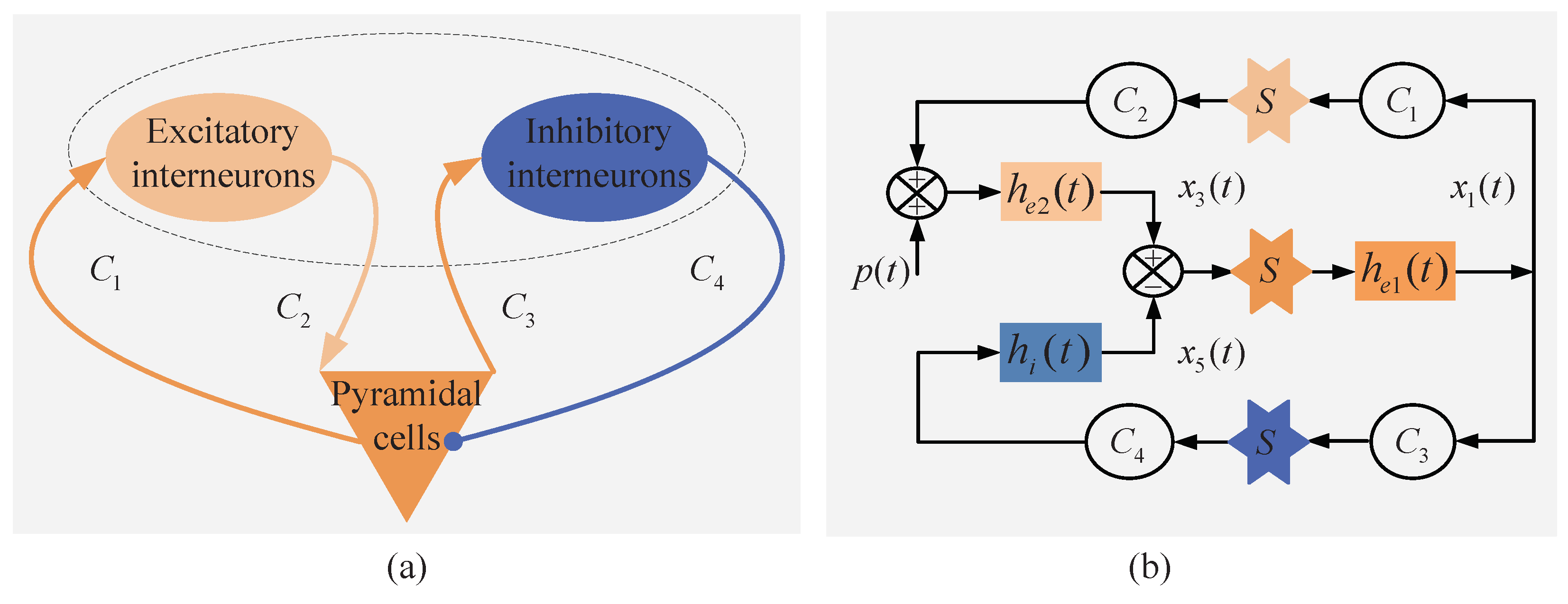
2.2. Neural Mass Model
3. Scheme and Methods
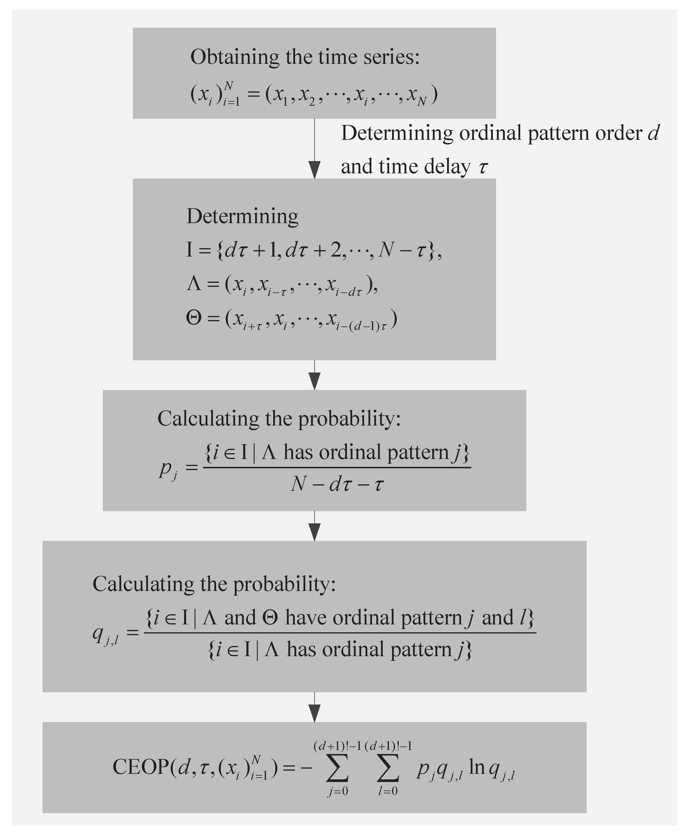
3.1. Conditional Entropy of Ordinal Patterns
3.2. Variation Coefficient
3.3. k-Fold Cross-Validation
3.4. Evaluation Index
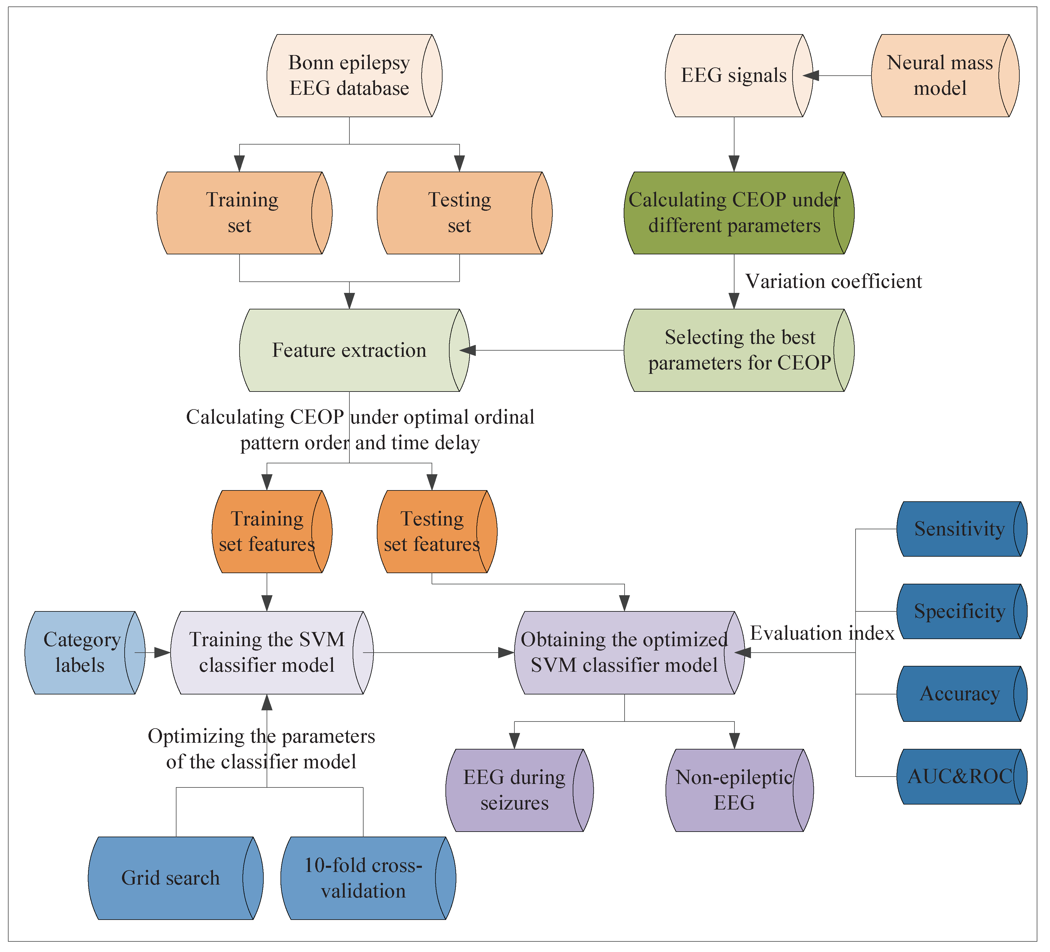
3.5. Overall Scheme
| Algorithm 1: Optimizing the parameters of the Support vector machine (SVM) classifier based on 10-fold cross-validation and grid search. |
 |
4. Results
4.1. Parameters Selection of the CEOP
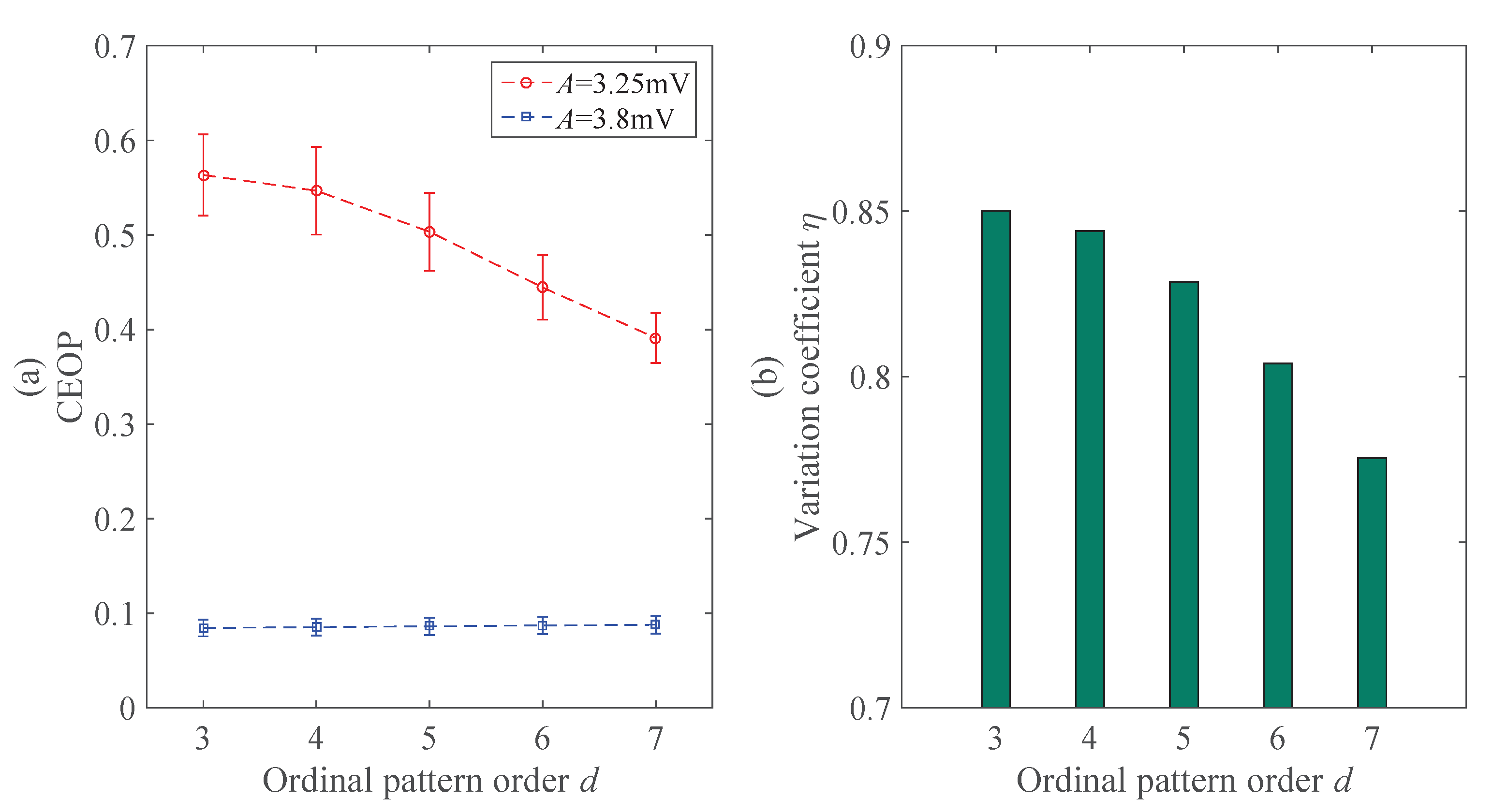
4.1.1. Ordinal Pattern Order d
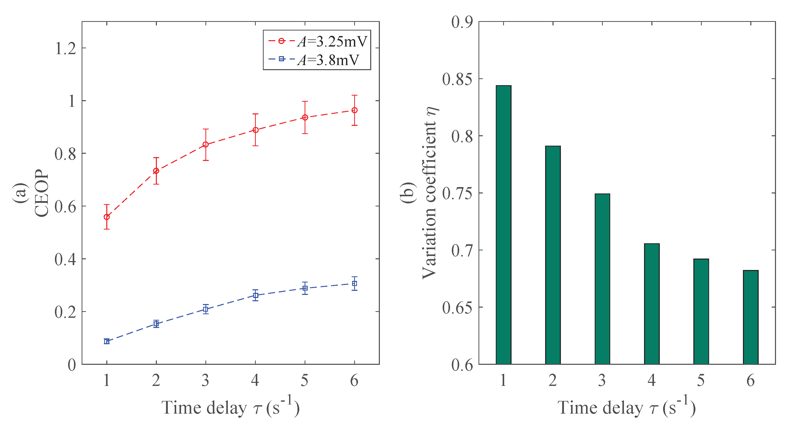
4.1.2. Time Delay
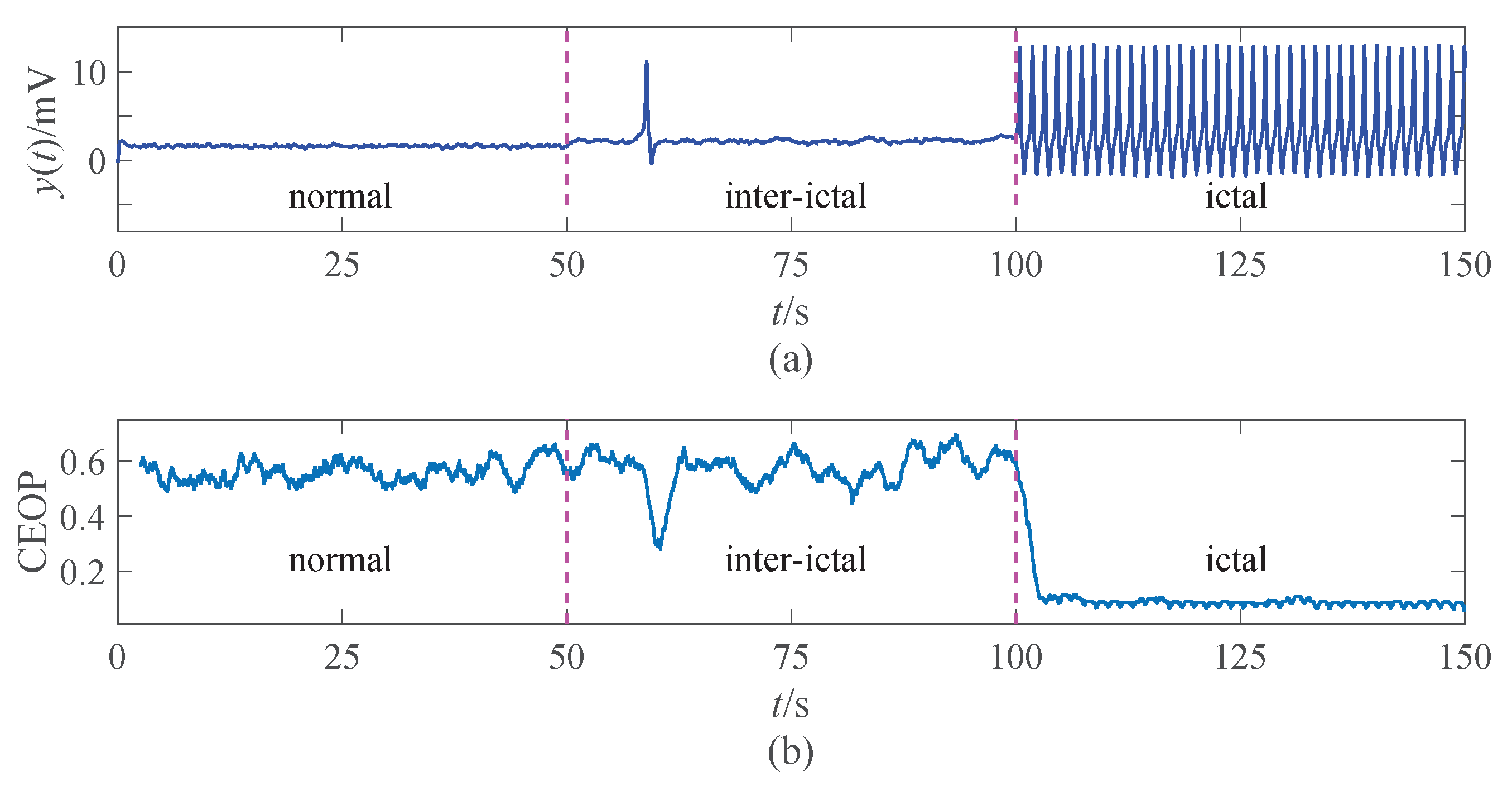
4.2. Performances Analysis of the CEOP
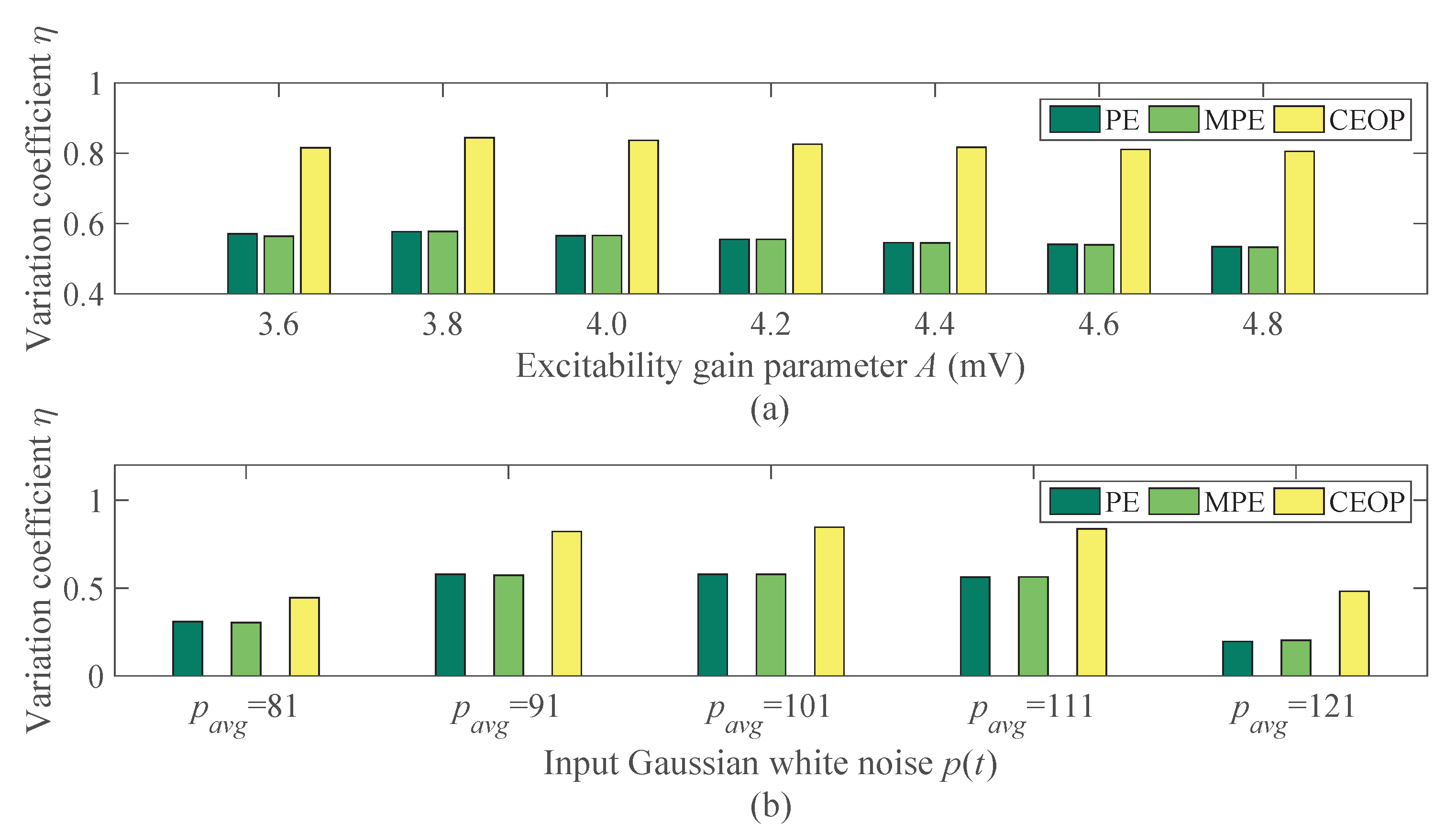
4.2.1. The Analysis Result of Signals under Different Excitability Gain Parameter A
4.2.2. The Analysis Result of Signals under Different Input Gaussian White Noise
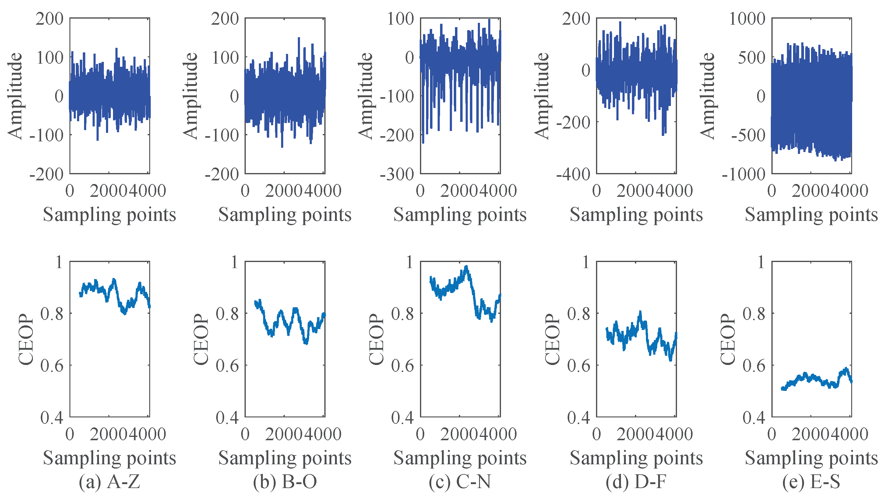
4.3. Experimental Processes and Results
5. Discussions
6. Conclusions
Author Contributions
Funding
Conflicts of Interest
References
- Briggs, F.B.S.; Wilson, B.K.; Pyatka, N.; Colón-Zimmermann, K.; Sajatovic, M.M. Effects of a Remotely Delivered Group-Format Epilepsy Self-Management Program on Adverse Health Outcomes in Vulnerable People with Epilepsy: A Causal Mediation Analysis. Epilepsy Res. 2020, 162, 106303. [Google Scholar] [CrossRef]
- Rodríguez-Cruces, R.; Bernhardt, B.C.; Concha, L. Multidimensional Associations Between Cognition and Connectome Organization in Temporal Lobe Epilepsy. NeuroImage 2020, 213, 116706. [Google Scholar] [CrossRef]
- Budde, R.B.; Arafat, M.A.; Pederson, D.J.; Lovick, T.A.; Jefferys, J.G.R.; Irazoqui, P.P. Acid Reflux Induced Laryngospasm as a Potential Mechanism of Sudden Death in Epilepsy. Epilepsy Res. 2018, 148, 23–31. [Google Scholar] [CrossRef]
- Christiaen, E.; Goossens, M.G.; Descamps, B.; Larsen, L.E.; Boon, P.; Raedt, R.; Vanhove, C. Dynamic Functional Connectivity and Graph Theory Metrics in a Rat Model of Temporal Lobe Epilepsy Reveal a Preference for Brain States with a Lower Functional Connectivity, Segregation and Integration. Neurobiol. Dis. 2020, 139, 104808. [Google Scholar] [CrossRef]
- Jin, Y.; Zhao, C.Z.; Chen, L.H.; Liu, X.Y.; Pan, S.X.; Ju, D.S.; Ma, J.; Li, J.Y.; Wei, B. Identification of Novel Gene and Pathway Targets for Human Epilepsy Treatment. Biol. Res. 2016, 49, 3. [Google Scholar] [CrossRef] [PubMed]
- Kurbatova, P.; Wendling, F.; Kaminska, A.; Rosati, A.; Nabbout, R.; Guerrini, R.; Dulac, O.; Pons, G.; Cornu, C.; Nony, P.; et al. Dynamic Changes of Depolarizing GABA in a Computational Model of Epileptogenic Brain: Insight for Dravet Syndrome. Exp. Neurol. 2016, 283, 57–72. [Google Scholar] [CrossRef] [PubMed]
- Malagarriga, D.; Pons, A.J.; Villa, A.E.P. Complex Temporal Patterns Processing by a Neural Mass Model of a Cortical Column. Cogn. Neurodyn. 2019, 13, 379–392. [Google Scholar] [CrossRef] [PubMed]
- Liu, C.; Zhou, C.S.; Wang, J.; Fietkiewicz, C.; Loparo, K.A. The Role of Coupling Connections in a Model of the Cortico-Basal Ganglia-Thalamocortical Neural Loop for the Generation of Beta Oscillations. Neural Netw. 2020, 123, 381–392. [Google Scholar] [CrossRef]
- Hebbink, J.; van Gils, S.A.; Meijer, H.J.E. On Analysis of Inputs Triggering Large Nonlinear Neural Responses Slow-Fast Dynamics in the Wendling Neural Mass Model. Commun. Nonlinear Sci. Numer. Simul. 2020, 83, 105103. [Google Scholar] [CrossRef]
- Jansen, B.H.; Rit, V.G. Electroencephalogram and Visual Evoked Potential Generation in a Mathematical Model of Coupled Cortical Columns. Biol. Cybern. 1995, 73, 357–366. [Google Scholar] [CrossRef]
- Sharma, M.; Patel, S.; Acharya, U.R. Automated Detection of Abnormal EEG Signals Using Localized Wavelet Filter Banks. Pattern Recognit. Lett. 2020, 133, 188–194. [Google Scholar] [CrossRef]
- Wang, G.J.; Deng, Z.H.; Choi, K.S. Detection of Epilepsy with Electroencephalogram Using Rule-Based Classifiers. Neurocomputing 2017, 228, 283–290. [Google Scholar] [CrossRef]
- Polat, K.; Günes, S. Classification of Epileptiform EEG Using a Hybrid System Based on Decision Tree Classifier and Fast Fourier Transform. Appl. Math. Comput. 2007, 187, 1017–1026. [Google Scholar] [CrossRef]
- Vézard, L.; Legrand, P.; Chavent, M.; Faïta-Aïnseba, F.; Trujillo, L. EEG Classification for the Detection of Mental States. Appl. Soft Comput. 2015, 32, 113–131. [Google Scholar] [CrossRef]
- Yuan, S.S.; Zhou, W.D.; Wu, Q.; Zhang, Y.L. Epileptic Seizure Detection with Log-Euclidean Gaussian Kernel-Based Sparse Representation. Int. J. Neural Syst. 2016, 26, 1650011. [Google Scholar] [CrossRef] [PubMed]
- Seo, J.H.; Tsuda, T.; Lee, Y.J.; Ikeda, A.; Matsuhashi, M.; Matsumoto, R.; Kikuchi, T.; Kang, H. Pattern Recognition in Epileptic EEG Signals via Dynamic Mode Decomposition. Mathematics 2020, 8, 481. [Google Scholar] [CrossRef]
- Fu, K.; Qu, J.F.; Chai, Y.; Zou, T. Hilbert Marginal Spectrum Analysis for Automatic Seizure Detection in EEG Signals. Biomed. Signal Process. Control 2015, 18, 179–185. [Google Scholar] [CrossRef]
- Deriche, M.; Arafat, S.; Al-Insaif, S.; Siddiqui, M. Eigenspace Time Frequency Based Features for Accurate Seizure Detection from EEG Data. IRBM 2019, 40, 122–132. [Google Scholar] [CrossRef]
- Nascimento, D.C.; Depetri, G.; Stefano, L.H.; Anacleto, O.; Leite, J.P.; Edwards, D.J.; Santos, T.E.G.; Neto, F.L. Entropy Analysis of High-Definition Transcranial Electric Stimulation Effects on EEG Dynamics. Brain Sci. 2020, 9, 208. [Google Scholar] [CrossRef]
- Ibáñez-Molina, A.J.; Iglesias-Parro, S.; Escudero, J. Differential Effects of Simulated Cortical Network Lesions on Synchrony and EEG Complexity. Int. J. Neural Syst. 2019, 29, 1850024. [Google Scholar]
- Echegoyen, I.; López-Sanz, D.; Martínez, J.H.; Maestú, F.; Buldú, J.M. Permutation Entropy and Statistical Complexity in Mild Cognitive Impairment and Alzheimer’s Disease: An Analysis Based on Frequency Bands. Entropy 2020, 22, 116. [Google Scholar] [CrossRef]
- Harezlak, K.; Kasprowski, P. Application of Time-Scale Decomposition of Entropy for Eye Movement Analysis. Entropy 2020, 22, 168. [Google Scholar] [CrossRef]
- Hussain, W.; Wang, B.; Niu, Y.; Gao, Y.; Wang, X.; Sun, J.; Zhang, Q.H.; Cao, R.; Zhou, M.N.; Iqbal, M.S.; et al. Epileptic Seizure Detection With Permutation Fuzzy Entropy Using Robust Machine Learning Techniques. IEEE Access 2019, 7, 182238182258. [Google Scholar] [CrossRef]
- Nicolini, C.; Forcellini, G.; Minati, L.; Bifone, A. Scale-Resolved Analysis of Brain Functional Connectivity Networks with Spectral Entropy. NeuroImage 2020, 211, 116603. [Google Scholar] [CrossRef] [PubMed]
- Liu, X.; Wang, G.; Gao, J.; Gao, Q. A Quantitative Analysis for EEG Signals Based on Modified Permutation-Entropy. IRBM 2017, 38, 71–77. [Google Scholar] [CrossRef]
- Liu, X.; Zhao, C.Y.; Sun, C.X.; Chen, Z.M.; Hayat, T.; Alsaedi, A. A New Closed-Loop Strategy for Detection and Modulation of Epileptiform Spikes Based on Cross Approximate Entropy. J. Integr. Neurosci. 2018, 17, 271–280. [Google Scholar]
- Unakafov, A.M.; Keller, K. Conditional Entropy of Ordinal Patterns. Physica D 2014, 269, 94–102. [Google Scholar] [CrossRef]
- Keller, K.; Unakafov, A.M.; Unakafova, V.A. Ordinal Patterns, Entropy, and EEG. Entropy 2014, 16, 6212–6239. [Google Scholar] [CrossRef]
- Unakafov, A.M.; Keller, K. Change-Point Detection Using the Conditional Entropy of Ordinal Patterns. Entropy 2018, 20, 709. [Google Scholar] [CrossRef]
- Mougoufan, J.B.B.à.; Fouda, J.S.A.E.; Tchuente, M.; Koepf, W. Adaptive ECG Beat Classification by Ordinal Pattern Based Entropies. Commun. Nonlinear Sci. Numer. Simul. 2020, 84, 105156. [Google Scholar] [CrossRef]
- Rubega, M.; Scarpa, F.; Teodori, D.; Sejling, A.S.; Frandsen, C.S.; Sparacino, G. Detection of Hypoglycemia Using Measures of EEG Complexity in Type 1 Diabetes Patients. Entropy 2020, 22, 81. [Google Scholar] [CrossRef]
- Wendling, F.; Bellanger, J.J.; Bartolomei, F.; Chauvel, P. Relevance of Nonlinear Lumped-parameter Models in the Analysis of Depth-EEG Epileptic Signals. Biol. Cybern. 2000, 83, 367–378. [Google Scholar] [CrossRef] [PubMed]
- Lopes da Silva, F.H.; Blanes, W.; Kalitzin, S.N.; Parra, J.; Suffczynski, P.; Velis, D.N. Dynamical Diseases of Brain Systems: Different Routes to Epileptic Seizures. IEEE. Trans. Biomed. Eng. 2003, 50, 540–548. [Google Scholar] [CrossRef] [PubMed]
- Unakafova, V.A.; Keller, K. Efficiently Measuring Complexity on the Basis of Real-World Data. Entropy 2013, 15, 4392–4415. [Google Scholar] [CrossRef]
- Riedl, M.; Müller, A.; Wessel, N. Practical Considerations of Permutation Entropy. Eur. Phys. J. Spec. Top. 2013, 222, 249–262. [Google Scholar] [CrossRef]
- Nicolaou, N.; Georgiou, J. Detection of Epileptic Electroencephalogram Based on Permutation Entropy and Support Vector Machines. Expert Syst. Appl 2012, 39, 202–209. [Google Scholar] [CrossRef]
- Burges, C.J. A Tutorial on Support Vector Machines for Pattern Recognition. Data Min. Knowl. Discov. 1998, 2, 121–167. [Google Scholar] [CrossRef]
- Keerthi, S.S.; Lin, C.J. Asymptotic Behaviors of Support Vector Machines with Gaussian Kernel. Neural Comput. 2003, 15, 1667–1689. [Google Scholar] [CrossRef]
- Wendling, F.; Bartolomei, F.; Bellanger, J.J.; Chauvel, P. Epileptic Fast Activity Can Be Explained by a Model of Impaired GABAergic Dendritic Inhibition. Eur. J. Neurosci. 2002, 15, 1499–1508. [Google Scholar] [CrossRef]
- Andrzejak, R.G.; Lehnertz, K.; Mormann, F.; Rieke, C.; David, P.; Elger, C.E. Indications of Nonlinear Deterministic and Finite Dimensional Structures in Time Series of Brain Electrical Activity: Dependence on Recording Region and Brain State. Phys. Rev. E 2001, 64, 061907. [Google Scholar] [CrossRef] [PubMed]
- Iscan, Z.; Dokur, Z.; Demiralp, T. Classification of Electroencephalogram Signals with Combined Time and Frequency Features. Expert Syst. Appl. 2011, 38, 10499–10505. [Google Scholar] [CrossRef]
- Swami, P.; Gandhi, T.K.; Panigrahi, B.K.; Tripathi, M.; Anand, S. A Novel Robust Diagnostic Model to Detect Seizures in Electroencephalography. Expert Syst. Appl. 2016, 56, 116–130. [Google Scholar] [CrossRef]
- Zhou, D.M.; Li, X.M. Epilepsy EEG Signal Classification Algorithm Based on Improved RBF. Front. Neurosci. 2020, 14, 606. [Google Scholar] [CrossRef] [PubMed]
- Qiu, Y.; Zhou, W.D.; Yu, N.N.; Du, P.D. Denoising Sparse Autoencoder-Based Ictal EEG Classification. IEEE Trans. Neural Syst. Rehabil. Eng. 2018, 26, 1717–1726. [Google Scholar] [CrossRef]
- Jiang, Y.; Chen, W.Z.; Zhang, T.; Li, M.Y.; You, Y.; Zheng, X. Developing Multi-Component Dictionary-Based Sparse Representation for Automatic Detection of Epileptic EEG Spikes. Biomed. Signal Process. Control 2020, 60, 101966. [Google Scholar] [CrossRef]
- Kannathal, N.; Choo, M.L.; Acharya, U.R.; Sadasivan, P.K. Entropies for Detection of Epilepsy in EEG. Comput. Methods Programs Biomed. 2005, 80, 187–194. [Google Scholar] [CrossRef]
- Subasi, A. EEG Signal Classification Using Wavelet Feature Extraction and A Mixture of Expert Model. Expert Syst. Appl. 2007, 32, 1084–1093. [Google Scholar] [CrossRef]


| Data Sets | A-Z | B-O | C-N | D-F | E-S | |
|---|---|---|---|---|---|---|
| Category | ||||||
| Experimental subject | Five healthy volunteers | Five epilepsy patients | ||||
| EEG type | Scalp | Scalp | Intracranial | Intracranial | Intracranial | |
| EEG | EEG | EEG | EEG | EEG | ||
| Subject status | Awake, | Awake, | Inter-ictal | Inter-ictal | Ictal | |
| eyes open | eyes closed | stage | stage | stage | ||
| Electrode placement | International | International | Hippocampus | Within | Within | |
| 10-20 | 10-20 | opposite to | epileptogenic | epileptogenic | ||
| system | system | hemisphere | zone | zone | ||
| Number of subsets | 100 | 100 | 100 | 100 | 100 | |
| Sampling points | 4097 | 4097 | 4097 | 4097 | 4097 | |
| Sampling frequency | 173.61Hz | 173.61Hz | 173.61Hz | 173.61Hz | 173.61Hz | |
| Category | True Value | Predicted Value |
|---|---|---|
| TP | positive | positive |
| FP | negative | positive |
| TN | negative | negative |
| FN | positive | negative |
| Category | A (mV) | Mean | Std | ||||
|---|---|---|---|---|---|---|---|
| PE | MPE | CEOP | PE | MPE | CEOP | ||
| Normal | 3.25 | 0.6124 | 0.6164 | 0.5590 | 0.0319 | 0.0230 | 0.0468 |
| 3.6 | 0.2628 | 0.2686 | 0.1031 | 0.0302 | 0.0133 | 0.0205 | |
| 3.8 | 0.2590 | 0.2604 | 0.0872 | 0.0135 | 0.0111 | 0.0098 | |
| 4.0 | 0.2660 | 0.2675 | 0.0913 | 0.0064 | 0.0053 | 0.0062 | |
| Seizure | 4.2 | 0.2722 | 0.2741 | 0.0973 | 0.0132 | 0.0102 | 0.0093 |
| 4.4 | 0.2780 | 0.2804 | 0.1021 | 0.0164 | 0.0083 | 0.0114 | |
| 4.6 | 0.2810 | 0.2836 | 0.1055 | 0.0172 | 0.0042 | 0.0120 | |
| 4.8 | 0.2851 | 0.2879 | 0.1087 | 0.0167 | 0.0021 | 0.0120 | |
| Category | Mean | Std | |||||
|---|---|---|---|---|---|---|---|
| PE | MPE | CEOP | PE | MPE | CEOP | ||
| 81 | 0.6143 | 0.6184 | 0.5600 | 0.0336 | 0.0234 | 0.0510 | |
| 91 | 0.6109 | 0.6150 | 0.5572 | 0.0297 | 0.0207 | 0.0432 | |
| Normal (A= 3.25 mV) | 101 | 0.6089 | 0.6128 | 0.5572 | 0.0327 | 0.0224 | 0.0508 |
| 111 | 0.6142 | 0.6187 | 0.5636 | 0.0356 | 0.0207 | 0.0514 | |
| 121 | 0.3455 | 0.3505 | 0.1877 | 0.0396 | 0.0281 | 0.0468 | |
| 81 | 0.4245 | 0.4301 | 0.3109 | 0.0565 | 0.0361 | 0.0705 | |
| 91 | 0.2578 | 0.2626 | 0.0994 | 0.0305 | 0.0129 | 0.0200 | |
| Seizure (A= 3.8 mV) | 101 | 0.2569 | 0.2585 | 0.0857 | 0.0146 | 0.0116 | 0.0102 |
| 111 | 0.2690 | 0.2703 | 0.0916 | 0.0053 | 0.0042 | 0.0052 | |
| 121 | 0.2777 | 0.2793 | 0.0973 | 0.0120 | 0.0095 | 0.0088 | |
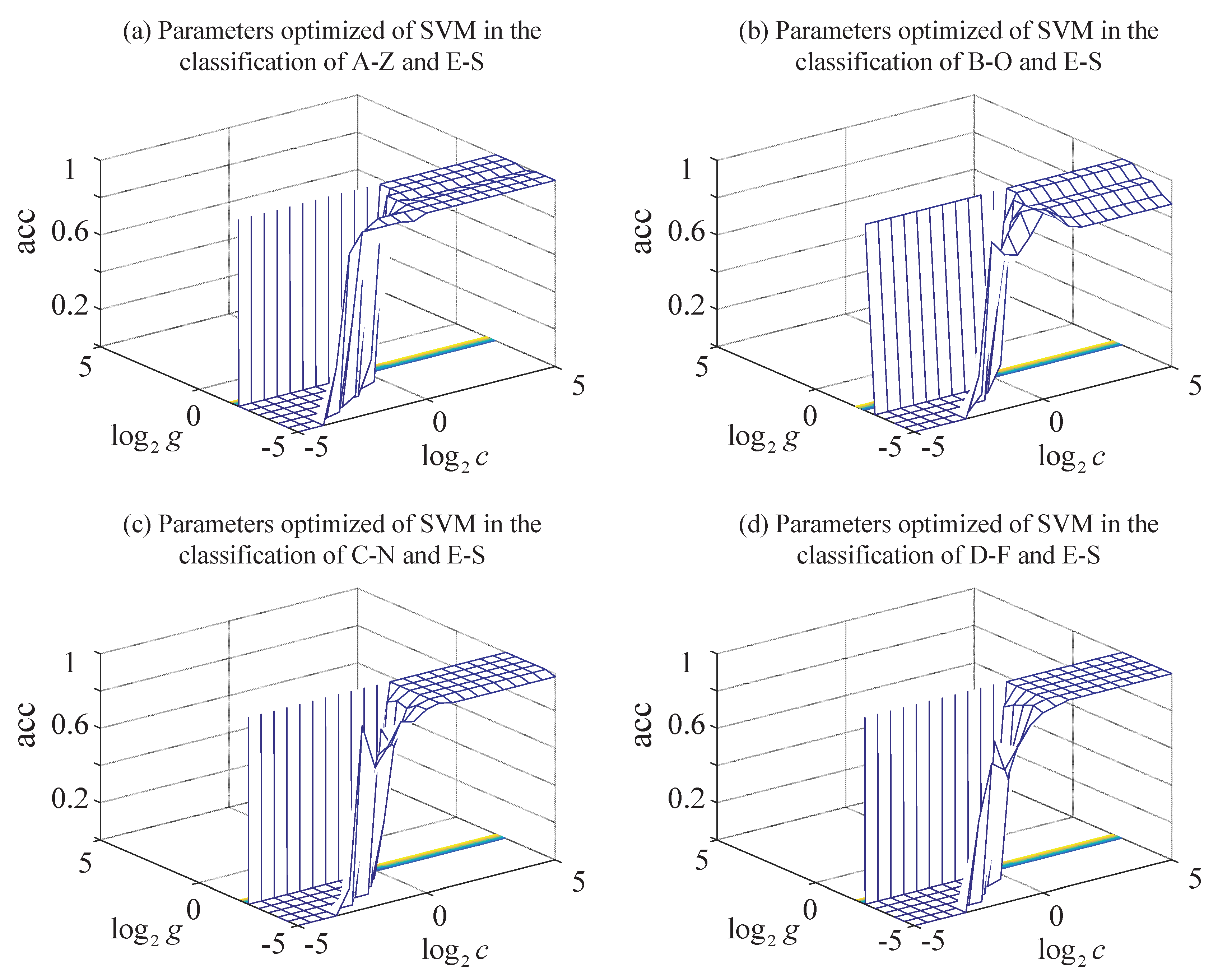
| Classification | A-Z, E-S | B-O, E-S | C-N, E-S | D-F, E-S | |
|---|---|---|---|---|---|
| Category | |||||
| 1 | 1 | 1.4142 | 2 | ||
| 0.0313 | 0.0313 | 0.0313 | 0.0313 | ||
| (%) | 96.25 | 81.25 | 90.63 | 88.75 | |
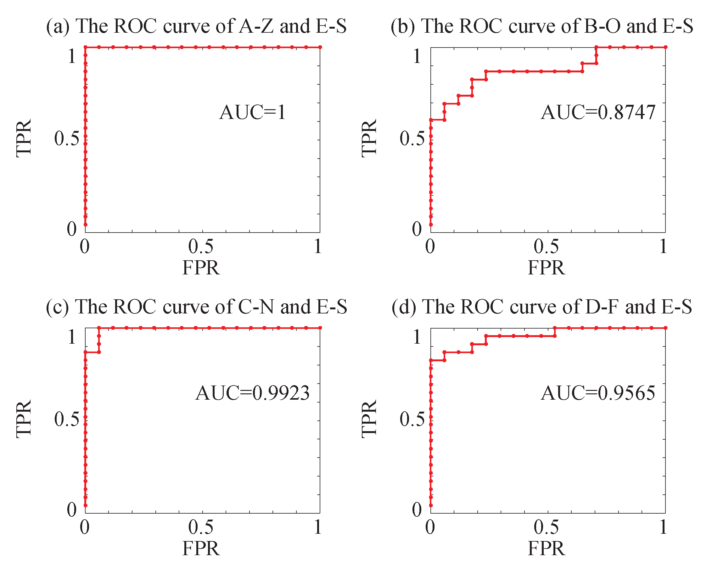
| Classification | A-Z, E-S | B-O, E-S | C-N, E-S | D-F, E-S | |
|---|---|---|---|---|---|
| Evaluation Index | |||||
| Sensitivity (%) | 100 | 80.00 | 88.46 | 86.96 | |
| Specificity (%) | 89.47 | 80.00 | 100 | 82.35 | |
| Accuracy (%) | 95.00 | 80.00 | 92.50 | 85.00 | |
| AUC | 1 | 0.8747 | 0.9923 | 0.9565 | |
| Authors | Method (Features Extraction & Classifier) | Number of Extracted Features | Accuracy (%) |
|---|---|---|---|
| Kannathal et al. [46] | Entropy measures & | 4 | 92.22 |
| (2005) | Adaptive neuro-fuzzy inference system (ANFIS) | ||
| Subasi [47] | Discrete wavelet transform (DWT) & | 16 | 94.50 |
| (2007) | Mixture of experts (ME) | ||
| Iscan et al. [41] | Cross correlation (CC), power spectral density (PSD) & | 2 | 100 |
| (2011) | Least squares support vector machine (LS-SVM) | ||
| Nicolaou et al. [36] | Permutation entropy (PE) & | 1 | 93.55 |
| (2012) | Support vector machine (SVM) | ||
| Fu et al. [17] | Hilbert marginal spectrum analysis (HMS) & | 8 | 99.85 |
| (2015) | Support vector machine (SVM) | ||
| Swami et al. [42] | Dual-tree complex wavelet transform (DTCWT) & | 6 | 100 |
| (2016) | General regression neural network (GRNN) | ||
| Deriche et al. [18] | Singular value decomposition (SVD) & | 2 | 99.30 |
| (2019) | Multilayer perceptron network (MLP) | ||
| Zhou et al. [43] | Wave coefficients, entropy measures & | 4 | 96.30 |
| (2020) | Improved convolution neural network (CNN) | ||
| This work | Conditional entropy of ordinal patterns (CEOP) & | 1 | 95.00 |
| Support vector machine (SVM) |
© 2020 by the authors. Licensee MDPI, Basel, Switzerland. This article is an open access article distributed under the terms and conditions of the Creative Commons Attribution (CC BY) license (http://creativecommons.org/licenses/by/4.0/).
Share and Cite
Liu, X.; Fu, Z. A Novel Recognition Strategy for Epilepsy EEG Signals Based on Conditional Entropy of Ordinal Patterns. Entropy 2020, 22, 1092. https://doi.org/10.3390/e22101092
Liu X, Fu Z. A Novel Recognition Strategy for Epilepsy EEG Signals Based on Conditional Entropy of Ordinal Patterns. Entropy. 2020; 22(10):1092. https://doi.org/10.3390/e22101092
Chicago/Turabian StyleLiu, Xian, and Zhuang Fu. 2020. "A Novel Recognition Strategy for Epilepsy EEG Signals Based on Conditional Entropy of Ordinal Patterns" Entropy 22, no. 10: 1092. https://doi.org/10.3390/e22101092
APA StyleLiu, X., & Fu, Z. (2020). A Novel Recognition Strategy for Epilepsy EEG Signals Based on Conditional Entropy of Ordinal Patterns. Entropy, 22(10), 1092. https://doi.org/10.3390/e22101092