Uncertainty Quantification of Film Cooling Performance of an Industrial Gas Turbine Vane

 ,
,
Abstract
1. Introduction
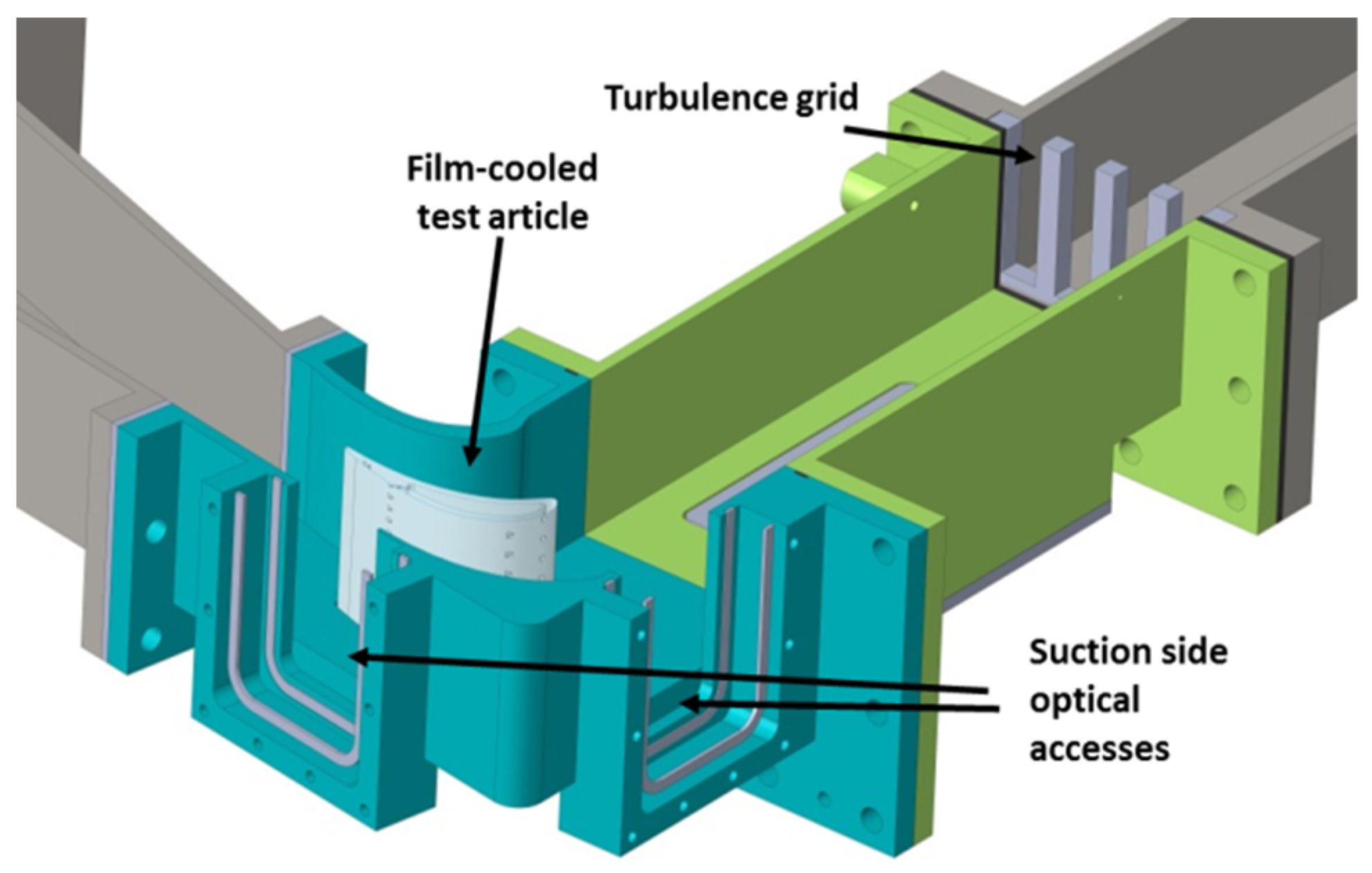
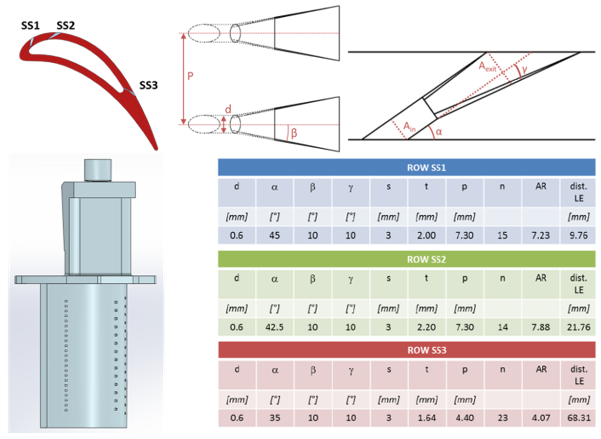
2. Test Case
3. Numerical Methodology
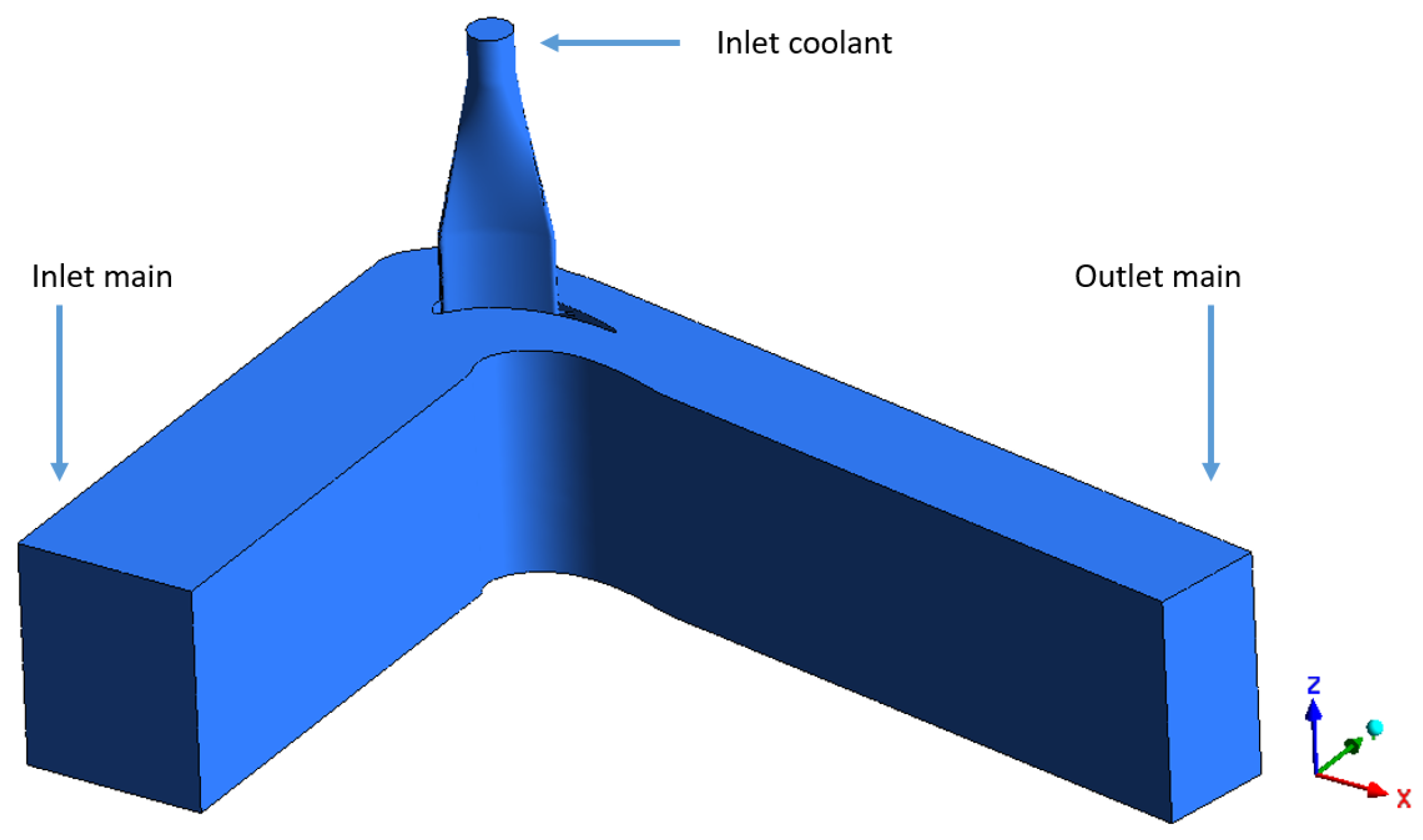
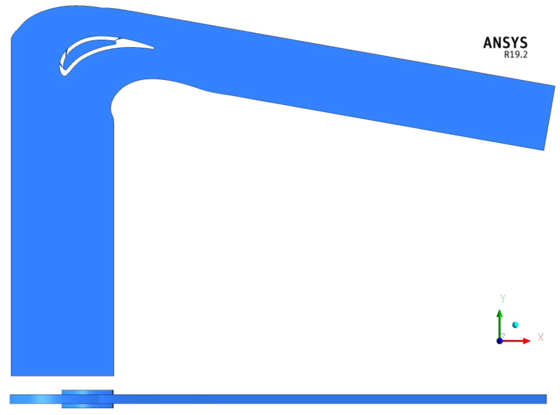
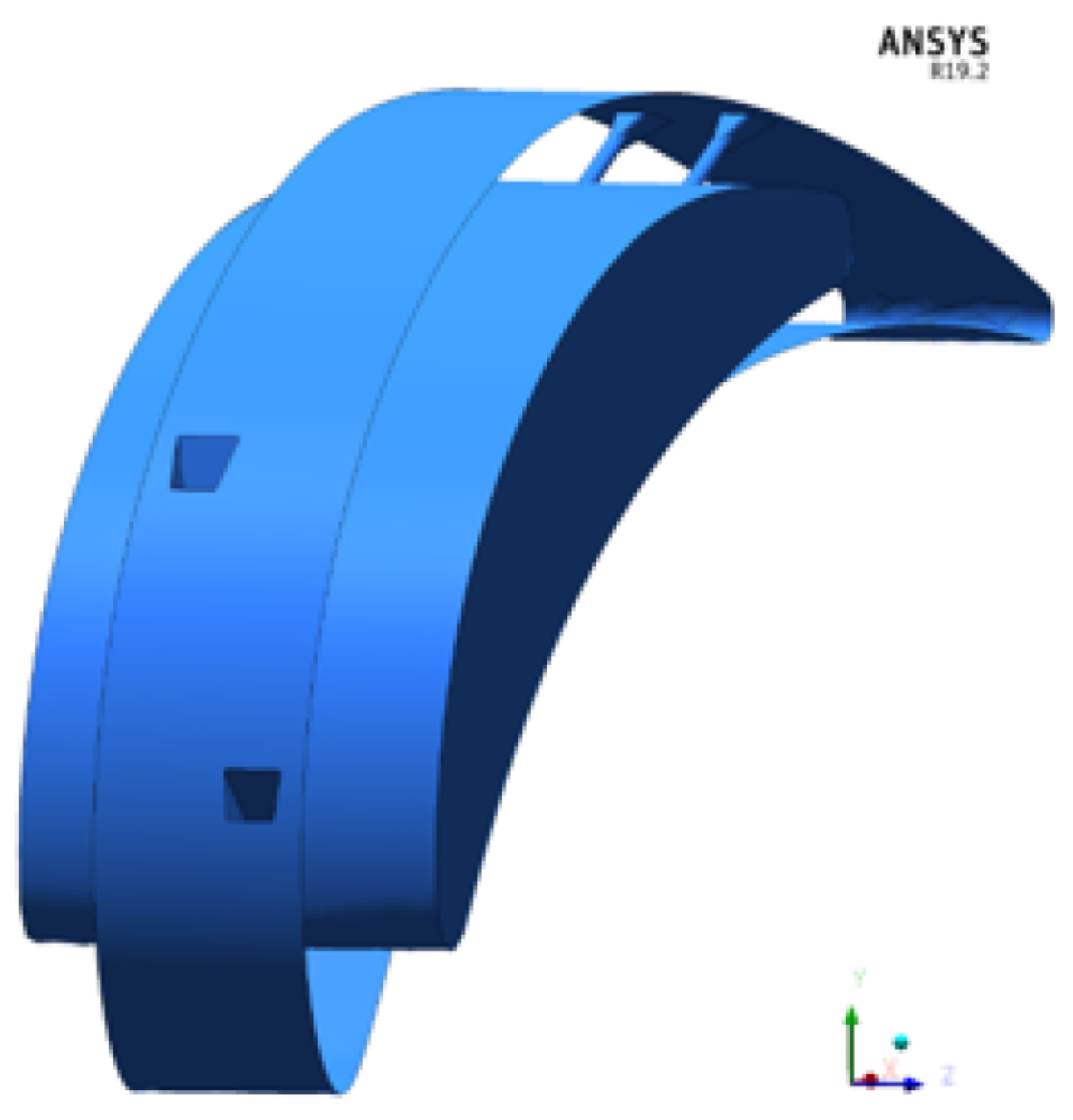
3.1. Geometry
3.2. Numerical Setup
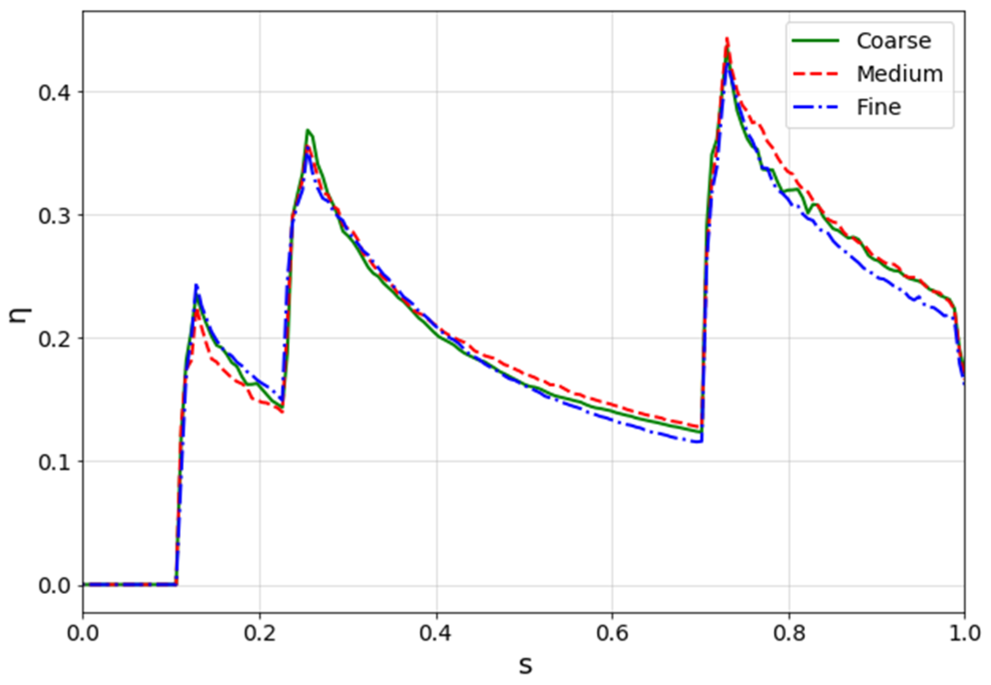
3.3. Mesh Sensitivity
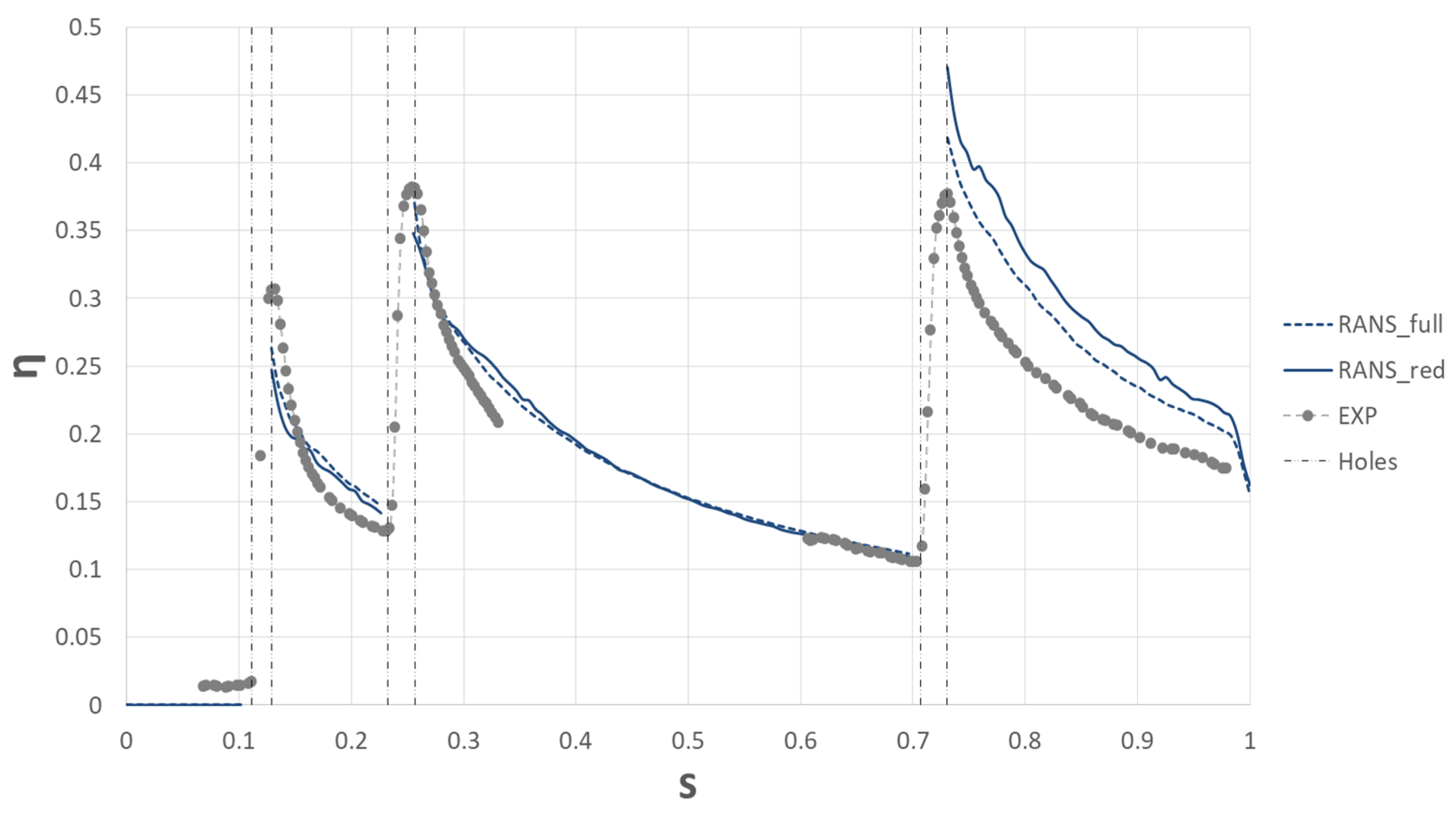
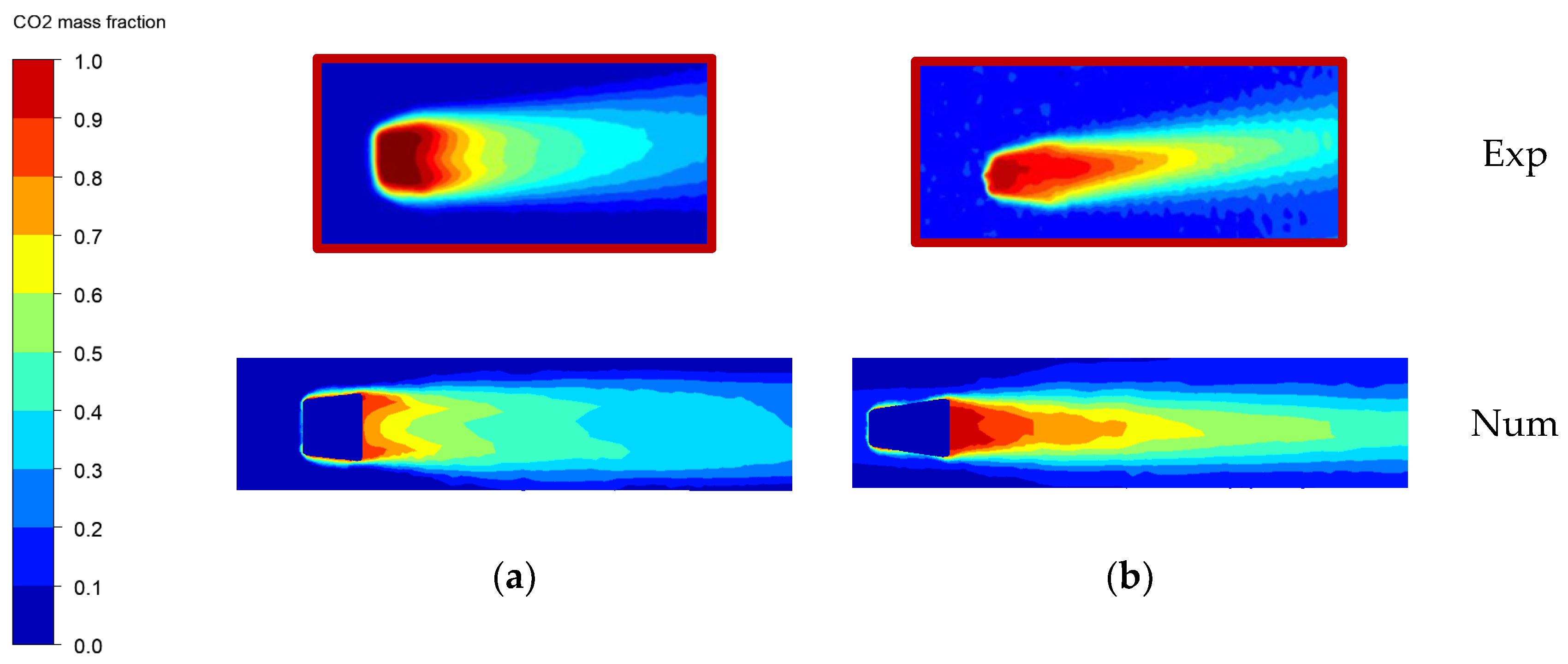
3.4. Results
3.5. Unsteady Approach
4. Uncertainty Quantification
4.1. Methodology
4.2. Input Uncertainties
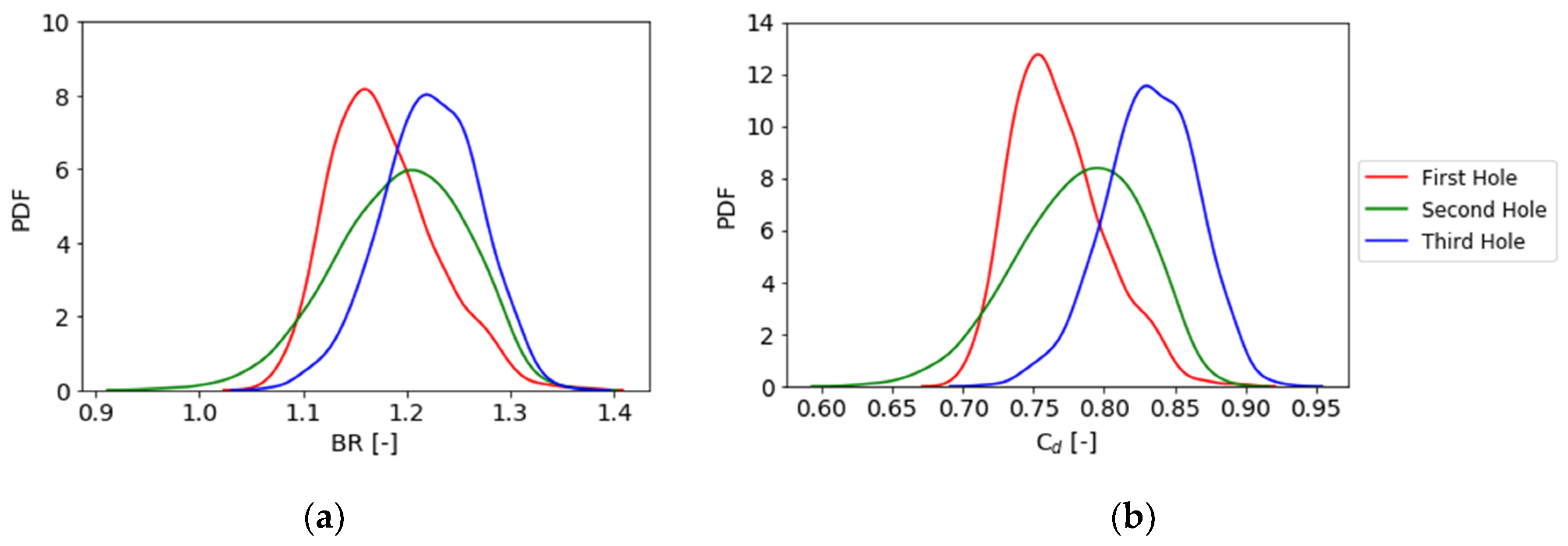
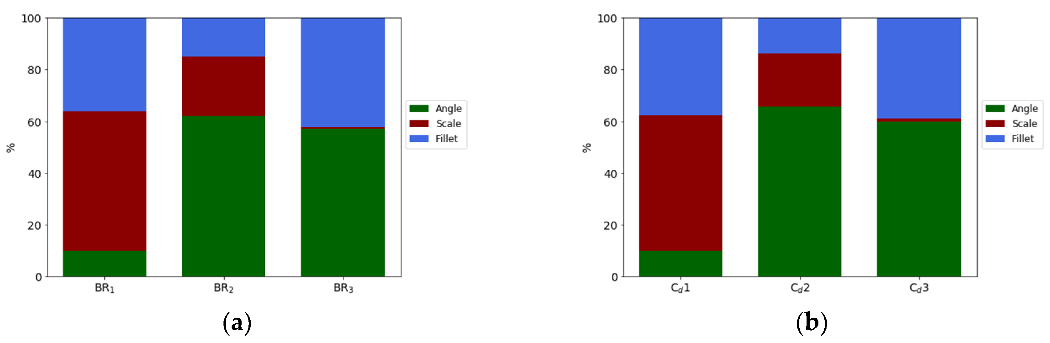
4.3. Results
5. Conclusions
Author Contributions
Funding
Acknowledgments
Conflicts of Interest
References
- Bacci, T.; Gamannossi, A.; Mazzei, L.; Picchi, A.; Winchler, L.; Carcasci, C.; Andreini, A.; Abba, L.; Vagnoli, S. Experimental and CFD analyses of a high-loaded gas turbine blade. Energy Procedia 2017, 126, 770–777. [Google Scholar] [CrossRef]
- Bacci, T.; Picchi, A.; Facchini, B. Flat Plate and Turbine Vane Film-Cooling Performance with Laid-Back Fan-Shaped Holes. Int. J. Turbomach. Propuls. Power 2019, 4, 14. [Google Scholar] [CrossRef]
- Bohn, D.; Ren, J.; Kusterer, K. Conjugate Heat Transfer Analysis for Film Cooling Configurations. With Different Hole Geometries. In Proceedings of the ASME Turbo Expo–GT2003-38369, Atlanta, GA, USA, 1 January 2003. [Google Scholar]
- Bogard, D.; Thole, K. Gas turbine film cooling. ASME J. Propuls. Power 2006, 2, 249–270. [Google Scholar] [CrossRef]
- Du, H.; Mei, Z.; Zou, J.; Jiang, W.; Xie, D. Conjugate Heat Transfer Investigation on Swirl-Film Cooling at the Leading Edge of a Gas Turbine Vane. Entropy 2019, 21, 1007. [Google Scholar] [CrossRef]
- Aminossadati, S.M.; Mee, D.J. Uncertainty Analysis for the Measurements of Aerodynamic Loss of Cooled Turbine Blades. In Proceedings of the Fifth Biennial Engineering Mathematics and Applications Conference, Brisbane, Australia, 29 September–2 October 2002. [Google Scholar]
- Farmer, J.; Merino, Z.; Gray, A.; Jacobs, D. Universal Sample Size Invariant Measures for Uncertainty Quantification in Density Estimation. Entropy 2019, 21, 1120. [Google Scholar] [CrossRef]
- Montomoli, F.; D’Ammaro, A.; Uchida, S. Uncertainty Quantification and Conjugate Heat Transfer: A Stochastic Analysis. ASME J. Turbomach. 2013, 135, 031014. [Google Scholar] [CrossRef]
- Le Maître, O.; Knio, O. Spectral Methods for Uncertainty Quantification; Springer: Amsterdam, The Netherlands, 2010. [Google Scholar]
- Wiener, N. The Homogeneous Chaos. Am. J. Math. 1938, 60, 897–936. [Google Scholar] [CrossRef]
- Askey, R.; Wilson, J. Some Basic Hypergeometric Polynomials that Generalized Jacobi Polynomials; American Mathematical Society: Providence, RI, USA, 1985. [Google Scholar]
- Karniadakis, G.; Xiu, D.; Su, C.H.; Lucor, D. Generalized Polynomial Chaos Solution for Differential Equations with Random Inputs; Research report; Seminar für Angewandte Mathematik: Zurich, Switzerland, 2005. [Google Scholar]
- Vaezi, M.; Seitz, H.; Yang, S. A review on 3D micro-additive manufacturing technologies. Int. J. Adv. Manuf. Technol. 2013, 67, 1721–1754. [Google Scholar] [CrossRef]
- Kamath, C. Data mining and statistical inference in selective laser melting. Int. J. Adv. Manuf. Technol. 2016, 86, 1659–1677. [Google Scholar] [CrossRef]
- Lopez, F.; Witherell, P.; Lane, B. Identifying uncertainty in laser powder bed fusion additive manufacturing models. J. Mech. Des. 2016, 138, 114502. [Google Scholar] [CrossRef]
- Shi, W.; Chen, P.; Li, X.; Ren, J.; Jiang, H. Uncertainty Quantification of the Effects of Small Manufacturing Deviations on Film Cooling: A Fan-Shaped Hole. Aerospace 2019, 6, 46. [Google Scholar] [CrossRef]
- Caciolli, G.; Facchini, B.; Picchi, A.; Tarchi, L. Comparison between PSP and TLC steady state techniques for adiabatic effectiveness measurement on a multiperforated plate. Exp. Therm. Fluid Sci. 2013, 48, 122–133. [Google Scholar] [CrossRef]
- Frank, T.; Menter, F. Validation of URANS SST and SBES in ANSYS CFD for the Turbulent Mixing of Two Parallel Planar Water Jets Impinging on a Stationary Pool. In Proceedings of the ASME 2017 Verification and Validation Symposium, Las Vegas, NV, USA, 3–5 May 2017. [Google Scholar]
- Lenzi, T.; Palanti, L.; Picchi, A.; Bacci, T.; Mazzei, L.; Andreini, A.; Facchini, B.; Vitale, I. Time-Resolved Flow Field Analysis of Effusion Cooling System with Representative Swirling Main Flow. In Proceedings of the ASME TURBO EXPO 2019: Power for Land, Sea and Air, Phoenix, AZ, USA, 17–21 June 2019. [Google Scholar]
- Smagorinsky, J. General Circulation Experiments with the Primitive Equations. Mon. Weather Rev. 1963, 91, 99–164. [Google Scholar] [CrossRef]
- Germano, M.; Piomelli, U.; Moin, P.; Cabot, W.H. A Dynamic Subgrid-Scale Eddy Viscosity Model. Phys. Fluids 1991, 3, 1760–1765. [Google Scholar] [CrossRef]
- Germano, M. Turbulence: The Filtering Approach. J. Fluid Mech. 1992, 238, 325–336. [Google Scholar] [CrossRef]
- Adams, B.; Bauman, L.; Bohnhoff, W.; Dalbey, K.; Ebeida, M.; Eddy, J.; Eldred, M.; Hough, P.; Hu, K.; Jakeman, J.; et al. DAKOTA, A Multilevel Parallel Object-Oriented Framework for Design Optimization, Parameter Estimation, Uncertainty Quantification, and Sensitivity Analysis: Version 6.9 User’s Manual 2009. Available online: https://pdfs.semanticscholar.org/5e30/66fd427b1ba4b2a743cc3e042a0dfe9a87f2.pdf (accessed on 29 November 2019).
- Bunker, R. The effects of manufacturing tolerances on gas turbine cooling. In Proceedings of the ASME Turbo Expo 2008: Power for Land, Sea, and Air, Berlin, Germany, 9–13 June 2008. [Google Scholar]
- Montomoli, F.; Massini, M.; Salvadori, S.; Martelli, F. Geometrical Uncertainty and Film Cooling: Fillet Radii. J. Turbomach. 2012, 134, 011019. [Google Scholar] [CrossRef]


| Inlet Mainflow | P0 = 135,770 Pa | T0 = 286.15 K |
| Outlet Mainflow | P0 = 123,279 Pa | |
| Inlet Coolant | P0 = 144,760 Pa | T0 = 286.15 K |
| Coarse | Medium | Fine | |
|---|---|---|---|
| N° Elem | 2.06 M | 3.18 M | 4.33 M |
| N° Nodes | 635 k | 972 k | 1.33 M |
| Angle | Scale | Fillet Radius | |
|---|---|---|---|
| 1 | −2.2° | 0.956 | 2.7% |
| 2 | 2.2° | 0.956 | 2.7% |
| 3 | −2.2° | 1.044 | 2.7% |
| 4 | 2.2° | 1.044 | 2.7% |
| 5 | −2.2° | 0.956 | 7.3% |
| 6 | 2.2° | 0.956 | 7.3% |
| 7 | −2.2° | 1.044 | 7.3% |
| 8 | 2.2° | 1.044 | 7.3% |
© 2019 by the authors. Licensee MDPI, Basel, Switzerland. This article is an open access article distributed under the terms and conditions of the Creative Commons Attribution (CC BY) license (http://creativecommons.org/licenses/by/4.0/).
Share and Cite
Gamannossi, A.; Amerini, A.; Mazzei, L.; Bacci, T.; Poggiali, M.; Andreini, A. Uncertainty Quantification of Film Cooling Performance of an Industrial Gas Turbine Vane. Entropy 2020, 22, 16. https://doi.org/10.3390/e22010016
Gamannossi A, Amerini A, Mazzei L, Bacci T, Poggiali M, Andreini A. Uncertainty Quantification of Film Cooling Performance of an Industrial Gas Turbine Vane. Entropy. 2020; 22(1):16. https://doi.org/10.3390/e22010016
Chicago/Turabian StyleGamannossi, Andrea, Alberto Amerini, Lorenzo Mazzei, Tommaso Bacci, Matteo Poggiali, and Antonio Andreini. 2020. "Uncertainty Quantification of Film Cooling Performance of an Industrial Gas Turbine Vane" Entropy 22, no. 1: 16. https://doi.org/10.3390/e22010016
APA StyleGamannossi, A., Amerini, A., Mazzei, L., Bacci, T., Poggiali, M., & Andreini, A. (2020). Uncertainty Quantification of Film Cooling Performance of an Industrial Gas Turbine Vane. Entropy, 22(1), 16. https://doi.org/10.3390/e22010016