Low-Complexity Rate-Distortion Optimization of Sampling Rate and Bit-Depth for Compressed Sensing of Images

Abstract
1. Introduction
2. Problem Formulation
3. Bit-Rate Model
3.1. Estimation of Information Entropy
3.2. Simplified Model of Average Codeword Length
4. Relative PSNR Model
4.1. Relative PSNR
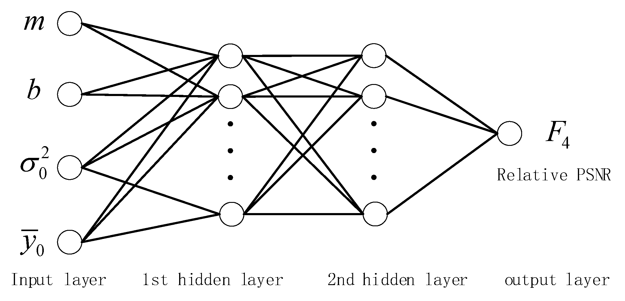
4.2. Relative PSNR Model with Feedforward Neural Network Learning
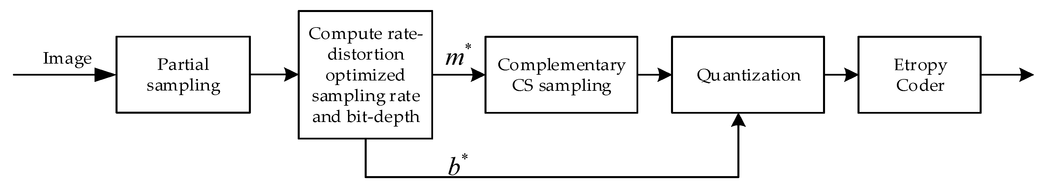
5. Rate-Distortion Optimization for Sampling Rate and Bit-Depth
5.1. Rate-Distortion Optimization Algorithm
- (1)
- Input:
- (2)
- First sampling.
- (3)
- Extracting features.
- (4)
- Reducing the candidate set.
- (5)
- Estimating the optimal parameters.
- (6)
- Second sampling.
- (7)
- Quantization and entropy coding.
5.2. Model Parameter Estimation for the Bit-Rate Model and the Relative PSNR Model
5.3. Computational Complexity of the Rate-Distortion Optimization Algorithm
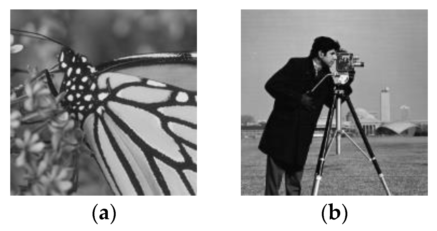
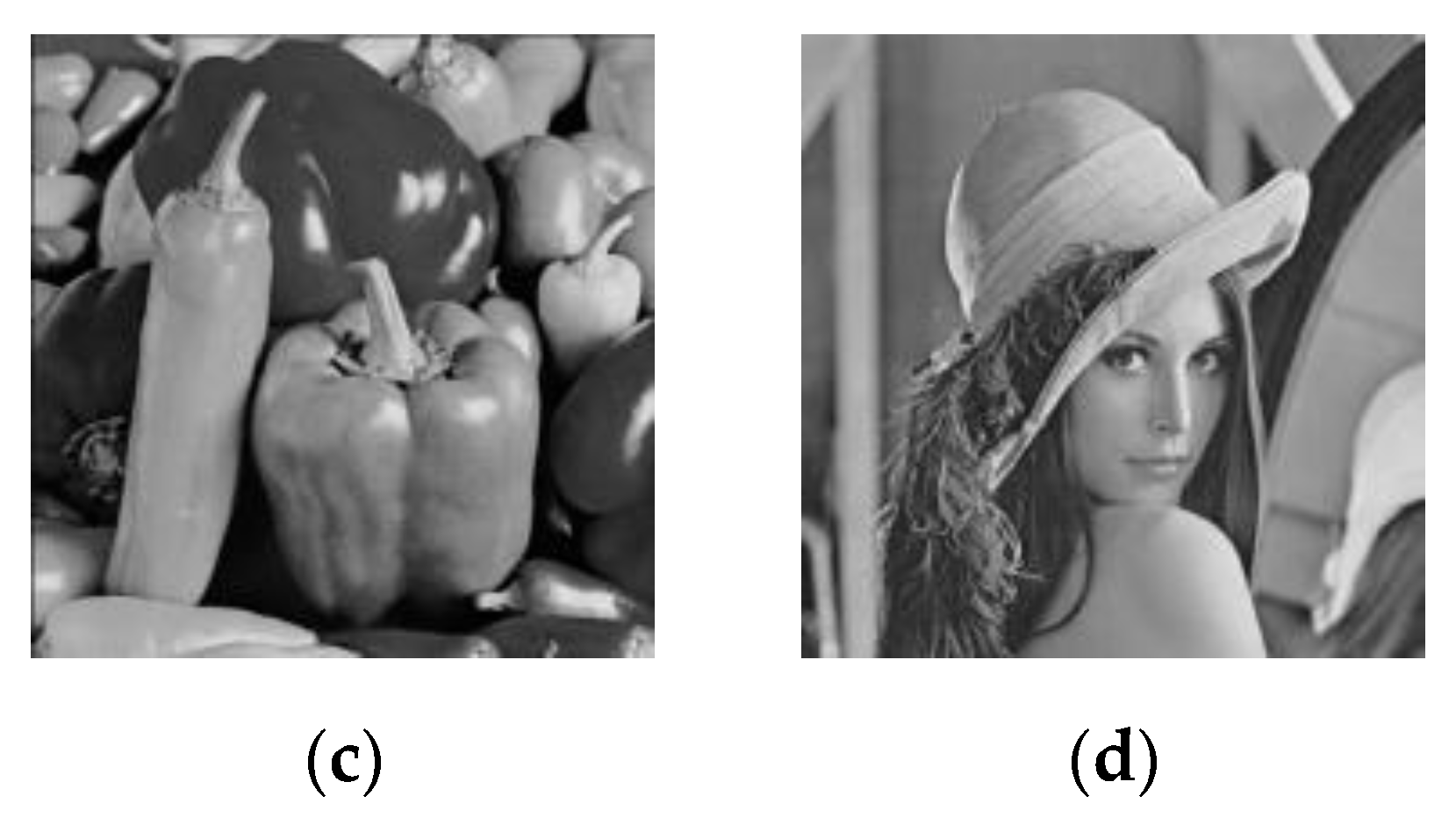
6. Numerical Results and Analysis
7. Conclusions
Author Contributions
Funding
Acknowledgments
Conflicts of Interest
Appendix A
References
- Candès, E.J.; Romberg, J.; Tao, T. Robust Uncertainty Principlesr : Exact Signal Frequency Information. IEEE Trans. Inf. Theory 2006, 52, 489–509. [Google Scholar] [CrossRef]
- Donoho, D.L. Compressed Sensing. IEEE Trans. Inf. Theory 2006, 52, 1289–1306. [Google Scholar] [CrossRef]
- Candès, E.J. Compressive sampling. Proc. Int. Congress Math. Madr. 2006, 3, 1433–1452. [Google Scholar]
- Candès, E.J.; Romberg, J.K.; Tao, T. Stable signal recovery from incomplete and inaccurate measurements. Commun. Pure Appl. Math. 2006, 59, 1207–1223. [Google Scholar] [CrossRef]
- Candes, E.J.; Wakin, M.B. An introduction to compressive sampling. IEEE Signal Process. Mag. 2008, 25, 21–30. [Google Scholar] [CrossRef]
- Baraniuk, R.G. Compressive sensing. IEEE Signal Process. Mag. 2007, 24, 118–124. [Google Scholar] [CrossRef]
- Wakin, M.B.; Laska, J.N.; Duarte, M.F.; Baron, D.; Sarvotham, S.; Takhar, D.; Kelly, K.F.; Baraniuk, R.G. An architecture for compressive imaging. In Proceedings of the 2006 International Conference on Image Processing, Atlanta, GA, USA, 8–11 October 2006; pp. 1273–1276. [Google Scholar]
- Romberg, J. Imaging via compressive sampling. IEEE Signal Process. Mag. 2008, 25, 14–20. [Google Scholar] [CrossRef]
- Li, X.; Lan, X.; Yang, M.; Xue, J.; Zheng, N. Efficient lossy compression for compressive sensing acquisition of images in compressive sensing imaging systems. Sensors 2014, 14, 23398–23418. [Google Scholar] [CrossRef]
- Goyal, V.K.; Fletcher, A.K.; Rangan, S. Compressive sampling and lossy compression. IEEE Signal Process. Mag. 2008, 25, 48–56. [Google Scholar] [CrossRef]
- Zhao, Z.; Xie, X.; Wang, C.; Mao, S.; Liu, W.; Shi, G. ROI-CSNet: Compressive sensing network for ROI-aware image recovery. Signal Process. Image Commun. 2019, 78, 113–124. [Google Scholar] [CrossRef]
- Chakraborty, S.; Banerjee, A.; Gupta, S.K.S.; Christensen, P.R. Region of interest aware compressive sensing of THEMIS images and its reconstruction quality. In Proceedings of the 2018 IEEE Aerospace Conference, Big Sky, MT, USA, 3–10 March 2018; pp. 1–11. [Google Scholar]
- Zhu, S.; Zeng, B.; Gabbouj, M. Adaptive sampling for compressed sensing based image compression. J. Vis. Commun. Image Represent. 2015, 30, 94–105. [Google Scholar] [CrossRef]
- Wang, A.; Liu, L.; Zeng, B.; Bai, H. Progressive image coding based on an adaptive block compressed sensing. IEICE Electron. Express 2011, 8, 575–581. [Google Scholar] [CrossRef]
- Fan, Y.; Wang, J.; Sun, J. Multiple description image coding based on delta-sigma quantization with rate-distortion optimization. IEEE Trans. Image Process. 2012, 21, 4307–4309. [Google Scholar] [CrossRef] [PubMed]
- Laska, J.N.; Baraniuk, R.G. Regime change: Bit-depth versus measurement-rate in compressive sensing. IEEE Trans. Signal Process. 2012, 60, 3496–3505. [Google Scholar] [CrossRef]
- Liu, H.; Song, B.; Tian, F.; Qin, H. Joint sampling rate and bit-depth optimization in compressive video sampling. IEEE Trans. Multimed. 2014, 16, 1548–1562. [Google Scholar] [CrossRef]
- Jiang, W.; Yang, J. The Rate-Distortion Optimized Compressive Sensing for Image Coding. J. Signal Process. Syst. 2017, 86, 85–97. [Google Scholar] [CrossRef]
- Lam, E.Y.; Goodman, J.W. A mathematical analysis of the DCT coefficient distributions for images. IEEE Trans. Image Process. 2000, 9, 1661–1666. [Google Scholar] [CrossRef]
- Huang, J. Statistical Natural Images and Models. In Proceedings of the 1999 IEEE Computer Society Conference on Computer Vision and Pattern Recognition (Cat. No PR00149), Fort Collins, CO, USA, 23–25 June 1999; Volume 1999, pp. 541–547. [Google Scholar]
- Candes, E.J.; Tao, T. Near-optimal signal recovery from random projections: Universal encoding strategies? IEEE Trans. Inf. Theory 2006, 52, 5406–5425. [Google Scholar] [CrossRef]
- Rudin, L.I.; Osher, S.; Fatemi, E. Nonlinear total variation based noise removal algorithms. Phys. D Nonlinear Phenom. 1992, 60, 259–268. [Google Scholar] [CrossRef]
- Dong, W.; Shi, G.; Li, X.; Ma, Y.; Huang, F. Compressive sensing via nonlocal low-rank regularization. IEEE Trans. Image Process. 2014, 23, 3618–3632. [Google Scholar] [CrossRef]
- Ribas-Corbera, J.; Lei, S. Rate Control in DCT Video Coding for Low-Delay Communications. IEEE Trans. Circuits Syst. Video Technol. 1997, 9, 172–185. [Google Scholar] [CrossRef]
- Wang, L.; Wu, X.; Shi, G. Binned progressive quantization for compressive sensing. IEEE Trans. Image Process. 2012, 21, 2980–2990. [Google Scholar] [CrossRef] [PubMed]
- Unde, A.S.; Deepthi, P.P. Rate–distortion analysis of structured sensing matrices for block compressive sensing of images. Signal Process. Image Commun. 2018, 65, 115–127. [Google Scholar] [CrossRef]
- Gish, H.; Pierce, J.N. Asymptotically Efficient Quantizing. IEEE Trans. Inf. Theory 1968, 14, 676–683. [Google Scholar] [CrossRef]
- Gray, R.M.; Neuhoff, D.L. Quantization. IEEE Trans. Inf. Theory 1998, 44, 2325–2383. [Google Scholar] [CrossRef]
- Holtzman, W.H. The unbiased estimate of the population variance and standard deviation. Am. J. Psychol. 1950, 63, 615–617. [Google Scholar] [CrossRef]
- Svozil, D.; Kvasnicka, V.; Pospichal, J. Introduction to multi-layer feed-forward neural networks. Chemom. Intell. Lab. Syst. 1997, 39, 43–62. [Google Scholar] [CrossRef]
- Tamura, S.; Tateishi, M. Capabilities of a four-layered feedforward neural network: Four layers versus three. IEEE Trans. Neural Netw. 1997, 8, 251–255. [Google Scholar] [CrossRef]
- Sadeghi, B.H.M. BP-neural network predictor model for plastic injection molding process. J. Mater. Process. Technol. 2000, 103, 411–416. [Google Scholar] [CrossRef]
- Ayoobkhan, M.U.A.; Chikkannan, E.; Ramakrishnan, K. Lossy image compression based on prediction error and vector quantisation. EURASIP J. Image Video Process. 2017, 2017, 35. [Google Scholar] [CrossRef]
- Liye, P.; Hua, J.; Ming, L. A Sparsity Order Estimation Algorithm Based on Measured Signal’s Energy. Acta Electron. Sin. 2017, 45, 285–290. [Google Scholar]
- Shi, W.; Jiang, F.; Liu, S.; Zhao, D. Scalable Convolutional Neural Network for Image Compressed Sensing. In Proceedings of the IEEE Conference on Computer Vision and Pattern Recognition, Long Beach, CA, USA, 15–21 June 2019; pp. 12290–12299. [Google Scholar]
- Zhang, K.; Zuo, W.; Gu, S.; Zhang, L. Learning deep CNN denoiser prior for image restoration. In Proceedings of the 30th IEEE Conference on Computer Vision and Pattern Recognition (CVPR 2017), Honolulu, HI, USA, 21–26 July 2017; pp. 2808–2817. [Google Scholar]
- Chen, D.; Lü, H.; Li, Q.; Gong, J.; Li, Z.; Han, X. Total Variation Regularized Reconstruction Algorithms for Block Compressive Sensing. Dianzi Yu Xinxi Xuebao/J. Electron. Inf. Technol. 2019, 41, 2217–2223. [Google Scholar]
- Cameron, A.C.; Windmeijer, F.A.G. An R-squared measure of goodness of fit for some common nonlinear regression models. J. Econom. 1997, 77, 329–342. [Google Scholar] [CrossRef]


| 1.06741 | 1.65688 × 10⁻⁷ | 0.012574 | 4.48157 × 10⁻⁵ | −0.001619 | 0 | −0.769651 |
| PCC | MSE | ||
|---|---|---|---|
| Model (12) | 0.9809 | 0.9904 | 0.10574 |
| Model (16) | 0.9903 | 0.9952 | 0.05035 |
| Output | Training Set | Test Set | ||
|---|---|---|---|---|
| PCC | PCC | |||
| PSNR | 0.7014 | 0.847 | 0.6994 | 0.8449 |
| 0.8174 | 0.9041 | 0.8653 | 0.9302 | |
| 0.9002 | 0.9488 | 0.8317 | 0.9120 | |
| 0.9002 | 0.9488 | 0.8302 | 0.9112 | |
| 0.9385 | 0.9687 | 0.9571 | 0.9783 | |
| Image | Target Bit Rate | 0.1 | 0.2 | 0.3 | 0.4 | 0.5 |
| Monarch | Actual bit-rate | 0.1027 | 0.2020 | 0.3023 | 0.3992 | 0.4990 |
| error | 0.0027 | 0.0020 | 0.0023 | −0.0008 | −0.0010 | |
| Error percentage (%) | 2.67 | 1.01 | 0.76 | −0.19 | −0.19 | |
| Cameraman | Actual bit-rate | 0.1017 | 0.1990 | 0.2956 | 0.3921 | 0.4872 |
| error | 0.0017 | −0.0010 | −0.0044 | −0.0079 | −0.0128 | |
| Error percentage (%) | 1.74 | −0.50 | −1.47 | −1.97 | −2.56 | |
| Peppers | Actual bit-rate | 0.1012 | 0.1996 | 0.2986 | 0.3964 | 0.4937 |
| error | 0.0012 | −0.0004 | −0.0014 | −0.0036 | −0.0063 | |
| Error percentage (%) | 1.24 | −0.19 | −0.47 | −0.91 | −1.26 | |
| Lena | Actual bit-rate | 0.1018 | 0.2038 | 0.3030 | 0.4015 | 0.5011 |
| error | 0.0018 | 0.0038 | 0.0030 | 0.0015 | 0.0011 | |
| Error percentage (%) | 1.76 | 1.90 | 1.01 | 0.38 | 0.22 | |
| Average of absolute error percentage (%) | 1.85 | 0.90 | 0.93 | 0.86 | 1.06 | |
| Image | Target Bit Rate | 0.6 | 0.7 | 0.8 | 0.9 | 1 |
| Monarch | Actual bit-rate | 0.6033 | 0.7054 | 0.8088 | 0.9093 | 1.0169 |
| error | 0.0033 | 0.0054 | 0.0088 | 0.0093 | 0.0169 | |
| Error percentage (%) | 0.55 | 0.77 | 1.10 | 1.03 | 1.69 | |
| Cameraman | Actual bit-rate | 0.5944 | 0.6899 | 0.7932 | 0.8931 | 0.9994 |
| error | −0.0056 | −0.0101 | −0.0068 | −0.0069 | −0.0006 | |
| Error percentage (%) | −0.93 | −1.44 | −0.86 | −0.77 | −0.06 | |
| Peppers | Actual bit-rate | 0.5994 | 0.6975 | 0.8037 | 0.9035 | 0.9931 |
| error | −0.0006 | −0.0025 | 0.0037 | 0.0035 | −0.0069 | |
| Error percentage (%) | −0.10 | −0.36 | 0.46 | 0.39 | −0.69 | |
| Lena | Actual bit-rate | 0.6071 | 0.7071 | 0.8085 | 0.9091 | 0.9980 |
| error | 0.0071 | 0.0071 | 0.0085 | 0.0091 | −0.0020 | |
| Error percentage (%) | 1.19 | 1.02 | 1.06 | 1.01 | −0.20 | |
| Average of absolute error percentage (%) | 0.69 | 0.90 | 0.87 | 0.80 | 0.66 | |
| Image | Target Bit Rate | 0.1 | 0.2 | 0.3 | 0.4 | 0.5 | |
| BSD68 test set | Actual bit rate | Maximum | 0.1039 | 0.2079 | 0.3126 | 0.4151 | 0.5191 |
| Minimum | 0.0757 | 0.1653 | 0.2451 | 0.3321 | 0.4158 | ||
| Average | 0.0997 | 0.2003 | 0.3003 | 0.3965 | 0.4953 | ||
| Average of absolute error percentage (%) | 2.33 | 2.06 | 1.98 | 1.88 | 1.81 | ||
| Image | Target Bit Rate | 0.6 | 0.7 | 0.8 | 0.9 | 1 | |
| BSD68 test set | Actual bit rate | Maximum | 0.6242 | 0.7271 | 0.8352 | 0.9398 | 1.0484 |
| Minimum | 0.5104 | 0.5977 | 0.6839 | 0.7682 | 0.8494 | ||
| Average | 0.5963 | 0.6987 | 0.7986 | 0.8975 | 0.9954 | ||
| Average of absolute error percentage (%) | 1.79 | 1.84 | 1.85 | 1.90 | 1.92 | ||
| Target Bit Rate | 0.1 | 0.2 | 0.3 | 0.4 | 0.5 |
| Optimal percentage (%) | 69.12 | 45.59 | 33.82 | 50.00 | 48.53 |
| Suboptimal percentage (%) | 30.88 | 47.05 | 61.77 | 42.65 | 45.59 |
| Sum of the above (%) | 100.00 | 92.65 | 95.59 | 92.65 | 94.12 |
| Average PSNR error (dB) | 0.174 | 0.134 | 0.226 | 0.128 | 0.146 |
| Target Bit Rate | 0.6 | 0.7 | 0.8 | 0.9 | 1 |
| Optimal percentage (%) | 42.65 | 50.00 | 47.06 | 57.35 | 45.59 |
| Suboptimal percentage (%) | 51.47 | 45.59 | 48.53 | 35.29 | 42.65 |
| Sum of the above (%) | 94.12 | 95.59 | 95.59 | 92.65 | 88.24 |
| Average PSNR error (dB) | 0.216 | 0.184 | 0.212 | 0.204 | 0.299 |
© 2020 by the authors. Licensee MDPI, Basel, Switzerland. This article is an open access article distributed under the terms and conditions of the Creative Commons Attribution (CC BY) license (http://creativecommons.org/licenses/by/4.0/).
Share and Cite
Chen, Q.; Chen, D.; Gong, J.; Ruan, J. Low-Complexity Rate-Distortion Optimization of Sampling Rate and Bit-Depth for Compressed Sensing of Images. Entropy 2020, 22, 125. https://doi.org/10.3390/e22010125
Chen Q, Chen D, Gong J, Ruan J. Low-Complexity Rate-Distortion Optimization of Sampling Rate and Bit-Depth for Compressed Sensing of Images. Entropy. 2020; 22(1):125. https://doi.org/10.3390/e22010125
Chicago/Turabian StyleChen, Qunlin, Derong Chen, Jiulu Gong, and Jie Ruan. 2020. "Low-Complexity Rate-Distortion Optimization of Sampling Rate and Bit-Depth for Compressed Sensing of Images" Entropy 22, no. 1: 125. https://doi.org/10.3390/e22010125
APA StyleChen, Q., Chen, D., Gong, J., & Ruan, J. (2020). Low-Complexity Rate-Distortion Optimization of Sampling Rate and Bit-Depth for Compressed Sensing of Images. Entropy, 22(1), 125. https://doi.org/10.3390/e22010125