Article

Feature Extraction of Ship-Radiated Noise Based on Regenerated Phase-Shifted Sinusoid-Assisted EMD, Mutual Information, and Differential Symbolic Entropy

School of Electronic Engineering, Xi’an University of Posts and Telecommunications, Xi’an 710121, China
*
Authors to whom correspondence should be addressed.
Entropy 2019, 21(2), 176; https://doi.org/10.3390/e21020176
Submission received: 1 January 2019 / Revised: 2 February 2019 / Accepted: 11 February 2019 / Published: 14 February 2019
(This article belongs to the Section Signal and Data Analysis)

Abstract

:
To improve the recognition accuracy of ship-radiated noise, a feature extraction method based on regenerated phase-shifted sinusoid-assisted empirical mode decomposition (RPSEMD), mutual information (MI), and differential symbolic entropy (DSE) is proposed in this paper. RPSEMD is an improved empirical mode decomposition (EMD) that alleviates the mode mixing problem of EMD. DSE is a new tool to quantify the complexity of nonlinear time series. It not only has high computational efficiency, but also can measure the nonlinear complexity of short time series. Firstly, the ship-radiated noise is decomposed into a series of intrinsic mode functions (IMFs) by RPSEMD, and the DSE of each IMF is calculated. Then, the MI between each IMF and the original signal is calculated; the sum of MIs is taken as the denominator; and each normalized MI (norMI) is obtained. Finally, each norMI is used as the weight coefficient to weight the corresponding DSE, and the weighted DSE (WDSE) is obtained. The WDSEs are sent into the support vector machine (SVM) classifier to classify and recognize three types of ship-radiated noise. The experimental results demonstrate that the recognition rate of the proposed method reaches 98.3333%. Consequently, the proposed WDSE method can effectively achieve the classification of ships.

1. Introduction

By analyzing ship-radiated noise, a slice of crucial information such as the type, speed, and tonnage of the ship can be extracted. Consequently, the identification of ship-radiated noise plays a significant role in the military and economic fields [1,2,3]. Due to the influence of marine environment noise, the actual measured ship-radiated noise is non-Gaussian, non-stationary, and non-linear [4,5,6]. Therefore, it is an arduous task to identify ship-radiated noise effectively. To realize the feature extraction of ship-radiated noise, scholars have proposed Fourier transform, wavelet transform and modern spectrum estimation [7]. However, these methods have some limitations. As an example, Fourier transform analysis cannot reflect the time-varying characteristics of the signal well; the wavelet transform needs to select the wavelet basis function and the decomposition level, in advance [8]. Consequently, it is indispensable to find a feature extraction method with higher recognition accuracy.
Empirical mode decomposition (EMD) [9] is an adaptive signal decomposition algorithm, which can decompose the original signal into a series of intrinsic mode functions (IMFs) with different frequencies. Therefore, it provides a new idea for underwater acoustic signal processing. However, EMD may cause the mode mixing problem, which leads to different frequency components in an IMF. To overcome the mode mixing problem, Wu et al. [10] proposed ensemble empirical mode decomposition (EEMD), which uses the statistical properties of white noise to reduce the mode mixing to some extent. EEMD has some positive effects on signal decomposition. However, the ensemble size of EEMD is required to be very large, resulting in heavy computation. In addition, if the amplitude and the iteration number of the added white noise are not appropriate, a sea of undesirable components will appear in the results of decomposition. Regenerated phase-shifted sinusoid-assisted EMD (RPSEMD) [11] is intended to solve the mode mixing problem by designing sinusoids and a high-performance phase-shifting scheme. The original signal is decomposed by RPSEMD to solve the mode mixing problem and large computation costs [12].
Shannon entropy is a measure of uncertainty or irregularity. So far, various entropies have been developed, including sample entropy (SE) [13], permutation entropy (PE) [14], symbol entropy (SymEn) [15], and so on. Entropy-based algorithms have been applied in a variety of fields, but these entropies have some limitations. As an example, SE is powerful, but it is not fast enough for large datasets. PE is conceptually simple and computationally fast, and the method does not consider the mean value of amplitudes and differences between amplitude values [16]. Differential symbolic entropy (DSE) [17,18] recently proposed by Yao et al. is a new version of symbol entropy. It extracts local nonlinear dynamic information from three adjacent elements and uses an adjustable controlling parameter to improve flexibility in nonlinear complexity detections.
In recent years, scholars have applied the mode decomposition algorithm and entropy to various signal feature extraction fields and achieved promising results. Yang et al. [19] drew the statistical center frequency of the spectrum of IMFs as new line spectrum characteristic of the underwater acoustic signal and adopted the law of the nearest neighborhood to recognize it. Bao et al. [20] proposed a modified EMD technique by estimating the local mean of a signal via a windowed average, and they used this new tool to achieve the adaptive and efficient extraction of modulated cavitation noise from ship-radiated noise. Li et al. [21] used EMD to decompose the ship-radiated noise, taking the PE of the IMF with the highest energy as the feature vector. Chen et al. [6] proposed a feature extraction method of ship-radiated noise based on hierarchical cosine similar entropy. Compared with multi-scale sample entropy, the classification accuracy was significantly improved from 75%–95.63%. Zhou et al. [22] proposed a novel bearing multi-fault diagnosis approach based on EEMD, weighted permutation entropy, and support vector machine (SVM). The results demonstrated that this method can effectively detect bearing faults and maintain a high accuracy rate of fault recognition when a small number of training samples is available. Bao et al. [23] proposed a ship classification method based on analysis of ship-radiated noise in subspaces of IMFs. This substantiated that ship-radiated noises contain components with deterministic nonlinear features serving the efficient classification of ships well. Gan et al. [24] proposed a rolling bearing fault diagnosis approach based on composite multiscale weighted permutation entropy, joint mutual information (JMI), and the k-nearest-neighbor (KNN) classifier. The analysis results indicated that this algorithm could effectively identify different fault rolling bearing conditions. Knobles et al. [25] used the multistep maximum entropy (ME) method to quantify the conditional probability distributions for a space consisting of both ocean waveguide parameters and aspect-dependent source levels. Yang et al. [26] used EEMD to decompose the ship-radiated noise, and the energy difference between the high and low frequency was extracted and analyzed. The results showed that the energy difference between the high and low frequency is at the same level for similar ships, but there is an obvious difference for different types of ships. Fırat et al. [27] proposed a scheme for compressive sensing of propeller tonals, and the results showed that the spectral correlation function of cyclostationary propeller noise is sparse, and a linear relationship between the compressive and Nyquist-rate cyclic modulation spectra was derived.
In this paper, a feature extraction method of ship-radiated noise based on RPSEMD, mutual information (MI), and DSE is proposed. Firstly, RPSEMD is used to decompose the ship-radiated noise into a series of IMFs. Then, the MI between each IMF and the original ship-radiated noise is calculated, and the normalized MI is used to weight the corresponding IMF’s DSE to obtain the weighted DSE (WDSE). Finally, the feature vector WDSE is put into SVM for classification.

2. Basic Theory

2.1. Regenerated Phase-Shifted Sinusoid-Assisted EMD

2.1.1. The Traditional EMD Algorithm

The specific steps of EMD are summarized as follows [9]:
Step 1.
Connect the local maxima/minima of the original signal x(t) to obtain the upper/lower envelope using the cubic spline.
Step 2.
Derive the local mean of envelope, m(t), by averaging the upper and lower envelopes.
Step 3.
Extract the temporary local oscillation d ( t ) = x ( t ) m ( t ) .
Step 4.
If d ( t ) satisfies some predefined stoppage criteria, d ( t ) is assigned as an IMF denoted as cm(t) where m is the IMF index. Otherwise, set x ( t ) = d ( t ) , and repeat Steps 1–3.
Step 5.
Compute the residue rm(t) = x(t) − cm(t).
Step 6.
Set x(t) = rm(t), and repeat Steps 1–5 to extract the next IMF. The final residue is denoted as r ( t ) .
The result of EMD can be expressed as:
x ( t ) = k = 1 K c k ( t ) + r ( t )
where k is the index and K denotes the total number of IMFs. An ideal IMF should only include one monocomponent, such as I M F ( t ) = a ( t ) c o s ( 2 π f ( t ) t ) [9], where a ( t ) and f ( t ) are the instantaneous amplitude and instantaneous phase, respectively. However, in fact, the mode mixing problem often appears, resulting in an IMF being split into two adjacent IMFs or different IMFs existing in an IMF. Then, an IMF containing J IMFs will follow the form:
I M F ( t ) = j = 1 J a j ( t ) c o s ( 2 π f j ( t ) t )
The work in [28] indicated that a two-mode signal, with a 1 , f 1 and a 2 , f 2 as their respective amplitudes and frequencies, can be separated only if the cutoff frequency ratio is no more than 0.67, which can be expressed as:
f 1 / f 2 > 1.5   or   f 2 / f 1 < 0.67 ,   ( f 1 > f 2 )
Therefore, we consider that two points at t 1 and t 2 belong to the same IMF if f ( t 1 ) / f ( t 2 ) [ 0.67 , 1.5 ] . Further, the extreme point detected in the sifting of EMD will all belong to the high-frequency mode if:
a 1 f 1 > a 2 f 2 ,   ( f 1 > f 2 )
RPSEMD uses Equations (3) and (4) as the criteria for separating two IMFs. In view of the cause of the mode mixing problem, making the extreme points of each IMF distribute evenly becomes an important factor to solve the mode mixing problem, which can be achieved by adding auxiliary signals.

2.1.2. The Main Idea of RPSEMD

The novelty of RPSEMD can be summarized into three aspects. First, a general-form sinusoid is used as the auxiliary signal:
s k ( t | a k , f k , θ k ) = a k c o s ( 2 π f k t + θ k )
where k represents the kth stage of decomposition to extract the IMF c k ( t ) ; a k , f k , and θ k denote the amplitude, frequency, and phase, respectively. Second, the sinusoid-assisted signal s k ( t ) is designed based on the IMF selected after IMF clustering analysis. This active way ensures that the RPSEMD is deterministic and is able to solve the mode mixing problem more efficiently. Third, s k ( t ) is shifted by θ k to change the positions of the extreme point, not only helping to retain more details of the separated IMFs, but also ensuring s k ( t ) is completely canceled out in the final results. The specific steps of RPSEMD are summarized as follows [11]:
Step 1.
Initialize k = 1 .
Step 2.
Apply EMD to x ( t ) and then determine a k and f k with the resulting IMFs. θ k i is acquired by uniformly sampling in [ 0 , 2 π ] with the phase shifting number I ( 1 i I ) . After this, s k ( t | a k , f k , θ k i ) is obtained.
Step 3.
The EMD of x ( t ) + s k ( t | a k , f k , θ k i ) is performed, which aims to obtain the first IMF. The final IMF c k ( t ) is calculated by averaging all these first IMFs.
Step 4.
Remove c k ( t ) from x ( t ) x ( t ) c k ( t ) . Let k = k + 1 .
Step 5.
Repeat Steps 2–4 until no more IMF can be obtained. Consequently, the final x ( t ) is regarded as a residue r ( t ) .

2.1.3. Selecting the Parameters of s k ( t )

The mode mixing problem occurs because the extreme points of the IMF in the signal are unevenly distributed. Therefore, the target of adding s k ( t ) is to imitate a homogenous IMF.
(1) Determining a k and f k of s k ( t ) : As described above, the first task is to find the target IMF to be imitated. Equation (2) shows that an IMF is generally a composition of J IMFs if the mode mixing problem exists. In this sense, the initial IMFs by EMD, denoted as c i k ( t ) ( 1 k K ), can be used as a reference to obtain the target IMF.
a. Obtain the target IMF to be imitated: Since EMD sifts a signal from high-frequency to low-frequency, we analyze the IMFs of c i 1 ( t ) and pick out the one with the highest frequency as the target IMF. However, x ( t ) is unknown, and the IMFs of c i 1 ( t ) are quite arbitrary, while the only certainty is that the frequencies of different IMFs are constrained by Equation (3). In view of these issues, clustering analysis is introduced to cluster the instantaneous frequencies of the extreme in c i 1 ( t ) , to classify the IMFs of c i 1 ( t ) . Wang et al. [11] used hierarchical clustering since it is a nonparametric approach. Specifically, based on the instantaneous frequencies of the extreme, the hierarchical clustering is executed as follows: first, the Euclidean distances between instantaneous frequencies are calculated, then a tree of hierarchical clusters with these distances is created, and finally, the clusters are constructed.
As the number of the clusters P is unknown, we start with P = K to ensure P J and iteratively reduce P by P m , until P m is zero. Finally, the clusters whose mean frequencies do not satisfy Equation (3) are excluded when comparing with that of s k 1 ( t ) obtained in the ( k 1 )th stage of decomposition.
b. Determining a k and f k : The final P clusters are treated as P IMFs with amplitudes a c p ( 1 p P ) and mean frequencies f c p , and the one with the highest frequency, say the p 0 th cluster, is determined as the target IMF. We then set f k = f c p 0 and a k = a c p 0 .
Two adjustments of a k are executed based on Equations (3) and (4) to ensure the added s k ( t ) can be separated from the IMFs that are much easier to be mixed with s k ( t ) , which are described as follows.
First, to separate from the other IMFs in c i 1 ( t ) , the current a k is increased to m a x ( a k ,   m a x ( a c p × f c p / f k ) ) according to Equation (4). Second, to separate all IMFs in c i 2 ( t ) , a k is further adjusted as a k + a k if a k , f k , and a k , f k do not satisfy Equations (3) and (4), where a k and f k are obtained using the above procedure of obtaining a k and f k for c i 2 ( t ) . This adjustment means merging the target IMF because it is judged to be split into c i 1 ( t ) and c i 2 ( t ) .
The algorithm of determining a k and f k is summarized below:
Step 1.
For the extreme of c i 1 ( t ) , get their instantaneous amplitudes a i 1 ( e ) and instantaneous frequencies f i 1 ( e ) , where e indicates the index of an extreme.
Step 2.
Repeatedly classify f i 1 ( e ) into P clusters by adjusting P P P m until any two clusters satisfy Equation (3).
Step 3.
Find the p 0 th cluster and set f k = f c p 0 and a k = a c p 0 .
Step 4.
Adjust a k to ensure s k ( t ) can be separated from the IMFs clustered in c i 1 ( t ) and c i 2 ( t ) .
(2) Determining θ k i of s k ( t ) : Including the phase θ k i in s k ( t ) has two intensions: first, make that the auxiliary sinusoid be added complementarily in pairs to make sure they can be eliminated ultimately; second, change the relative positions of the extreme between the added sinusoid and the signal to retain largely the details of the separated IMFs. The second intension is the response to the fact that, occasionally, some extreme describing the details of an IMF may be hidden and cannot be detected after adding a sinusoid; while shifting the sinusoid by a phase can make those extremes appear.
The solution of shifted phase θ k can be defined as follows:
θ k i = 2 π N i ,   0 i N 1
where N denotes the number of shifts. To achieve the first intention, N must be an even number so that θ k i + N / 2 = θ k i + π ( 0 i N / 2 ) and thus s k i + N / 2 ( t ) = s k i ( t ) . For the second intention, we set N = 2 R ( 1 / 2 f 1 ) where f 1 comes from s 1 ( t ) in the first stage of decomposition and R ( ) is a rounding operation. We select f 1 to determine N to balance the calculation and the ability of retaining the details of IMFs, because usually, the details of a high-frequency IMF are much easier to lose. The link of the RPSEMD code is: http://www3.ntu.edu.sg/home/mkmqian/RPSEMD.htm.

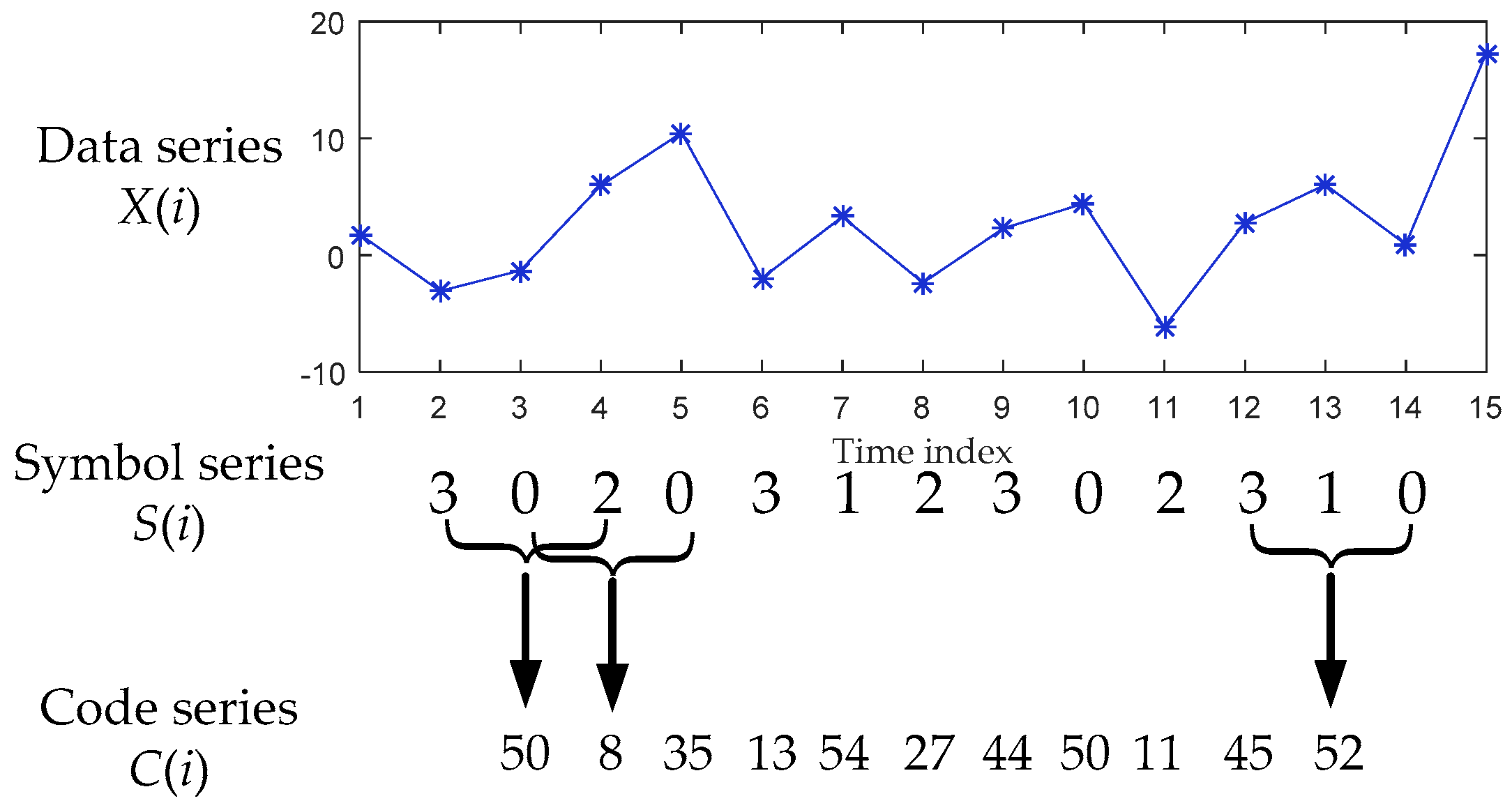
2.2. Differential Symbolic Entropy

2.2.1. Traditional Symbolization

Symbolization plays an important role in symbolic dynamic analysis. The symbolic procedure inevitably leads to the loss of part of statistical information; however, it simplifies time series analysis and contributes to dynamic complexity detection by extracting symbolic dynamic information.
A symbolization in the works of Kurths et al. [29], using typical local dynamic symbolization, conducts symbolic transformation by comparing relationships between adjacent symbols. Given univariate time series Y = { y i , i = 1 , , N } , traditional symbolization, being described as especially reflecting the dynamical properties of the record [29], transforms time series into a symbol sequence as Equation (7):
S i ( y i ) = { 0 : Δ y 1.5 σ Δ 1 : Δ y > 0   and   Δ y 1.5 σ Δ 2 : Δ y > 1.5 σ Δ   and   Δ y < 0   3 : Δ y 1.5 σ Δ
Traditional symbolic transformation refines the differences between neighboring elements, but it only considers two adjacent values and lacks flexibility due to the fixed 1.5 σ Δ .

2.2.2. Differential Symbolization

Taking the relationships of three consecutive elements into account, Yao et al. [17,18] proposed differential symbolic transformation with a flexible controlling parameter. The complexity detection of this symbolization is attributed to detailed local dynamic information. Considering univariate time series Y = { y i , i = 1 , , N } , the differences between the current element and its forward and backward ones are expressed as D 1 = y ( i ) y ( i 1 ) and D 2 = y ( i + 1 ) y ( i ) . The four-symbol differential symbolization with the controlling parameter α is obtained by the following formula:
S i ( y i ) = { 0 : d i f f α v a r 1 : 0 d i f f < α v a r 2 : α v a r < d i f f < 0 3 : d i f f α v a r
where d i f f = D 1 D 2 and v a r = ( D 1 2 + D 2 2 ) / 2 . The symbolization in Equation (8) takes advantage of more detailed local information of complexity measures than traditional symbolic transformation.
Construction of symbol sequences, or words, is the next step by collecting groups of symbols together in temporal order. This coding process is to create symbol templates or words with finite symbols and has some similarities to embedding theory for phase space construction [18]. The symbol sequence will be coded into m-bit series C ( i ) , and there are 4 m symbols in coded series considering the four-symbol differential symbolization. Taking 3-bit coding as an example, the code for ‘ α β γ ’ can be c ( i ) = α n 2 + β n + γ , where n = 4 . The procedure of symbolization and coding is illustrated in Figure 1. The probability of each code symbol is P ( π ) = [ p ( π 1 ) , p ( π 2 ) , , p ( π 4 m ) ] .
Finally, DSE is obtained by computing the Shannon entropy from the probability distribution for all the words, and then, it is normalized by its highest value, i.e., log 2 4 m , such that:
D S E = 1 log 2 4 m p ( π i ) log 2 p ( π i ) ,   where   p ( π i ) 0

2.3. Mutual Information

Originating from the classic and profoundly influential work by Shannon, the MI between discrete random variables X and Y is defined as [30]:
M I ( X ; Y ) = y Y x X p ( x , y ) log ( p ( x , y ) p ( x ) p ( y ) )
where p ( x , y ) is the joint probability distribution function of x and y, p ( x ) and p ( y ) are the marginal probability distribution functions of x and y, respectively.
The MI of continuous random variables can be expressed as a double integral [31]:
M I ( X ; Y ) = Y X p ( x , y ) log ( p ( x , y ) p ( x ) p ( y ) ) d x d y
In probability theory and information theory, the mutual information of two random variables represents a measure of the interdependence of variables. If X and Y are independent, M I ( X ; Y ) = 0 .
Furthermore, the MI can also be expressed as [31]:
M I ( X ; Y ) = H ( X ) H ( X | Y ) = H ( Y ) H ( Y | X ) = H ( X ) + H ( Y ) H ( X , Y ) = H ( X , Y ) H ( X | Y ) H ( Y | X )
where H ( X ) and H ( Y ) are information entropy, H ( X | Y ) and H ( Y | X ) are conditional entropy, and H ( X , Y ) is the joint entropy of X and Y.
Assume that the original signal x ( t ) is decomposed by RPSEMD to obtain K IMFs (for convenience, the residue r ( t ) is counted as the last IMF), which are denoted as I M F 1 ( t ) , I M F 2 ( t ) , …, I M F i ( t ) , …, I M F K ( t ) , respectively. Therefore, the normalized MI (norMI) between the ith IMF and the original signal can be expressed as:
n o r M I ( I M F i ; y ( t ) ) = M I ( I M F i ; y ( t ) ) m = 1 K M I ( I M F m ; y ( t ) ) ,   i = 1 , 2 , , K
For convenience, the norMI used in the following test represents the norMI between the IMF and the original signal, unless otherwise specified.

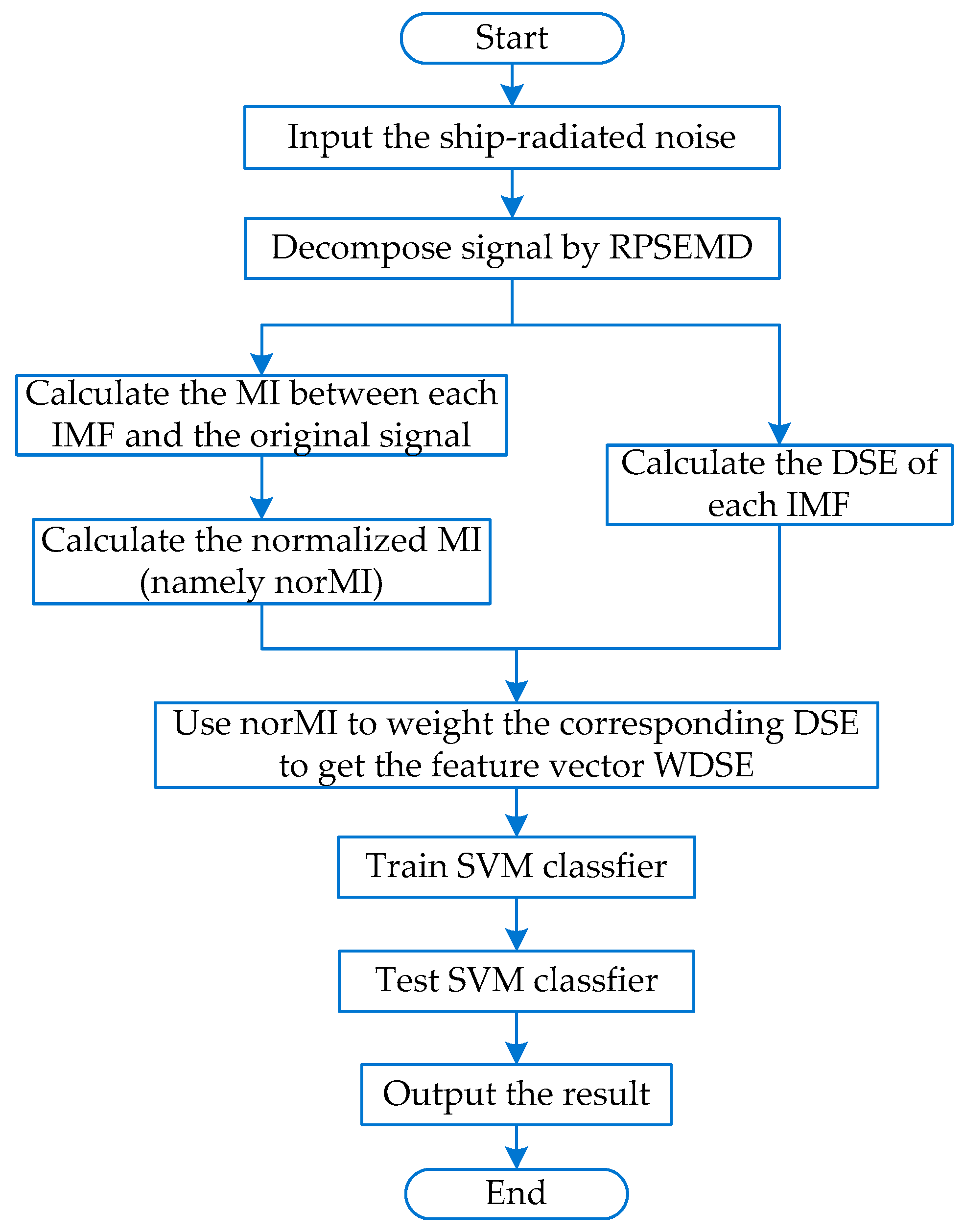
3. The Proposed Feature Extraction Method

The flowchart of the proposed feature extraction method is shown in Figure 2.
Step 1.
The three types of recorded ship-radiated noise are normalized.
Step 2.
The ship-radiated noise is decomposed into a series of IMFs by RPSEMD.
Step 3.
Calculate the DSE of each IMF.
Step 4.
The MIs between each IMF and the original signal are calculated, and then, the sum of all MIs is used as the denominator to calculate the normalized value of each MI, expressed as norMI.
Step 5.
The norMI is used as the weight coefficient to weight the corresponding DSE, and the feature vector WDSE is obtained.
Step 6.
The feature vector WDSE is input into the support vector machine for classification.

4. Analysis of the Simulation Signal

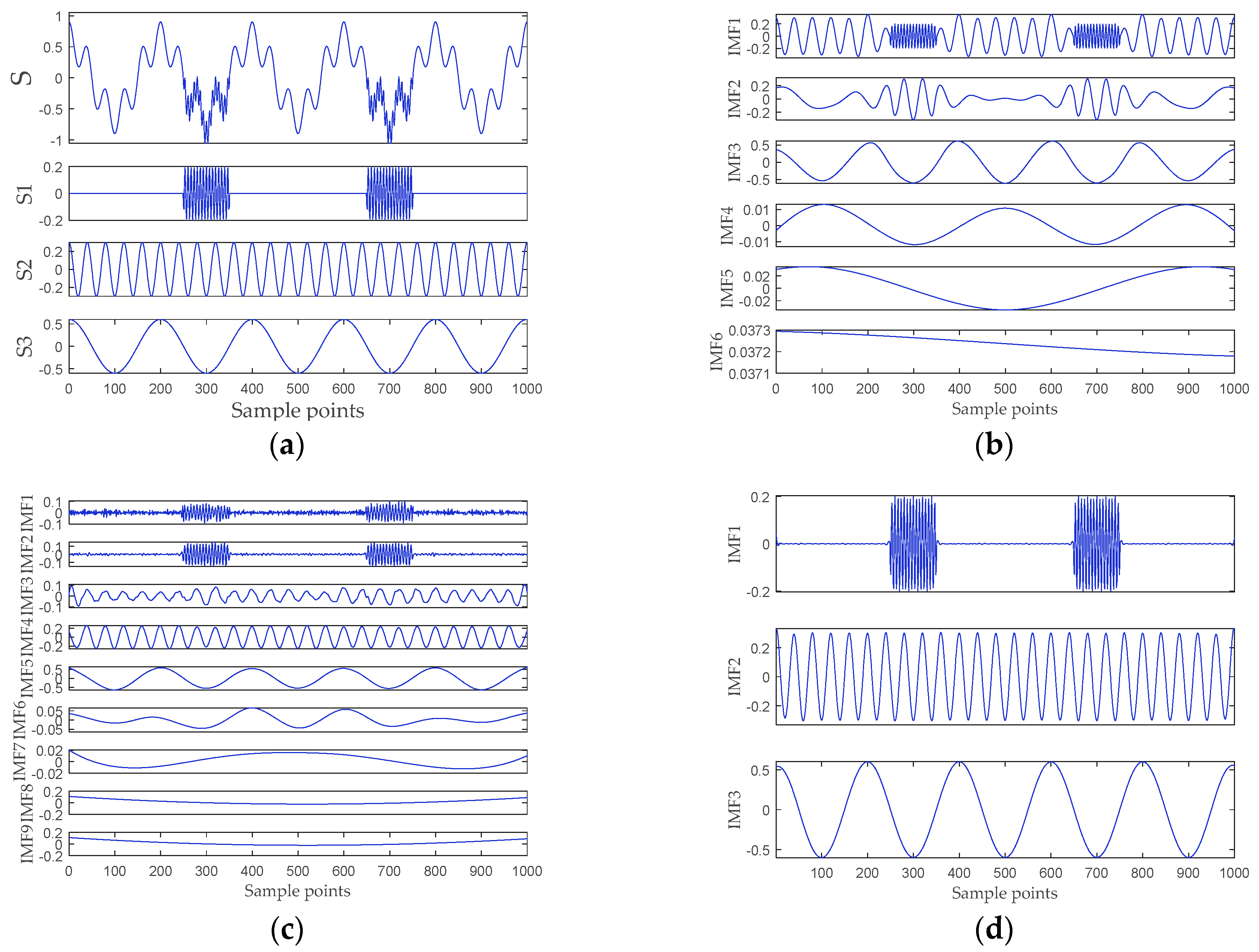
4.1. Performance Analysis of EMD, EEMD, and RPSEMD

To verify that RPSEMD can alleviate the mode mixing problem, we give an example here. The simulation signals are as follows:
s 1 = { 0 ,   0 n < 0.25 0.2 cos ( 300 π n ) ,   0.25 n < 0.35 0 ,   0.35 n < 0.65 0.2 cos ( 300 π n ) ,   0.65 n < 0.75 0 ,   0.75 n 1
s 2 = 0.3 cos ( 50 π n ) ,   0 n 1
s 3 = 0.6 cos ( 10 π n ) ,   0 n 1
S = s 1 + s 2 + s 3
where s 1 , s 2 , and s 3 represent the three components of S , and the sampling frequency is 10 kHz. EMD, EEMD, and PRSEMD are used to decompose S . The simulation signals and the decomposition results are presented in Figure 3. According to the literature [26], the amplitude of the noise is set as 0.3, and the ensemble size is 100 for the EEMD method. It can be seen from Figure 3b that the IMF1 and IMF2 of the EMD have obvious mode mixing. EEMD alleviates the mode mixing to a certain extent, but the original signal is decomposed into nine mode components, of which IMF6–IMF9 have no practical physical meaning. Compared with EEMD, there is no need to select parameters for RPSEMD, so it has better practicability. Figure 3d manifests that the original signal is decomposed into three IMFs by PRSEMD, and these IMFs are very close to the three components of the original signal. Consequently, compared with EMD and EEMD, RPSEMD better optimizes the mode mixing problem. Further, the energy of the signal can be calculated by:
E = i = 1 N p i 2
where N represents the length of the signal and p i denotes the amplitude of the ith sample point. The energy of simulation signals and IMFs is shown in Table 1 and Table 2, respectively. It can be seen that the energy of the IMFs of RPSEMD is equal to the simulation signal. The results demonstrate that it is feasible to use RPSEMD as the signal decomposition method in this paper.

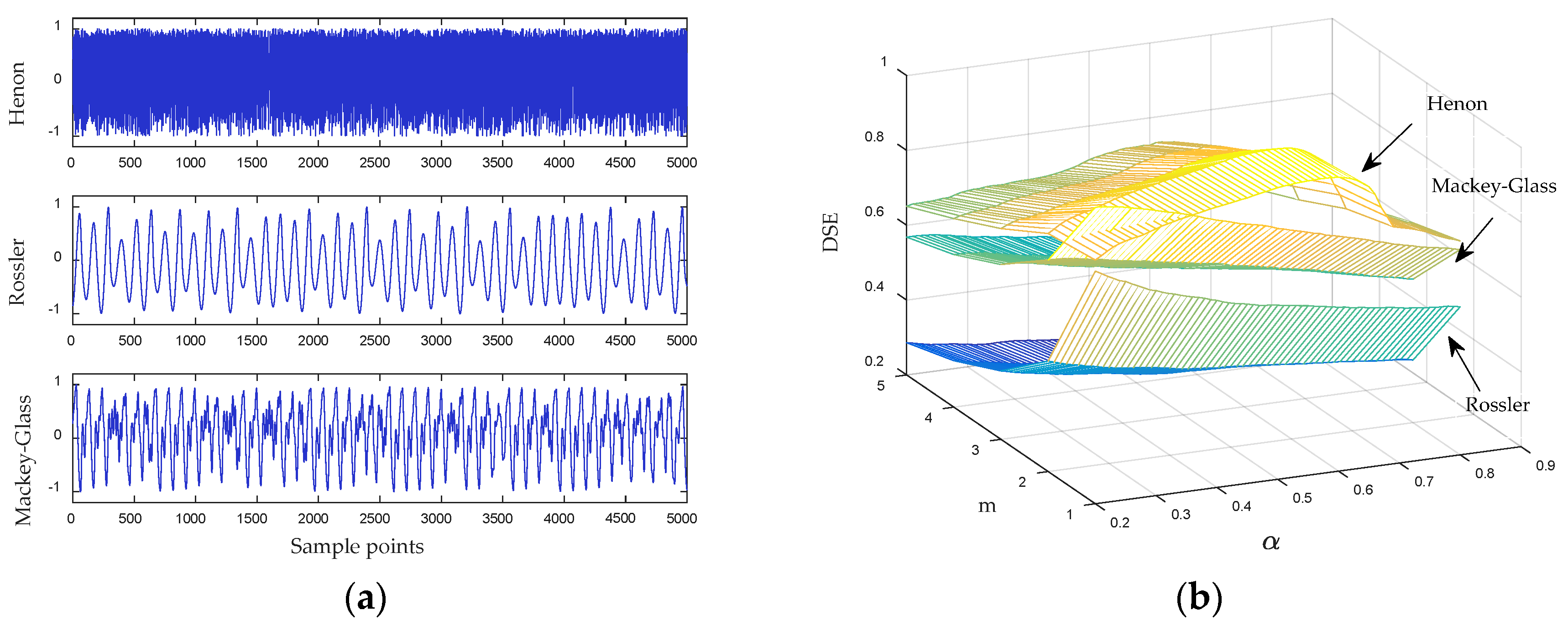
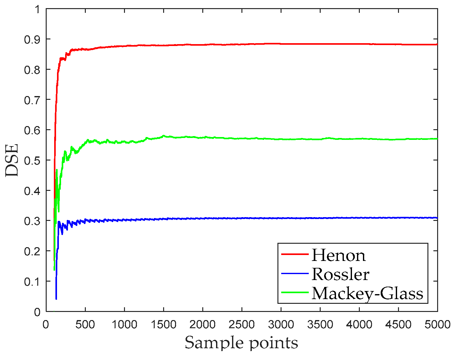
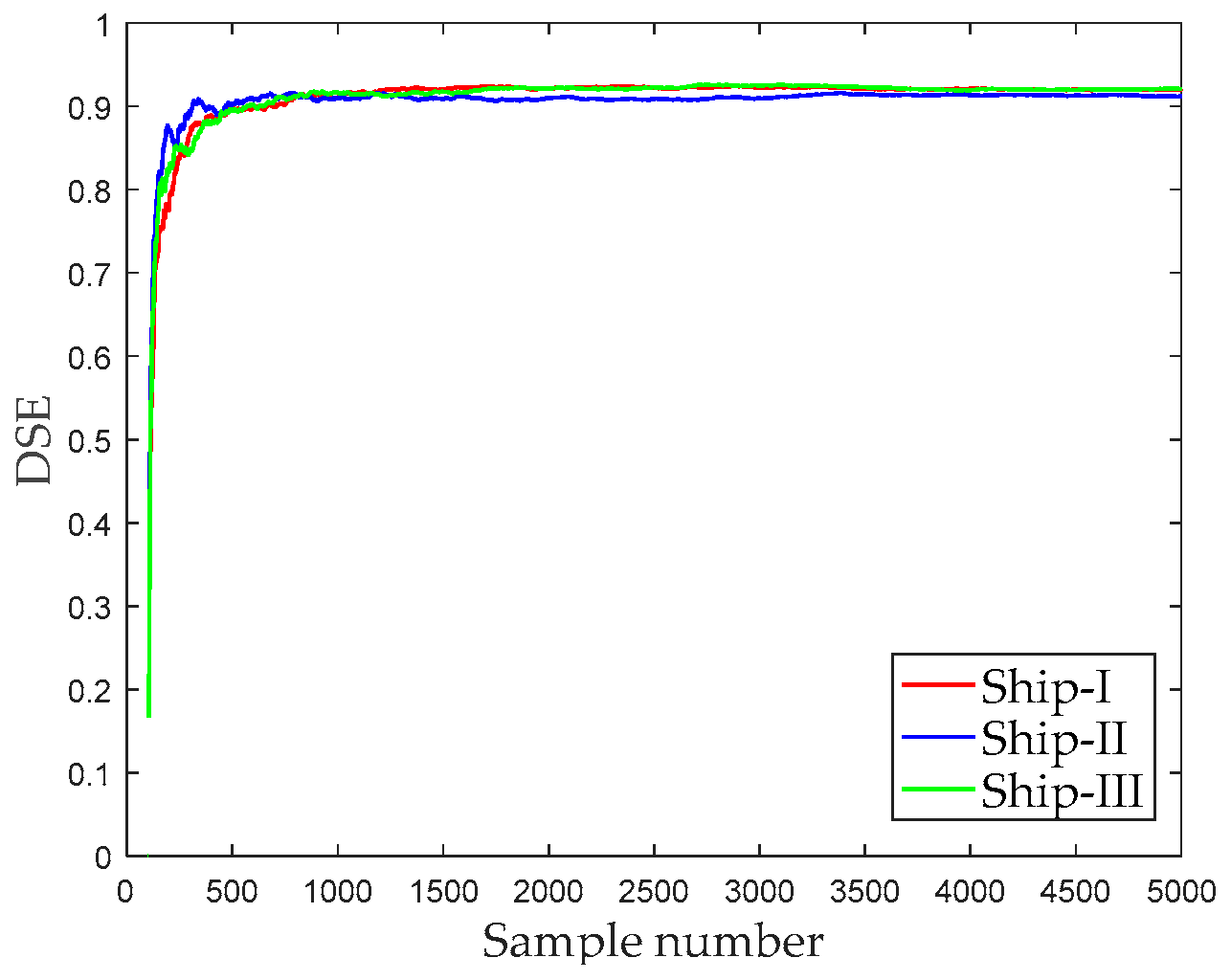
4.2. Parameter Selection of DSE

Ship-radiated noise has obvious chaotic characteristics. In order to analyze the influence of DSE parameters on the entropy value, three typical chaotic signals are selected for simulation experiments. These chaotic signals can be expressed as follows [32]:
(1)
Henon mapping: { x ( n + 1 ) = 1 1.4 x ( n ) 2 + y ( n ) y ( n + 1 ) = 0.3 x ( n ) , and the initial condition is { x 0 = 0 y 0 = 0 . In this paper, we analyze the data points in the y-direction.
(2)
Rossler system: { x ˙ = ( y + z ) y ˙ = x + 0.2 y z ˙ = 0.2 + z ( x 5 ) , the initial condition is { x 0 = 1 y 0 = 0 z 0 = 1 , and the integral step size is 0.05. In this paper, we analyze the data points in the x-direction.
(3)
Mackey–Glass signal: d x d t = b x ( t ) + a x ( t 30 ) 1 + x 10 ( t 30 ) , where { a = 0.2 b = 0.1 .
The original signals are taken from 5000 points of the above three types of simulation signals. The original signals are normalized to get the time-domain waveform shown in Figure 4a. We select different DSE parameters to calculate the entropy of simulated signals. In this section, we mainly study the influence of symbol length m and the adjustment factor α on the differential symbolic entropy. The symbol length is set from 1–5 with a step size of one, and the adjustment factor is set from 0.1–0.8 with a step size of 0.01. The DSE entropy under different parameters is shown in Figure 4b.
It can be seen from Figure 4b that when m is equal to one, the entropy of the three types of chaotic signals is closest. When m is greater than one, these signals can be better distinguished. When m is fixed, the value of α has no significant effect on the entropy of the Rossler signal and the Mackey–Glass signal. For the Henon mapping, as α increases, its entropy increases first and then decreases, and the maximum is obtained around 0.6. In conclusion, the value of m has little influence on DSE. When α is equal to 0.6, DSE can be used to classify the three types of chaotic signals better. Considering the calculation speed and the stability of DSE, we set m and α to three and 0.6, respectively.
It can also be seen from Figure 4b that the Henon mapping has the largest DSE entropy, which means it is more complex. The DSE of the Rossler signal are minimum, which means that the Rossler signal has regularity to some extent. The DSE of the Mackey–Glass signal are a bit lower than those of the Henon map, indicating that the Mackey–Glass signal also has higher complexity. The results demonstrate that DSE can discriminate the different simulation signals and can be used to quantify the information content of nonlinear time series.
To illustrate the influence of sampling points on entropy, we calculate DSE at different sampling points. Figure 5 shows the DSE under the different data points of these signals; when the number of sampling points is less than 500, the DSE fluctuates greatly; when the number of sampling points is greater than 500, the DSE is more stable. Therefore, when the number of sampling points of the signal is greater than 500, the result of DSE is reliable.

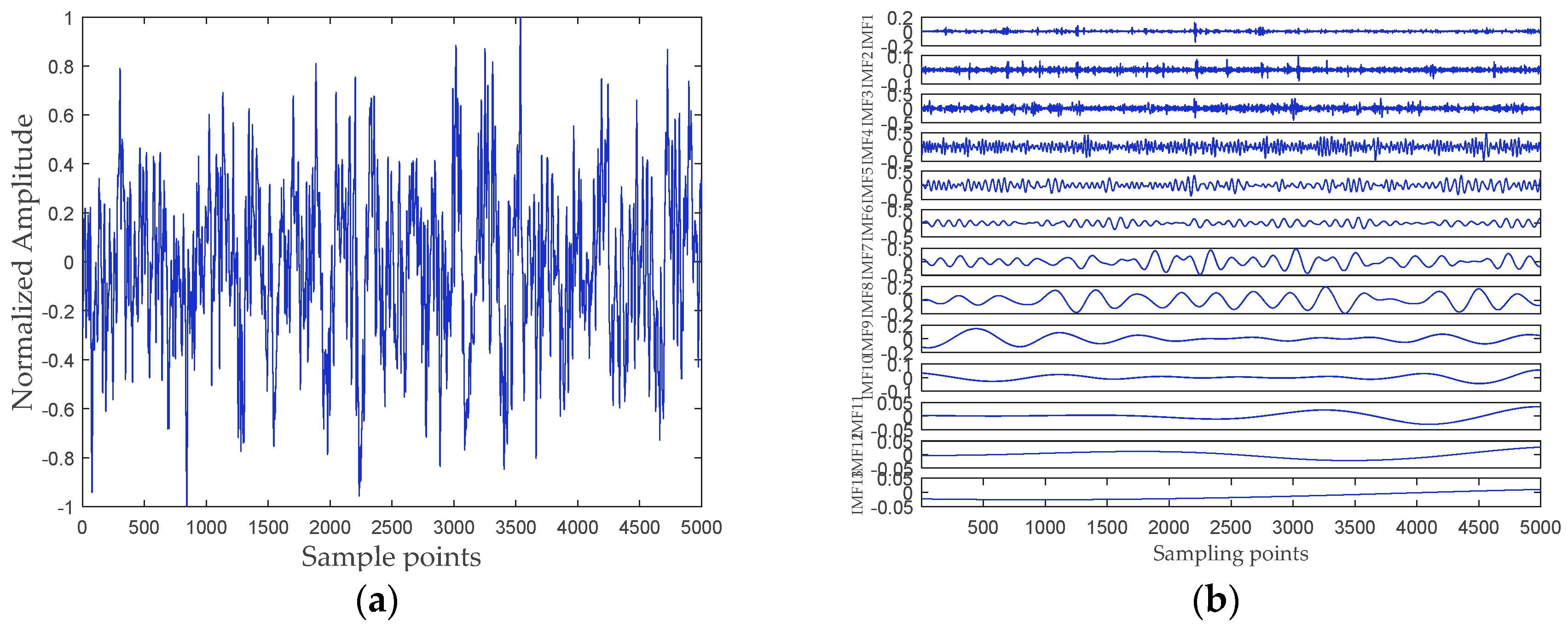
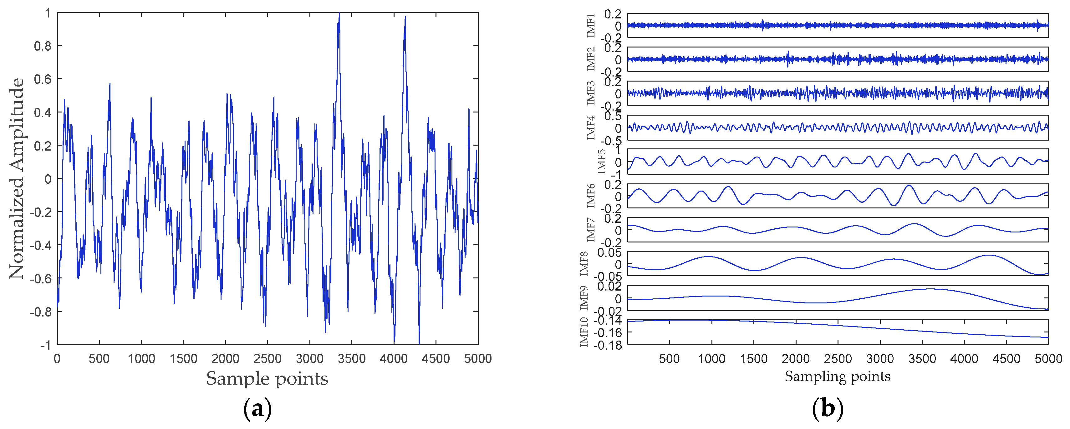
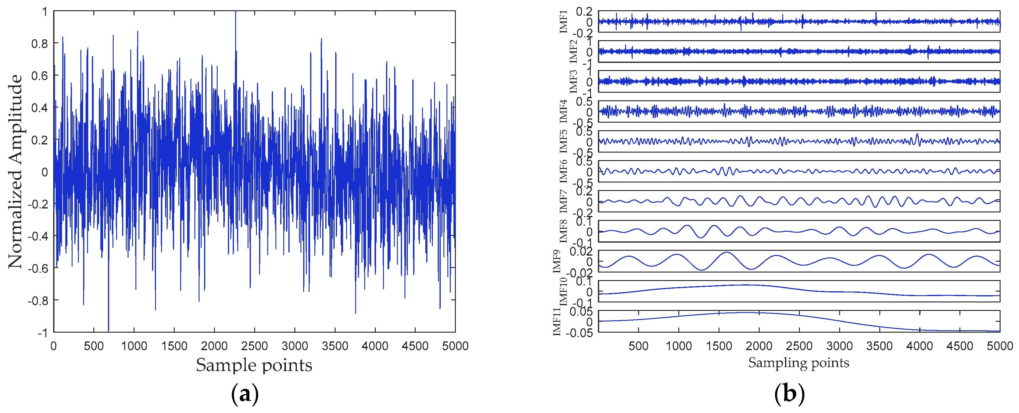
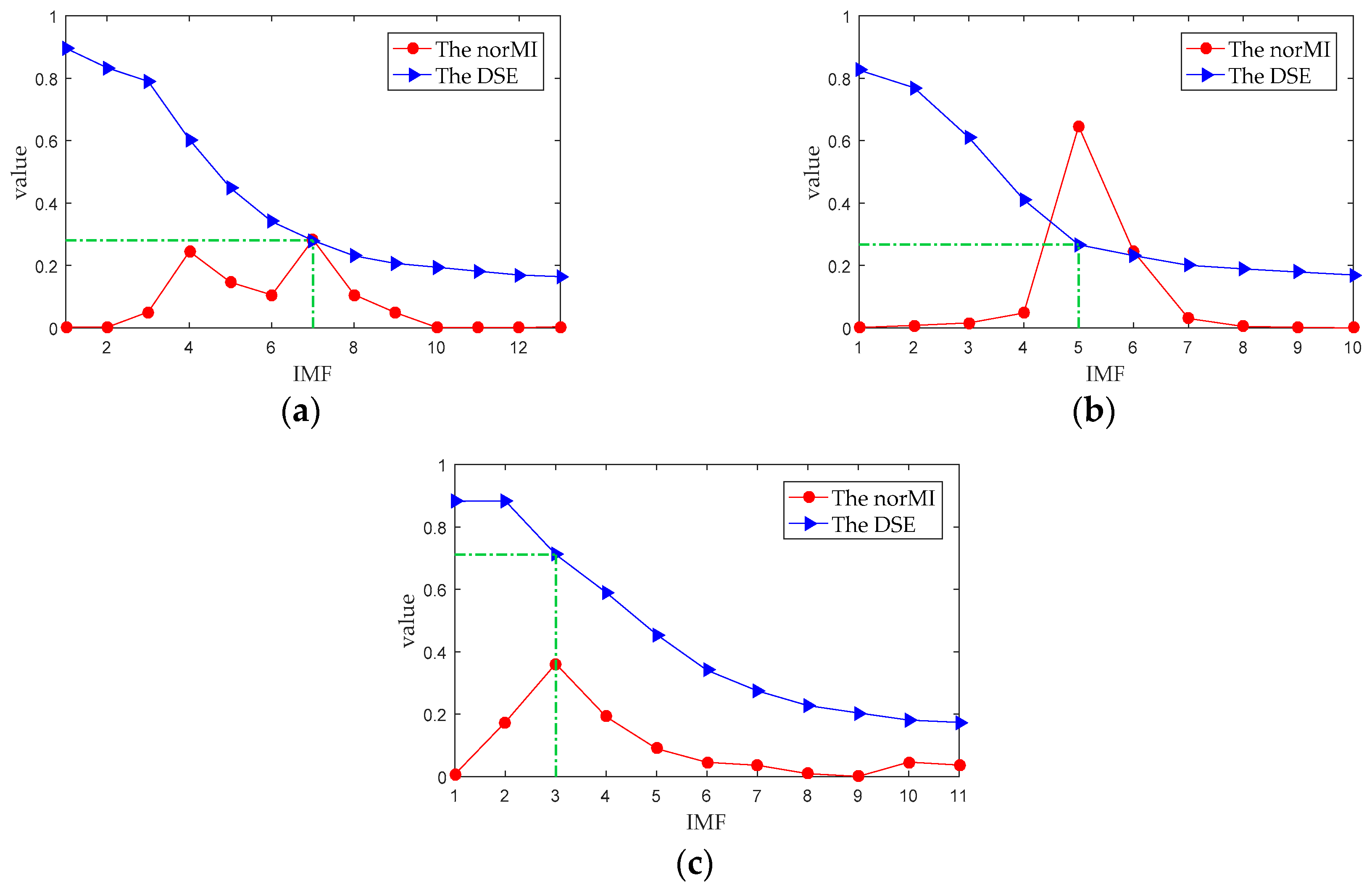
5. Analysis of Ship-Radiated Noise Based on RPSEMD, MI, and DSE

In this paper, all data of ship-radiated noise come from the official website of the National Park Service (available at http://www.nps.gov/glba/naturescience/soundclips.htm). Three different types of ship-radiated noise are selected as sample data, namely ferry, cruise ship, and freighter. For convenience, we named the three ship-radiated noise as Ship-I, Ship-II, and Ship-III, respectively. Each type of underwater acoustic signals has 30 sample data. Each sample length is 5000 points, and the sampling frequency is 44.1 kHz. The samples are normalized to get the time-domain waveform of three types of ship-radiated noise shown in Figure 6a, Figure 7a and Figure 8a, respectively. The abscissa represents the sampling point, and the ordinate represents the normalized amplitude. The RPSEMD decomposition results of the three types of ship-radiated noise are shown in Figure 6b, Figure 7b and Figure 8b, respectively.
Figure 9 shows the DSE of different sampling point numbers, whose entropy gradually stabilizes with the increase of the number of sampling points. When the number of sampling points reaches 500, the DSE entropy of the three types of ships-radiated noise are stable at around 0.9. It can be found that DSE is sensitive to noise, so these signals have a large entropy. Therefore, it is difficult to distinguish these three types of ships if the DSE of the original signal is directly used as the feature vector.
It can be seen from Figure 6b, Figure 7b and Figure 8b that the ship-radiated noise is decomposed into a series of IMFs by RPSEMD, and the frequency of the IMF decreases sequentially with the order of the modes. For different ship-radiated noise, the number of IMFs decomposed by RPSEMD is different. The norMI and DSE for each ship-radiated noise are listed in Figure 10.
In Figure 10, the abscissa represents the IMF ordinal number of ship-radiated noise, the red circle represents the norMI of IMF, and the blue triangle represents the DSE of IMF. It can be found that DSE decreases with the increase of IMF, indicating that the higher the order of IMF, the lower the complexity. Consequently, if only DSE is used as the feature vector, it is arduous to distinguish the three types of ship-radiated noise.
Li et al. [21] used the IMF with the highest energy as the principal IMF (PIMF) and used the permutation entropy of PIMF as the feature vector (namely EMD-PIMF-PE) to realize the classification of three types of ship-radiated noise. In Figure 10, the DSE of the IMF with the largest norMI is marked with a green dashed line, and the DSE of the IMF with the largest norMI is also listed in Table 3. It can be seen that for Ship-I and Ship-II, the DSE of the IMF with the largest norMI are around 0.27, and the values are quite close. Therefore, it may be arduous to distinguish between Ship-I and Ship-II using this method, which will be proven later.
Therefore, we consider using norMI as the weight, weighting the corresponding DSE and using the sum of the weighted DSE (WDSE) as the feature vector, giving the formula as follows:
W D S E = i = 1 K n o r M I i D S E i
where n o r M I i represents the norMI of the ith IMF, D S E i denotes the DSE of the ith IMF, and K is the number of IMFs. The WDSE of the three ships’ radiated noise are listed in Table 4. It can be found that the difference between the feature vectors of Ship-I and Ship-II becomes larger.

6. Feature Extraction and Classification of Ship-Radiated Noise

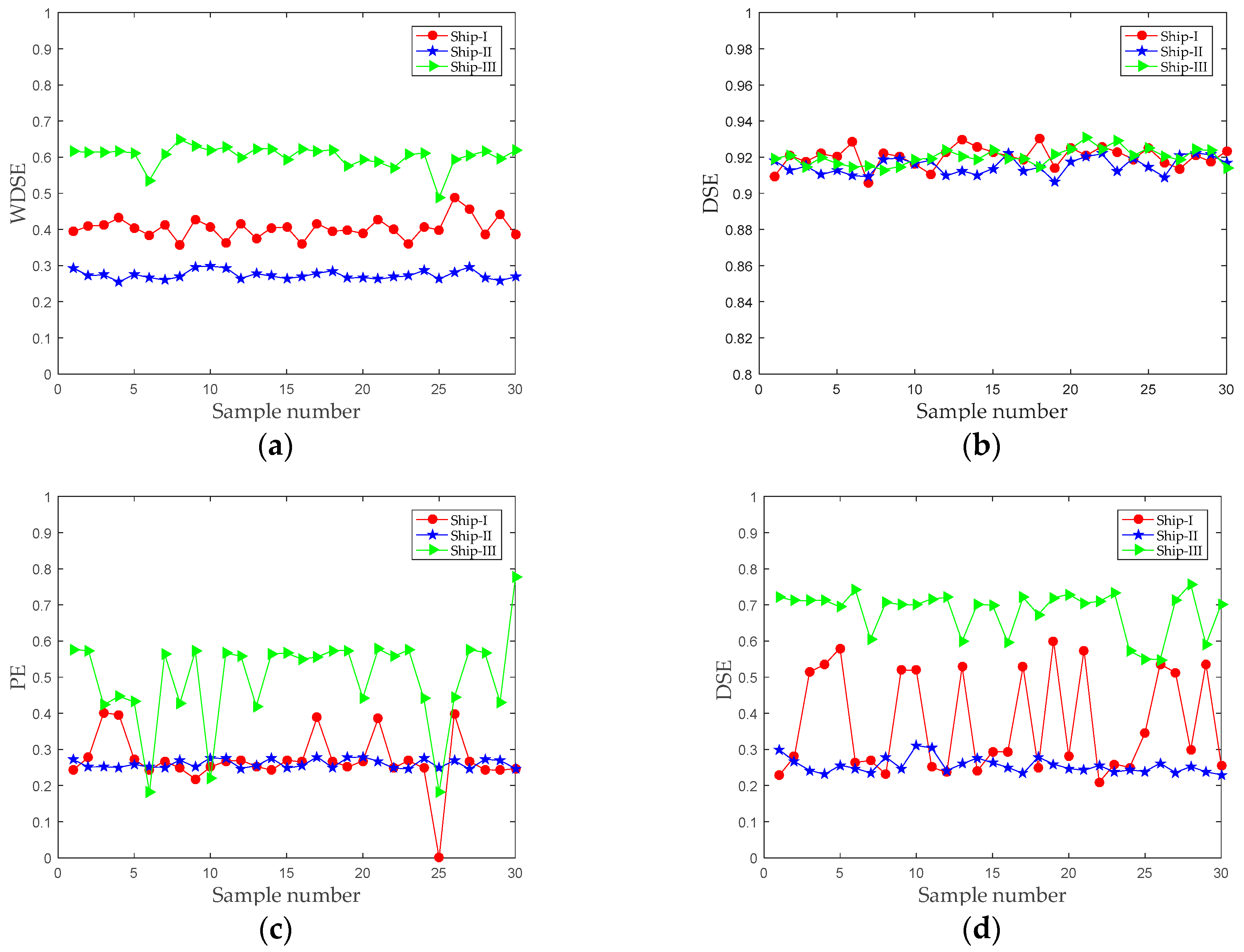
6.1. Feature Extraction
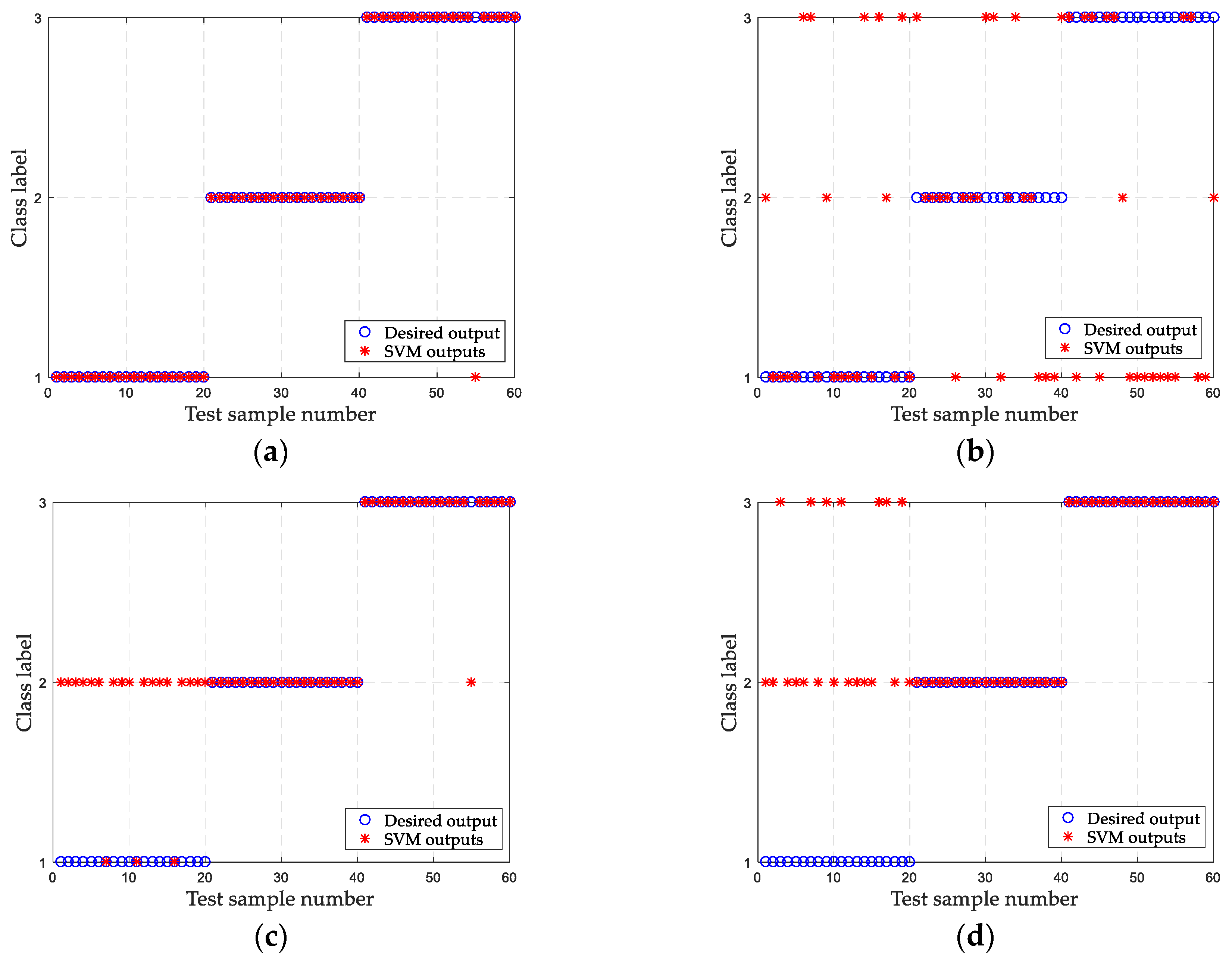
To verify the effectiveness of the proposed feature extraction method, 30 samples of each type of ship-radiated noise are selected. The WDSE distribution of the three types of ship-radiated noise is shown in Figure 11a. The abscissa represents the number of samples, and the ordinate represents the feature vector WDSE. It can be seen that the WDSE of Ship-III is the largest, and the WDSE of Ship-II is the smallest. The results demonstrate that the WDSE value is at the same level for the same ships, but there is an obvious difference for different types of ships. The above results manifest that the proposed feature extraction method can distinguish three types of ship-radiated noise.
In order to prove the superiority of the proposed method, the DSE of original ship-radiated noise, the EMD-PIMF-PE method [21], and the DSE of the IMF with the largest norMI (IMF-norMI-DSE) are taken as the feature vector of ship-radiated noise, respectively. According to literature [21], the embedding dimension and time delay of permutation entropy are set as four and one, respectively. As shown in Figure 11b, due to the influence of the marine environment, the DSEs of the three types of ship-radiated noise are basically between 0.9 and 0.94. Therefore, it is not feasible to distinguish these ships directly by using DSE. It can be seen from Figure 11c that the EMD-PIMF-PE method can basically distinguish between Ship-II and Ship-III, but there is a large overlap between Ship-I and Ship-II. Figure 11c,d have similar results. It can be seen that the feature vector of Ship-III is the largest, and the feature vector of Ship-II is the smallest. This result is consistent with the proposed method in this paper. Compared with the proposed method, the IMF-norMI-DSE method is completely unable to identify Ship-I because their DSE values fluctuate greatly.

6.2. Classification

To realize the automatic identification of ship-radiated noise, the extracted features are input into the SVM for training and testing. For each type of ship-radiated noise, 10 samples are used as training samples, and the remaining 20 samples are used as test samples. To compare classification accuracy, the DSE of the original ship-radiated noise, the EMD-PIMF-PE method [21], and the IMF-norMI-DSE method are also used to classify ship-radiated noise. The SVM outputs of these four methods are shown in Figure 12, respectively, and the recognition rates are listed in Table 5. It can be found that the classification results of SVM are consistent with the feature extraction results in Section 6.1. For each type of ship-radiated noise, the DSE of the original signal is not completely classified correctly, and the classification accuracy is 48.3333%. The EMD-PIMF-PE method can classify Ship-II and Ship-III well, but cannot correctly identify Ship-I, and the classification accuracy is 70%. The IMF-norMI-DSE method is inferior to the EMD-PIMF-PE method, and the classification accuracy is 66.6667%. Compared with the other three methods, the classification accuracy of the proposed method reaches 98.3333%. The results indicate that the proposed method can better classify the three types of ship-radiated noise.

7. Conclusions

To improve the recognition accuracy of ship-radiated noise, a novel feature extraction method based on RPSEMD, MI, and DSE is proposed. The main findings in this paper are highlighted as follows:
(1)
A novel differential symbolic entropy for measuring the complexity of time series is introduced. DSE not only has the advantage of high computational efficiency, but also has a significant effect on shorter time series. It was first applied to underwater acoustic signal processing.
(2)
Simulation experiments demonstrate that RPSEMD can better alleviate the mode mixing problem compared with EMD and EEMD. Therefore, this paper uses RPSEMD as a signal decomposition tool.
(3)
Compared with [21], it is often the case that only one IMF with the principal features is selected for feature extraction. In this paper, the entropy is weighted by norMI, so the importance of each IMF is considered.
(4)
The method proposed in this paper can extract the characteristics of ship-radiated noise more precisely and comprehensively, and the classification accuracy reaches 98.3333%.
Last but not least, this paper provides a new idea for feature extraction of nonlinear and non-stationary signals. For example, the weight coefficient can be replaced by the IMF’s energy and other parameters. It is worth noting that although both EEMD and RPSEMD improve the mode mixing problem of EMD, RPSEMD is more efficient than EEMD and therefore has better utility. In the following work, we will use RPSEMD to reduce noise of underwater acoustic signal and compare it with EEMD.

Author Contributions

G.L., Z.Y., and H.Y. conceived of the idea and research theme. Z.Y. designed and performed the experiments. G.L., Z.Y., and H.Y. analyzed the experimental results. G.L., Z.Y., and H.Y. wrote and revised the paper.

Funding

This work was supported by the National Natural Science Foundation of China (No. 51709228) and the Innovation Funds of the Graduate Programs of Xi’an University of Posts and Telecommunications (No. CXJJ2017022).

Acknowledgments

We thank the anonymous reviewers for their constructive comments, which improved the quality of this paper.

Conflicts of Interest

The authors declare no conflict of interest.

References

  1. Siddagangaiah, S.; Li, Y.; Guo, X.; Yang, K. On the dynamics of ocean ambient noise: Two decades later. Chaos 2015, 25, 103117. [Google Scholar] [CrossRef] [Green Version]
  2. Zheng, S.; Guo, H.; Li, Y.; Wang, B.; Zhang, P. A new method for detecting line spectrum of ship-radiated noise using duffing oscillator. Chin. Sci. Bull. 2007, 52, 1906–1912. [Google Scholar] [CrossRef]
  3. Li, Y.; Li, Y.; Chen, X.; Yu, J. Research on ship-radiated noise denoising using secondary variational mode decomposition and correlation coefficient. Sensors 2018, 18, 48. [Google Scholar] [CrossRef]
  4. Wales, S.C.; Heitmeyer, R.M. An ensemble source spectra model for merchant ship-radiated noise. J. Acoust. Soc. Am. 2002, 111, 1211–1231. [Google Scholar] [CrossRef]
  5. Li, G.; Yang, Z.; Yang, H. Noise reduction method of underwater acoustic signals based on uniform phase empirical mode decomposition, amplitude-aware permutation entropy, and Pearson correlation coefficient. Entropy 2018, 20, 918. [Google Scholar] [CrossRef]
  6. Chen, Z.; Li, Y.; Liang, H.; Yu, J. Hierarchical cosine similarity entropy for feature extraction of ship-radiated noise. Entropy 2018, 20, 425. [Google Scholar] [CrossRef]
  7. Wang, S.; Zeng, X. Robust underwater noise targets classification using auditory inspired time-frequency analysis. Appl. Acoust. 2014, 78, 68–76. [Google Scholar] [CrossRef]
  8. Li, Y.; Li, Y.; Chen, X.; Yu, J. A novel feature extraction method for ship-radiated noise based on variational mode decomposition and multi-scale permutation entropy. Entropy 2017, 19, 342. [Google Scholar] [CrossRef]
  9. Huang, N.E.; Shen, Z.; Long, S.R.; Wu, M.C.; Shih, H.H.; Zheng, Q.A.; Yen, N.; Tung, C.C.; Liu, H.H. The empirical mode decomposition and the Hilbert spectrum for nonlinear and non-stationary time series analysis. Proc. R. Soc. Lond. 1998, 454, 903–995. [Google Scholar] [CrossRef]
  10. Wu, Z.; Huang, N.E. Ensemble empirical mode decomposition: A noise-assisted data analysis method. Adv. Adapt. Data Anal. 2009, 1, 1–41. [Google Scholar] [CrossRef]
  11. Wang, C.; Qian, K.; Da, F. Regenerated phase-shifted sinusoid-assisted empirical mode decomposition. IEEE Signal Process. Lett. 2016, 23, 556–560. [Google Scholar] [CrossRef]
  12. Yi, C.; Lv, Y.; Xiao, H.; You, G.; Dang, Z. Research on the blind source separation method based on regenerated phase-shifted sinusoid-assisted EMD and its application in diagnosing rolling-bearing faults. Appl. Sci. 2017, 7, 414. [Google Scholar] [CrossRef]
  13. Lake, D.E.; Richman, J.S.; Griffin, M.P.; Moorman, J.R. Sample entropy analysis of neonatal heart rate variability. Am. J. Physiol. Regul. Integr. Comp. Physiol. 2002, 283, 789. [Google Scholar] [CrossRef] [PubMed]
  14. Bandt, C.; Pompe, B. Permutation entropy: A natural complexity measure for time series. Phys. Rev. Lett. 2002, 88, 174102. [Google Scholar] [CrossRef] [PubMed]
  15. Aziz, W.; Arif, M. Complexity analysis of stride interval time series by threshold dependent symbolic entropy. Eur. J. Appl. Physiol. 2006, 98, 30–40. [Google Scholar] [CrossRef] [PubMed]
  16. Azami, H.; Escudero, J. Amplitude-aware permutation entropy: Illustration in spike detection and signal segmentation. Comput. Meth. Progr. Biomed. 2016, 128, 40–51. [Google Scholar] [CrossRef] [PubMed] [Green Version]
  17. Yao, W.; Wang, J. Double symbolic joint entropy in nonlinear dynamic complexity analysis. AIP Adv. 2017, 7, 075313. [Google Scholar] [CrossRef] [Green Version]
  18. Yao, W.; Wang, J. Differential symbolic entropy in nonlinear dynamics complexity analysis. physics.data-an (under review). arXiv, 2019; arXiv:1801.08416v2. [Google Scholar]
  19. Yang, L. A empirical mode decomposition approach to feature extraction of ship-radiated noise. In Proceedings of the 2009 4th IEEE Conference on Industrial Electronics and Applications, Xi’an, China, 25–27 May 2009; pp. 3682–3686. [Google Scholar] [CrossRef]
  20. Bao, F.; Wang, X.; Tao, Z.; Wang, Q.; Du, S. EMD-based extraction of modulated cavitation noise. Mech. Syst. Signal Process. 2010, 24, 2124–2136. [Google Scholar] [CrossRef]
  21. Li, Y.; Li, Y.; Chen, Z.; Chen, X. Feature extraction of ship-radiated noise based on permutation entropy of the intrinsic mode function with the highest energy. Entropy 2016, 18, 393. [Google Scholar] [CrossRef]
  22. Zhou, S.; Qian, S.; Chang, W.; Xiao, Y.; Cheng, Y. A novel bearing multi-fault diagnosis approach based on weighted permutation entropy and an improved SVM ensemble classifier. Sensors 2018, 18, 1934. [Google Scholar] [CrossRef] [PubMed]
  23. Bao, F.; Li, C.; Wang, X.; Wang, Q.; Du, S. Ship classification using nonlinear features of radiated sound: An approach based on empirical mode decomposition. J. Acoust. Soc. Am. 2010, 128, 206–214. [Google Scholar] [CrossRef] [PubMed]
  24. Gan, X.; Lu, H.; Yang, G.; Liu, J. Rolling bearing diagnosis based on composite multiscale weighted permutation entropy. Entropy 2018, 20, 821. [Google Scholar] [CrossRef]
  25. Knobles, D.P. Maximum entropy inference of seabed attenuation parameters using ship, radiated broadband noise. J. Acoust. Soc. Am. 2015, 138, 3563–3575. [Google Scholar] [CrossRef] [PubMed]
  26. Yang, H.; Li, Y.; Li, G. Energy analysis of ship radiated noise based on ensemble empirical mode decomposition. J. Vib. Shock 2015, 34, 55–59. [Google Scholar] [CrossRef]
  27. Firat, U.; Akgul, T. Compressive sensing for detecting ships with second-order cyclostationary signatures. IEEE J. Ocean. Eng. 2018, 43, 1086–1098. [Google Scholar] [CrossRef]
  28. Rilling, G.; Flandrin, P. One or two frequencies? the empirical mode decomposition answers. IEEE Trans. Signal Process. 2008, 56, 85–95. [Google Scholar] [CrossRef]
  29. Kurths, J.; Voss, A.; Saparin, P.; Witt, A.; Kleiner, H.J.; Wessel, N. Quantitative analysis of heart rate variability. Chaos 1995, 5, 88–94. [Google Scholar] [CrossRef] [Green Version]
  30. Li, Y.; Li, Y.; Chen, X.; Yu, J.; Yang, H.; Wang, L. A new underwater acoustic signal denoising technique based on CEEMDAN, mutual information, permutation entropy, and wavelet threshold denoising. Entropy 2018, 20, 563. [Google Scholar] [CrossRef]
  31. Peng, H.; Long, F.; Ding, C. Feature selection based on mutual information criteria of max-dependency, max-relevance, and min-redundancy. IEEE Trans. Pattern Anal. 2005, 27, 1226–1238. [Google Scholar] [CrossRef] [Green Version]
  32. Fan, C.; Fan, Qi.; Li, H. Base-scale entropy and energy analysis of flow characteristics of the two-phase flow. Syst. Sci. Control Eng. 2018, 6, 262–269. [Google Scholar] [CrossRef]
Figure 1. Process of symbolization and coding (data and symbols in virtual frame will not be symbolized or encoded). In the creation of code series, symbol length m is three. The first and last elements will not be transformed according to the determination of symbolization, and the last n − 1 bit symbols are not encoded for this encoding process.
Entropy 21 00176 g001
Figure 2. The flowchart of the proposed method. RPSEMD, regenerated phase-shifted sinusoid-assisted empirical mode decomposition; IMF, intrinsic mode function; WDSE, weighted differential symbolic entropy.
Entropy 21 00176 g002
Figure 3. The simulation signals and the decomposition result of EMD, ensemble EMD (EEMD), and RPSEMD. (a) The simulation signals; (b) the decomposition result of EMD; (c) the decomposition result of EEMD; and (d) the decomposition result of RPSEMD.
Entropy 21 00176 g003
Figure 4. (a) The normalized simulation signals and (b) DSE values of three types of simulated signals under different parameters.
Entropy 21 00176 g004
Figure 5. The DSE under the different data points of four simulation signals.
Entropy 21 00176 g005
Figure 6. (a) The time-domain waveform of Ship-I; and (b) the decomposition result of RPSEMD.
Entropy 21 00176 g006
Figure 7. (a) The time-domain waveform of Ship-II; and (b) the decomposition result of RPSEMD.
Entropy 21 00176 g007
Figure 8. (a) The time-domain waveform of Ship-III; and (b) the decomposition result of RPSEMD.
Entropy 21 00176 g008
Figure 9. The influence of sampling point number on DSE.
Entropy 21 00176 g009
Figure 10. The norMI and DSE of the IMFs. (a) Ship-I; (b) Ship-II; and (c) Ship-III.
Entropy 21 00176 g010
Figure 11. Feature extraction results of different methods. (a) The proposed method; (b) The DSE of original ship-radiated noise; (c) The EMD-PIMF-PE method; and (d) The IMF-norMI-DSE method.
Entropy 21 00176 g011
Figure 12. SVM classification results of different methods. (a) The proposed method; (b) the DSE of original ship-radiated noise; (c) the EMD-PIMF-PE method; and (d) the IMF-norMI-DSE method.
Entropy 21 00176 g012
Table 1. The energy of simulation signals.
s 1 s 2 s 3
3.960045.0000180.0000
Table 2. The energy of IMFs.
MethodIMF1IMF2IMF3IMF4IMF5IMF6IMF7IMF8IMF9
EMD38.039715.9000158.54380.07030.66781.3866///
EEMD0.58461.81541.840528.9382163.40870.78250.10200.02581.7101
RPSEMD3.911645.0832177.7195//////
Table 3. The DSE of PIMF for three ships’ radiated noise.
ParameterShip-IShip-IIShip-III
The index of the IMF with the largest norMI753
The DSE of the IMF with the largest norMI0.28020.26640.7116
Table 4. The WDSE of three ships’ radiated noise.
ParameterShip-IShip-IIShip-III
WDSE0.39390.29310.6154
Table 5. SVM classification results of different methods.
MethodsAccuracy Rate
The proposed method98.3333%
The DSE of original ship-radiated noise48.3333%
The EMD-PIMF-PE method [6]70%
The IMF-norMI-DSE method66.6667%

