Quantifying Data Dependencies with Rényi Mutual Information and Minimum Spanning Trees

Abstract
1. Introduction
2. Dependence and Entropy
2.1. Rényi Entropy and Divergence
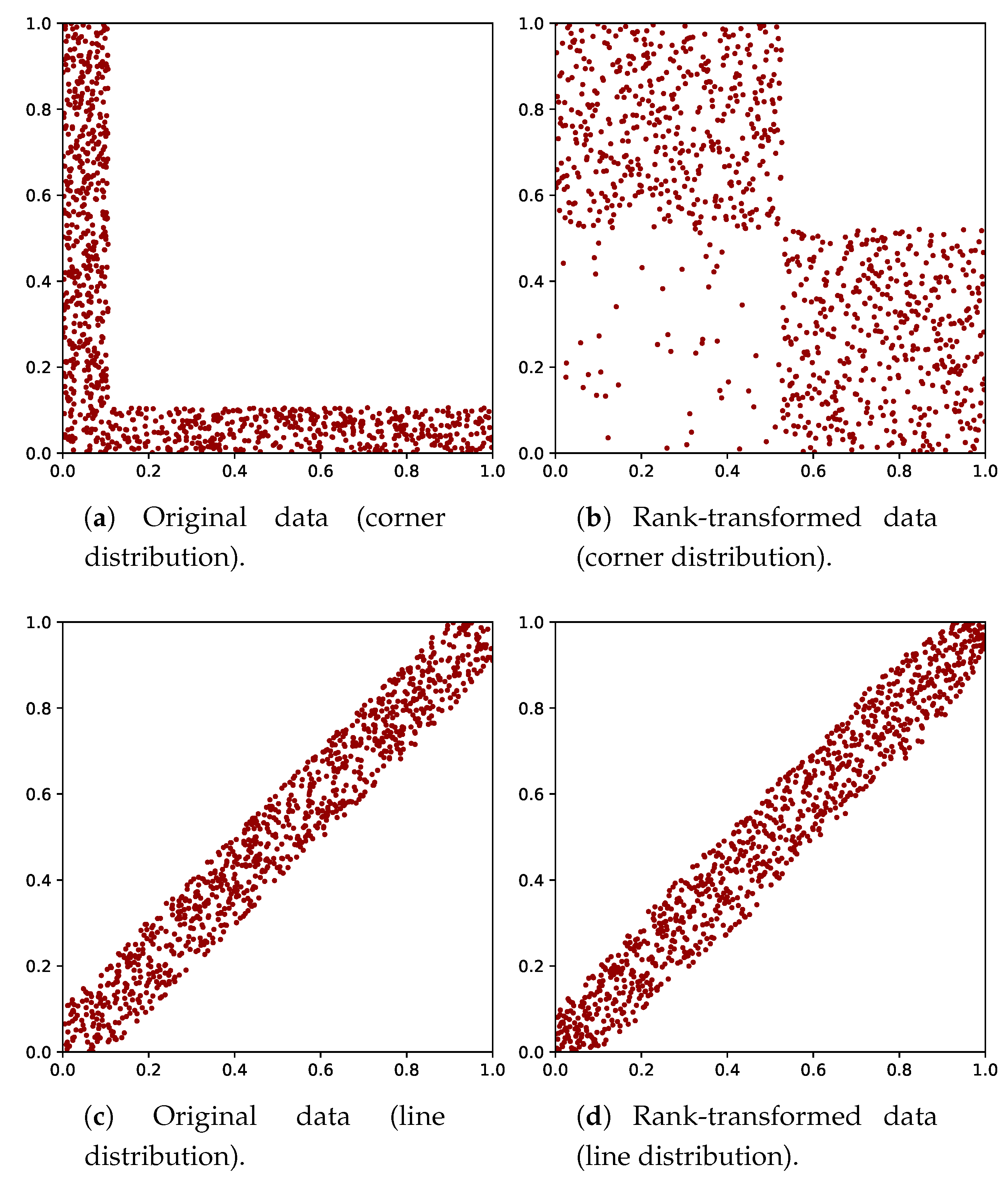
2.2. Entropy as Measure of Dependence
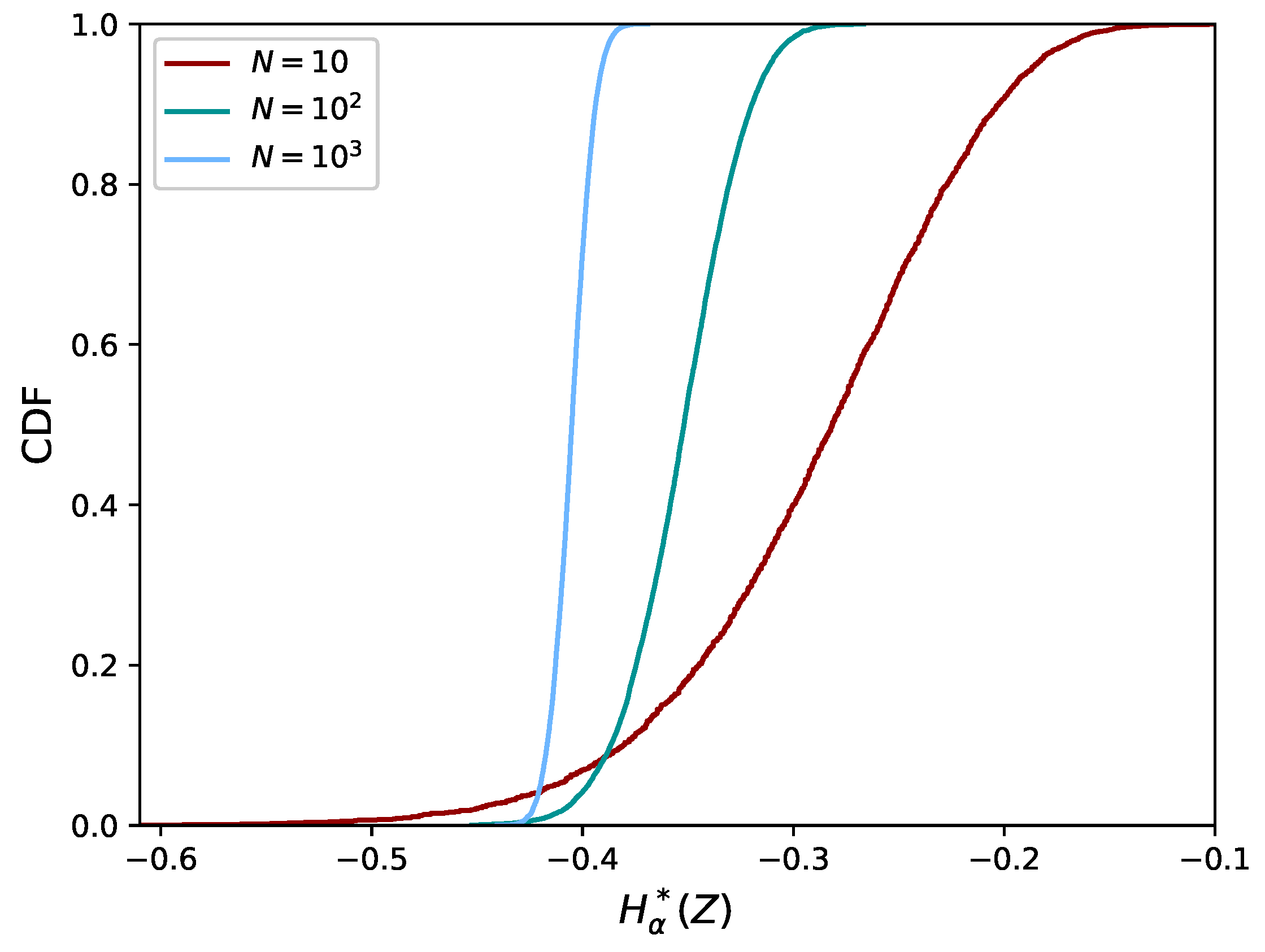
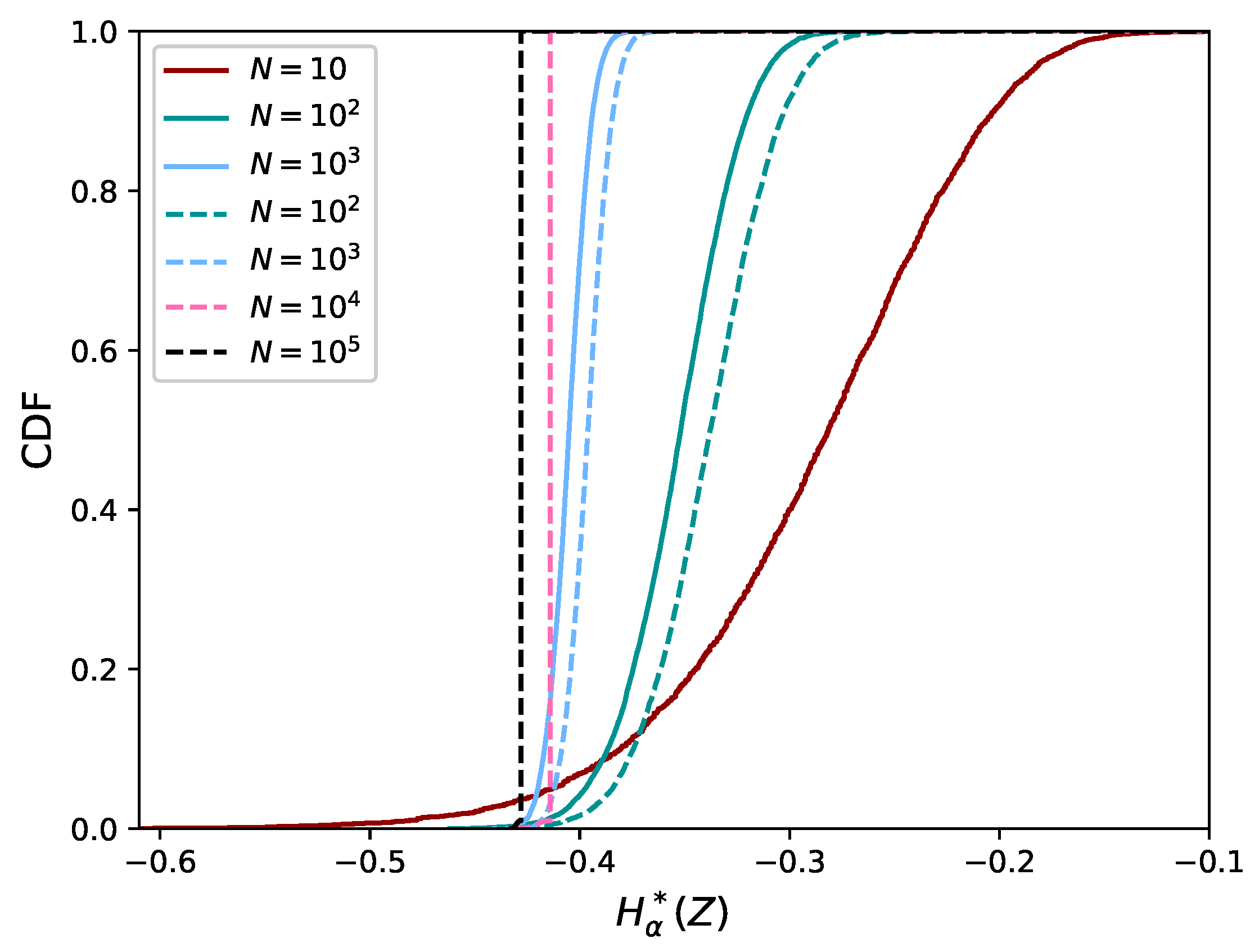
2.3. Estimator of the Rényi Entropy
2.4. Quantifier of Dependence
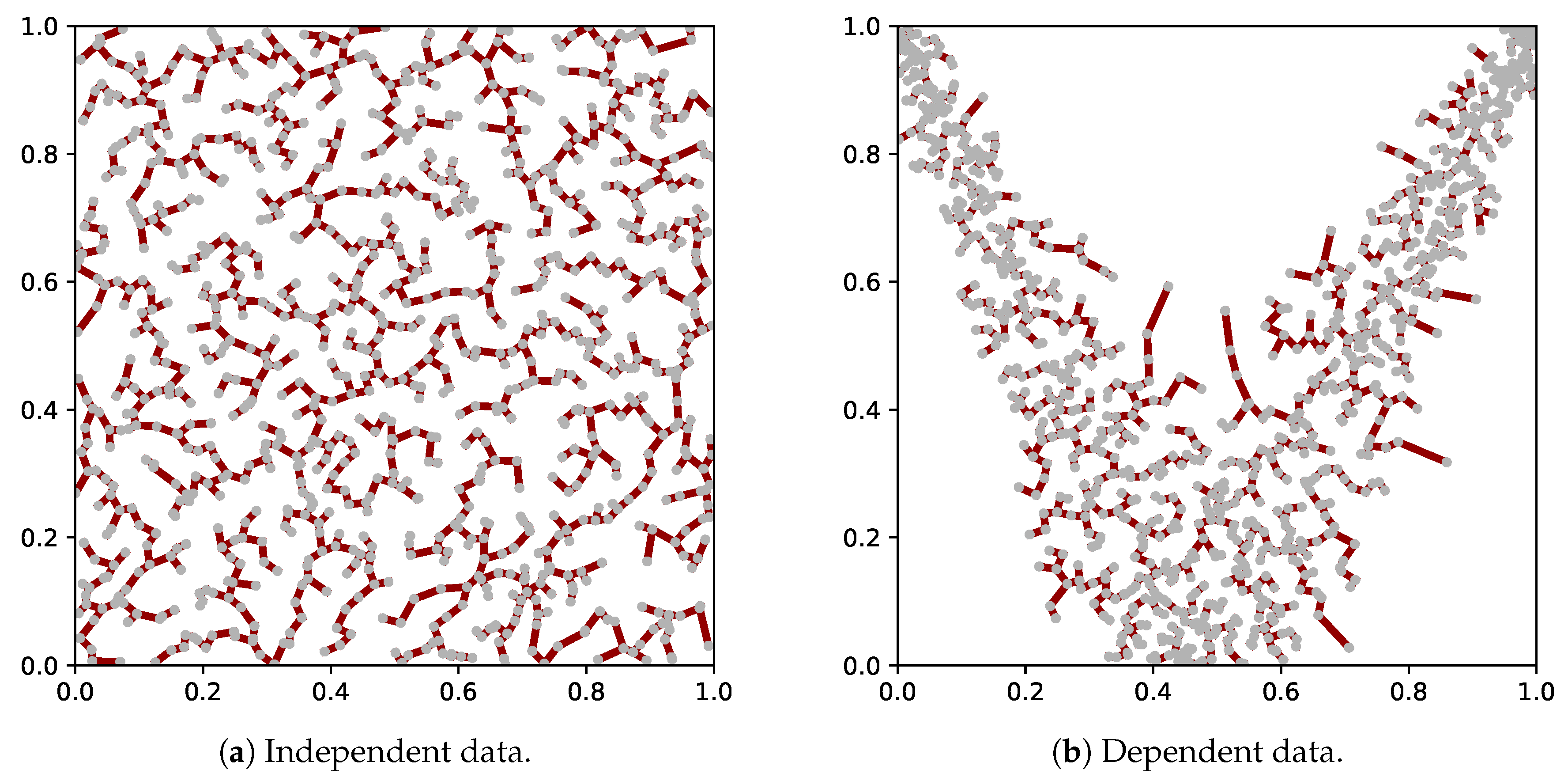
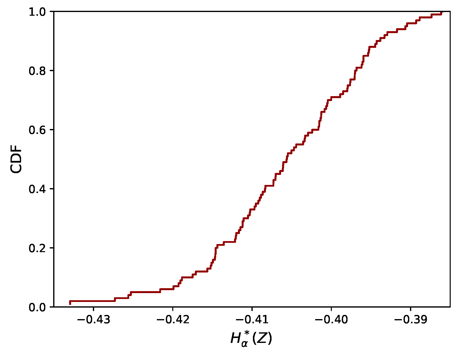
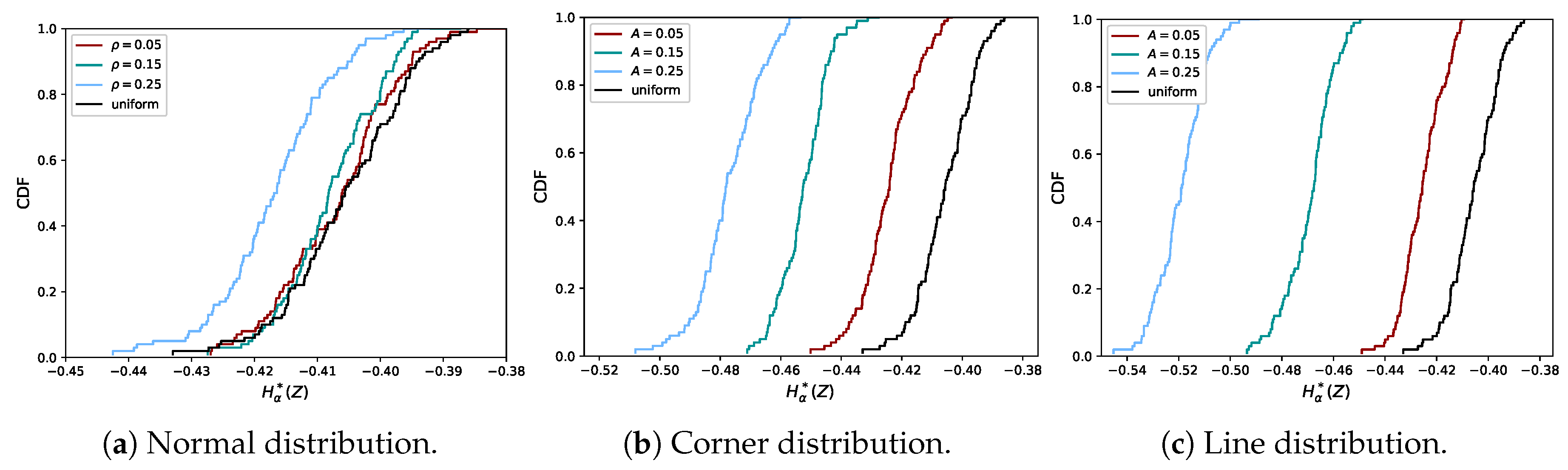
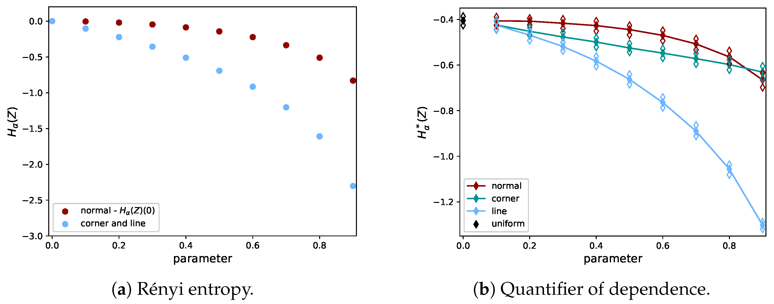
2.5. Proof of Concept
3. Approximation Methods
3.1. Sampling-Based MST
3.2. Cluster-Based MST
3.3. Multilevel MST
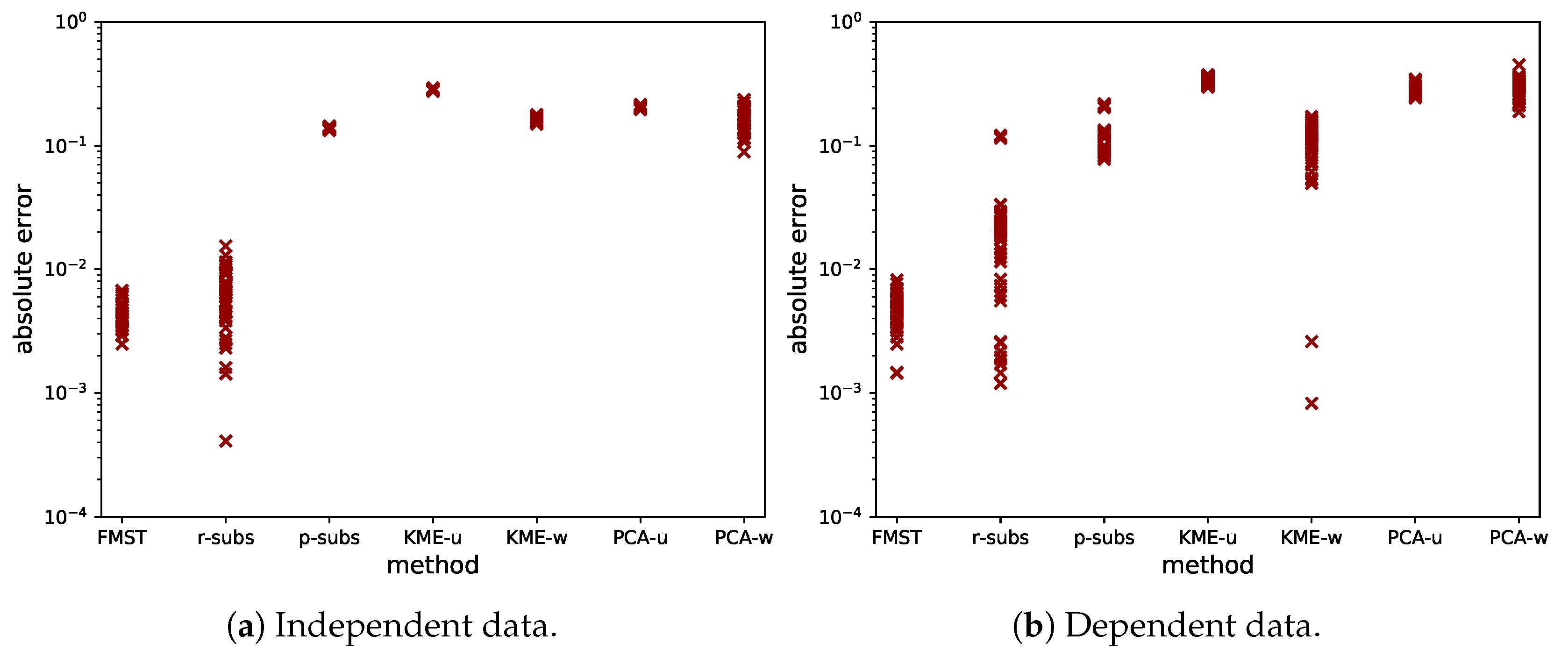
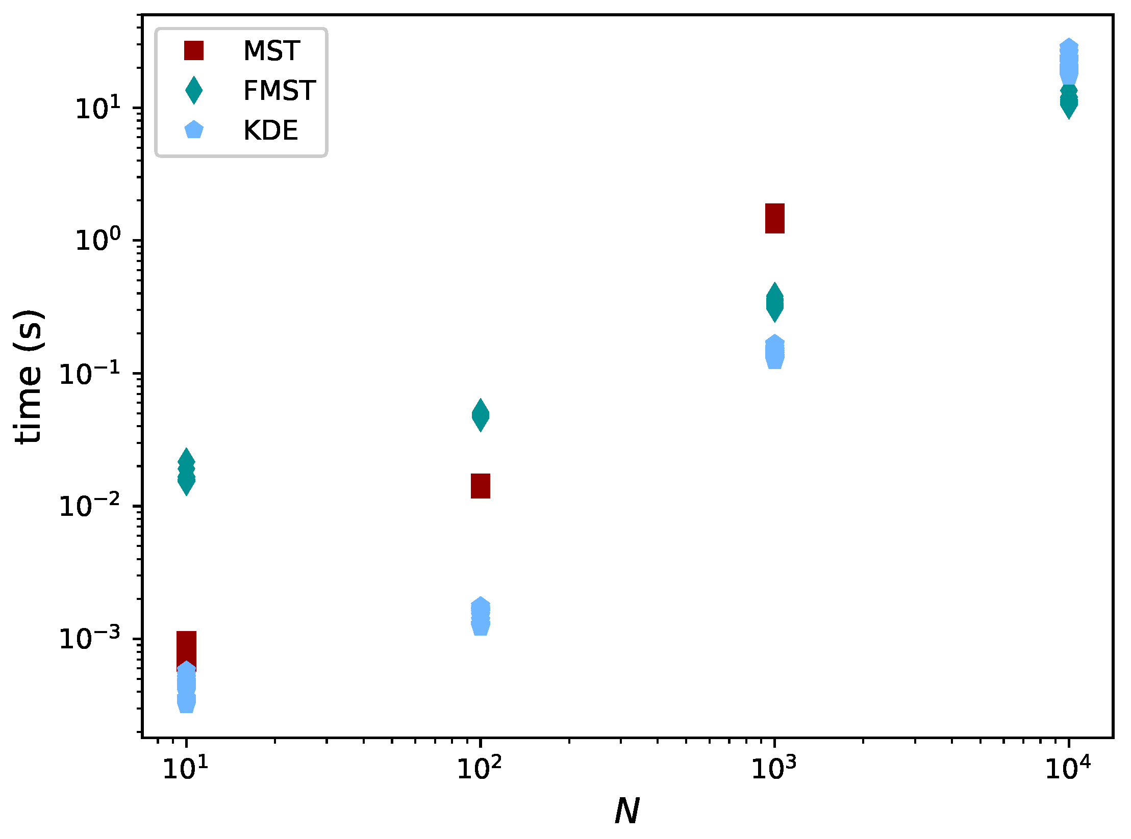
3.4. Comparison
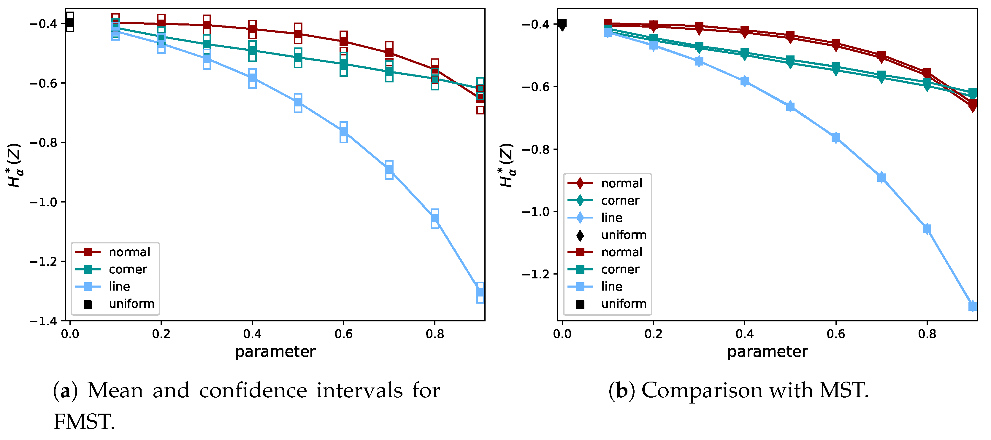
4. Validation of the Proposed FMST Estimator
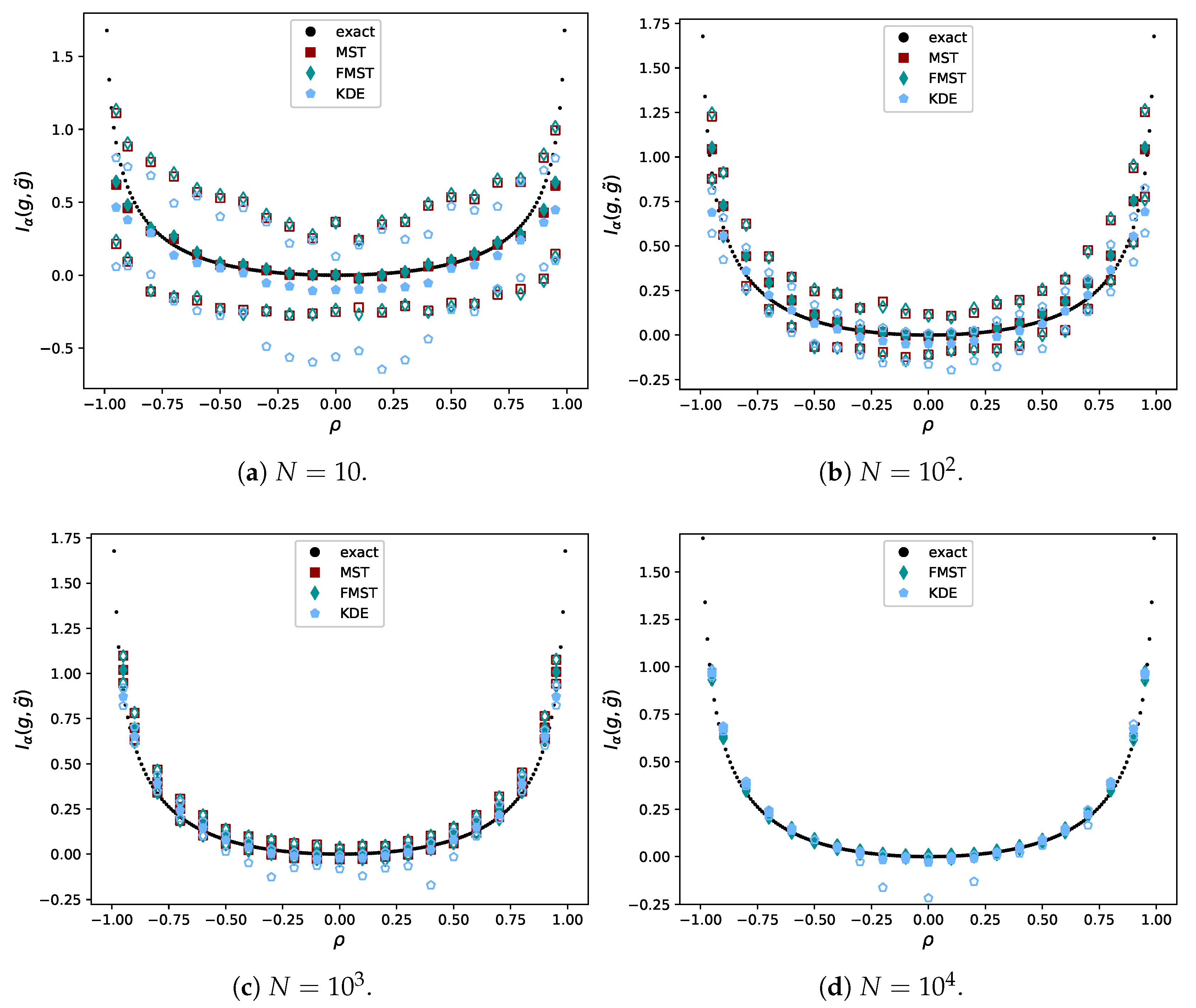
4.1. Comparison with the Exact Value of the Rényi Divergence
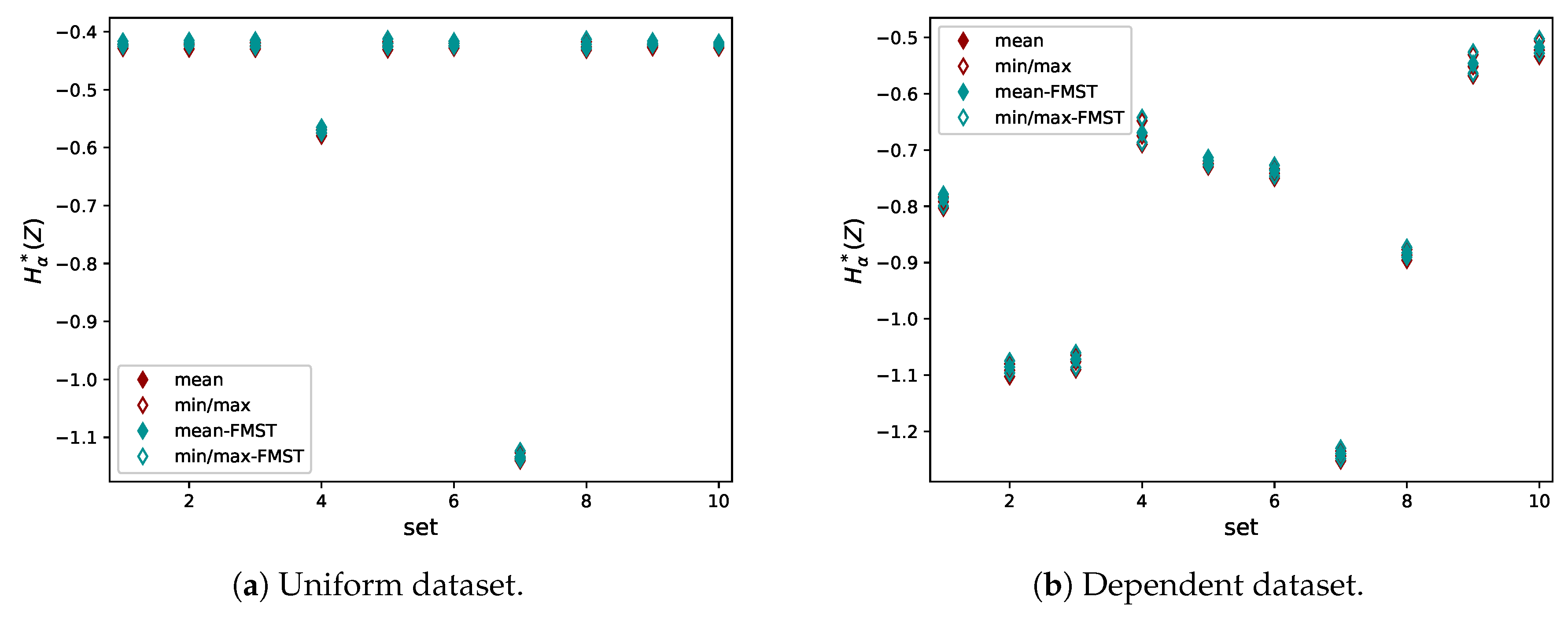
5. Test Cases
5.1. Ishigami Function
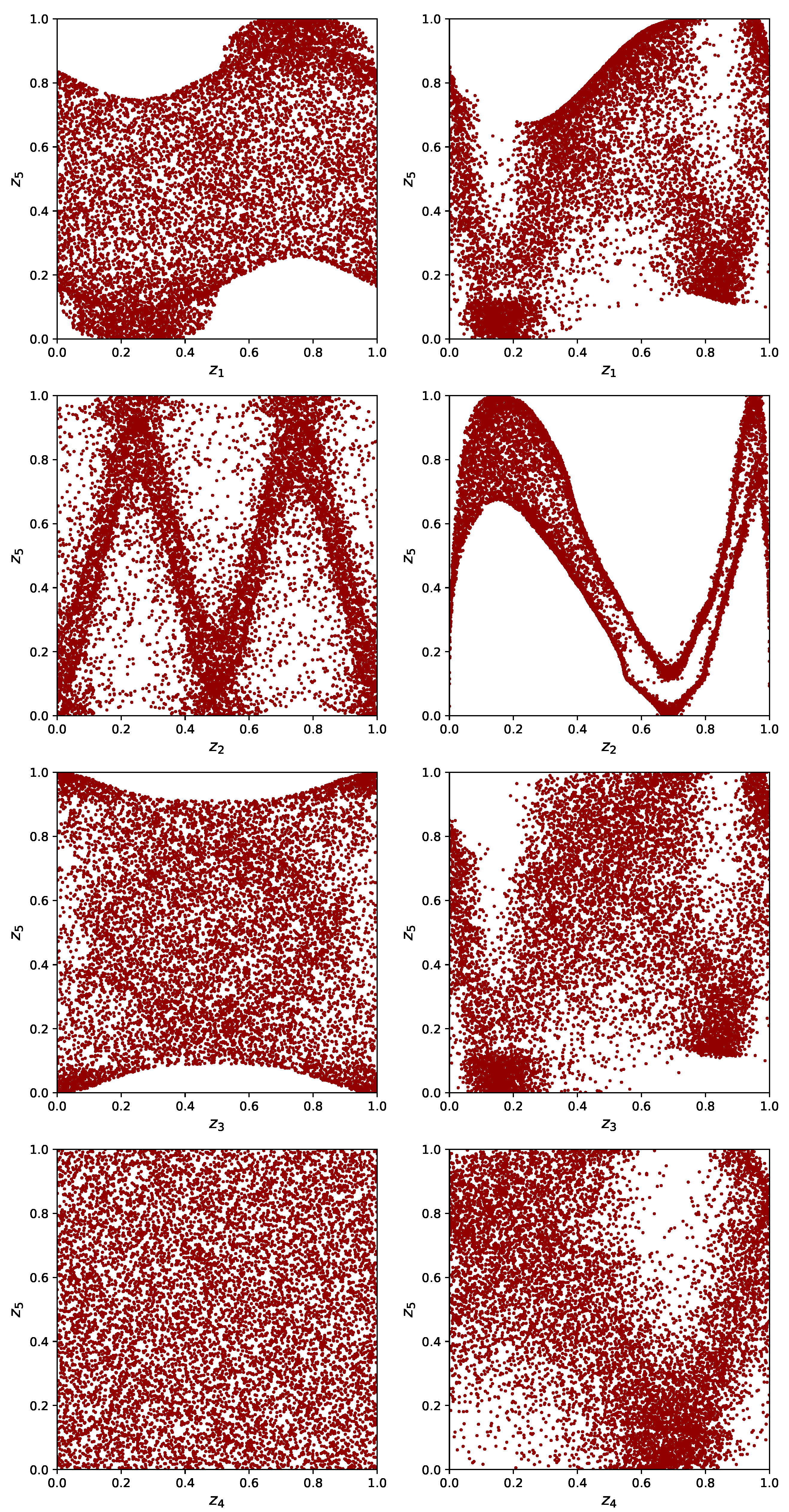
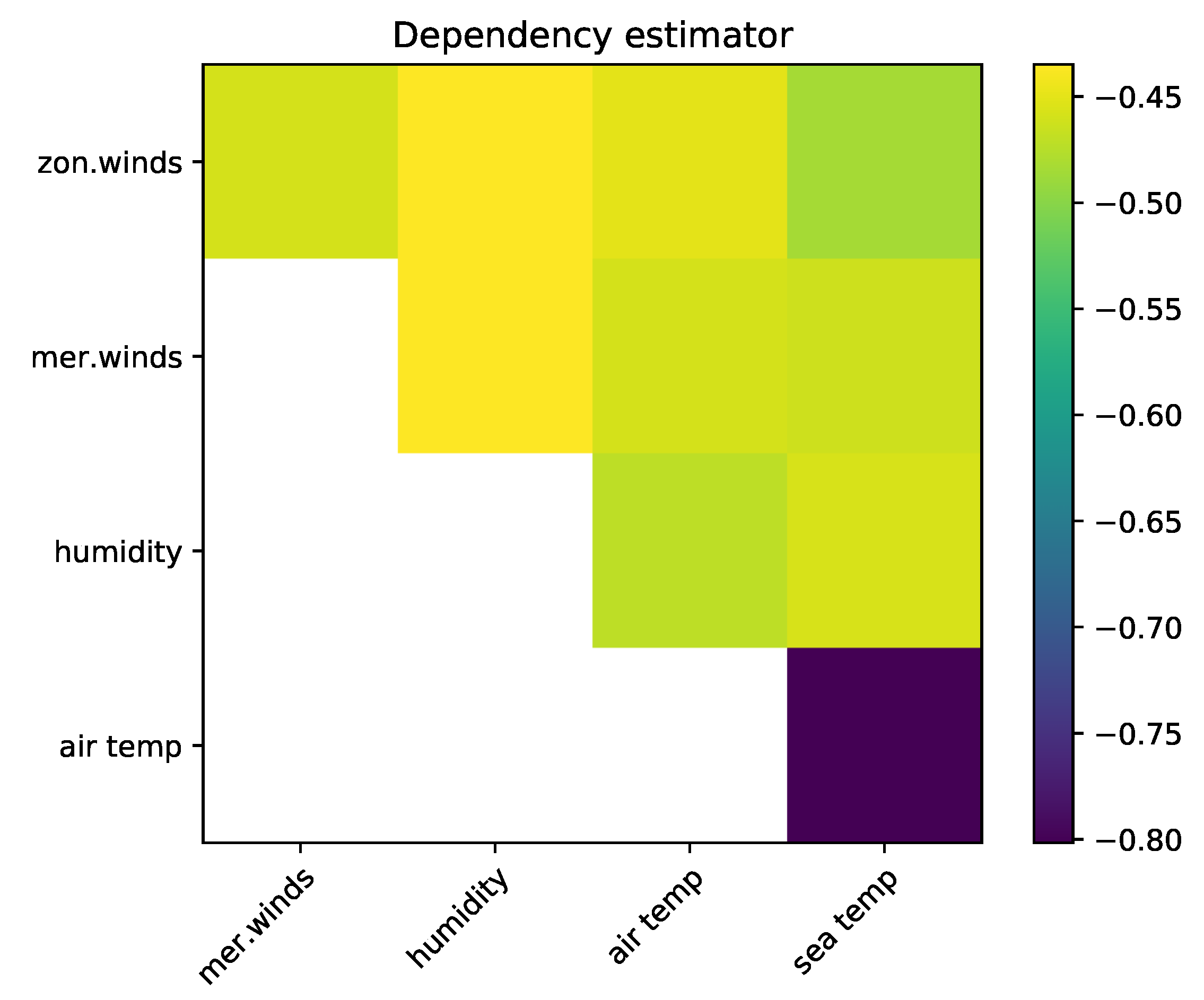
5.2. The El Niño Dataset
6. Discussion
Author Contributions
Funding
Conflicts of Interest
References
- Sullivan, T.J. Introduction to Uncertainty Quantification; Springer: Berlin, Germany, 2015; Volume 63. [Google Scholar]
- Ghanem, R.; Higdon, D.; Owhadi, H. Handbook of Uncertainty Quantification; Springer: Berlin, Germany, 2017. [Google Scholar]
- Le Maître, O.P.; Knio, O.M. Spectral Methods for Uncertainty Quantification: With Applications to Computational Fluid Dynamics; Scientific Computation; Springer: Berlin, Germany, 2010. [Google Scholar]
- Helton, J.C.; Johnson, J.D.; Sallaberry, C.J.; Storlie, C.B. Survey of sampling-based methods for uncertainty and sensitivity analysis. Reliab. Eng. Syst. Saf. 2006, 91, 1175–1209. [Google Scholar] [CrossRef]
- Saltelli, A.; Ratto, M.; Andres, T.; Campolongo, F.; Cariboni, J.; Gatelli, D.; Saisana, M.; Tarantola, S. Global Sensitivity Analysis: The Primer; John Wiley & Sons: Hoboken, NJ, USA, 2008. [Google Scholar]
- Iooss, B.; Lemaître, P. A Review on Global Sensitivity Analysis Methods. In Uncertainty Management in Simulation-Optimization of Complex Systems; Springer: Berlin, Germany, 2015; pp. 101–122. [Google Scholar]
- Cover, T.M.; Thomas, J.A. Elements of Information Theory, 2nd ed.; John Wiley & Sons: Hoboken, NJ, USA, 2006. [Google Scholar]
- Hero, A.O.; Ma, B.; Michel, O.J.J.; Gorman, J. Applications of Entropic Spanning Graphs. IEEE Signal Process. Mag. 2002, 19, 85–95. [Google Scholar] [CrossRef]
- Hero, A.O.; Costa, J.; Ma, B. Asymptotic Relations between Minimal Graphs and α-Entropy; Technical Report 334; Electrical Engineering and Computer Science—Communications and Signal Processing Laboratory, University of Michigan: Ann Arbor, MI, USA, 2003. [Google Scholar]
- Hero, A.O.; Michel, O.J.J. Robust Entropy Estimation Strategies Based on Edge Weighted Random Graphs. Proc. SPIE 1998, 3459, 250–261. [Google Scholar]
- Kruskal, J.B. On the shortest spanning subtree of a graph and the traveling salesman problem. Proc. Am. Math. Soc. 1956, 7, 48–50. [Google Scholar] [CrossRef]
- Prim, R.C. Shortest connection networks and some generalizations. Bell Labs Tech. J. 1957, 36, 1389–1401. [Google Scholar] [CrossRef]
- Auder, B.; Iooss, B. Global sensitivity analysis based on entropy. In Safety, Reliability and Risk Analysis, Proceedings of the ESREL 2008 Conference, Valencia, Spain, 22–25 September 2008; CRC Press: Boca Raton, FL, USA; pp. 2107–2115.
- Liu, H.; Chen, W.; Sudjianto, A. Relative Entropy Based Method for Probabilistic Sensitivity Analysis in Engineering Design. J. Mech. Des. 2006, 128, 326–336. [Google Scholar] [CrossRef]
- van Erven, T.; Harremoes, P. Rényi Divergence and Kullback-Leibler Divergence. IEEE Trans. Inf. Theory 2014, 60, 3797–3820. [Google Scholar] [CrossRef]
- Pál, D.; Póczos, B.; Szepesvári, C. Estimation of Rényi entropy and mutual information based on generalized nearest-neighbor graphs. In Proceedings of the 23rd International Conference on Neural Information Processing Systems, Vancouver, BC, Canada, 6–9 December 2010; pp. 1849–1857. [Google Scholar]
- Moon, K.; Sricharan, K.; Greenewald, K.; Hero, A. Ensemble Estimation of Information Divergence. Entropy 2018, 20, 560. [Google Scholar] [CrossRef]
- Hero, A.; Michel, O.J.J. Estimation of Rényi information divergence via pruned minimal spanning trees. In Proceedings of the IEEE Signal Processing Workshop on Higher-Order Statistics, Caesarea, Israel, 16 June 1999; pp. 264–268. [Google Scholar]
- Rosenblatt, M. Remarks on a multivariate transformation. Ann. Math. Stat. 1952, 23, 470–472. [Google Scholar] [CrossRef]
- Torre, E.; Marelli, S.; Embrechts, P.; Sudret, B. A general framework for data-driven uncertainty quantification under complex input dependencies using vine copulas. Probab. Eng. Mech. 2018. [Google Scholar] [CrossRef]
- Conover, W.J. The rank transformation—An easy and intuitive way to connect many nonparametric methods to their parametric counterparts for seamless teaching introductory statistics courses. Wiley Interdiscip. Rev. Comput. Stat. 2012, 4, 432–438. [Google Scholar] [CrossRef]
- Spearman, C. The proof and measurement of association between two things. Am. J. Psychol. 1904, 15, 72–101. [Google Scholar] [CrossRef]
- Csiszár, I.; Shields, P.C. Information theory and statistics: A tutorial. Found. Trends Commun. Inf. Theory 2004, 1, 417–528. [Google Scholar] [CrossRef]
- Hero, A.O.; Ma, B.; Michel, O.; Gorman, J. Alpha-Divergence for Classification, Indexing and Retrieval; Technical Report CSPL-328; Communication and Signal Processing Laboratory, University of Michigan: Ann Arbor, MI, USA, 2001. [Google Scholar]
- Silverman, B.W. Density Estimation for Statistics and Data Analysis; Chapman & Hall/CRC: Boca Raton, FL, USA, 1986. [Google Scholar]
- Noshad, M.; Moon, K.R.; Sekeh, S.Y.; Hero, A.O. Direct estimation of information divergence using nearest neighbor ratios. In Proceedings of the 2017 IEEE International Symposium on Information Theory (ISIT), Aachen, Germany, 25–30 June 2017; pp. 903–907. [Google Scholar]
- Zhong, C.; Malinen, M.; Miao, D.; Fränti, P. A fast minimum spanning tree algorithm based on K-means. Inf. Sci. 2015, 295, 1–17. [Google Scholar] [CrossRef]
- Celebi, M.E.; Kingravi, H.A.; Vela, P.A. A comparative study of efficient initialization methods for the K-means clustering algorithm. Expert Syst. Appl. 2013, 40, 200–210. [Google Scholar] [CrossRef]
- Steinhaus, H. Sur la division des corps matériels en parties. Bull. de l’Académie Polonaise des Sci. 1956, IV, 801–804. (In French) [Google Scholar]
- Eggels, A.W.; Crommelin, D.T.; Witteveen, J.A.S. Clustering-based collocation for uncertainty propagation with multivariate dependent inputs. Int. J. Uncertain. Quantif. 2018, 8. [Google Scholar] [CrossRef]
- Scott, J. Multivariate Density Estimation; Wiley Series in Probability and Statistics; John Wiley & Sons: Hoboken, NJ, USA, 1992. [Google Scholar]
- Ishigami, T.; Homma, T. An Importance Quantification Technique in Uncertainty Analysis for Computer Models. In Proceedings of the First International Symposium on Uncertainty Modeling and Analysis, College Park, MD, USA, 3–5 December 1990; pp. 398–403. [Google Scholar]
- Sobol’, I.M. Global sensitivity indices for nonlinear mathematical models and their Monte Carlo estimates. Math. Comput. Simul. 2001, 55, 271–280. [Google Scholar] [CrossRef]
- Crestaux, T.; Le Maître, O.; Martinez, J.M. Polynomial chaos expansion for sensitivity analysis. Reliab. Eng. Syst. Saf. 2009, 94, 1161–1172. [Google Scholar] [CrossRef]
- Dheeru, D.; Karra Taniskidou, E. UCI Machine Learning Repository. 2017. Available online: http://archive.ics.uci.edu/ml (accessed on 22 October 2018).
- Pfahl, S.; Niedermann, N. Daily covariations in near-surface relative humidity and temperature over the ocean. J. Geophys. Res. 2011, 116. [Google Scholar] [CrossRef]


| 0.314 | 0.558 | −0.570 | |
| 0.442 | 0.442 | −1.133 | |
| 0 | 0.244 | −0.420 | |
| 0 | 0 | −0.421 |
© 2019 by the authors. Licensee MDPI, Basel, Switzerland. This article is an open access article distributed under the terms and conditions of the Creative Commons Attribution (CC BY) license (http://creativecommons.org/licenses/by/4.0/).
Share and Cite
Eggels, A.; Crommelin, D. Quantifying Data Dependencies with Rényi Mutual Information and Minimum Spanning Trees. Entropy 2019, 21, 100. https://doi.org/10.3390/e21020100
Eggels A, Crommelin D. Quantifying Data Dependencies with Rényi Mutual Information and Minimum Spanning Trees. Entropy. 2019; 21(2):100. https://doi.org/10.3390/e21020100
Chicago/Turabian StyleEggels, Anne, and Daan Crommelin. 2019. "Quantifying Data Dependencies with Rényi Mutual Information and Minimum Spanning Trees" Entropy 21, no. 2: 100. https://doi.org/10.3390/e21020100
APA StyleEggels, A., & Crommelin, D. (2019). Quantifying Data Dependencies with Rényi Mutual Information and Minimum Spanning Trees. Entropy, 21(2), 100. https://doi.org/10.3390/e21020100