On Achievable Distortion in Sending Gaussian Sources over a Bandwidth-Matched Gaussian MAC with No Transmitter CSI


Abstract
1. Introduction
1.1. Related Work
1.2. Main Contributions
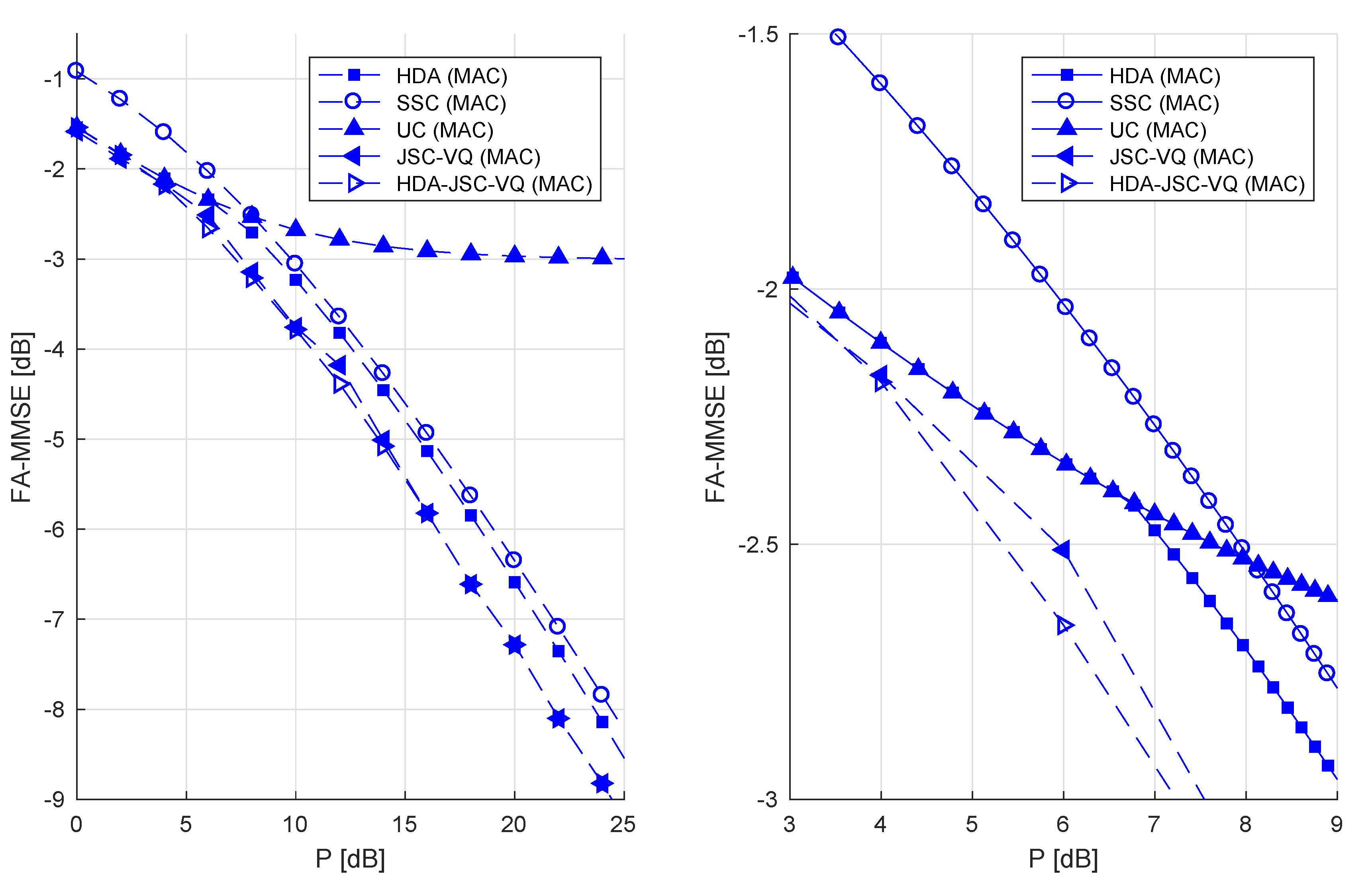
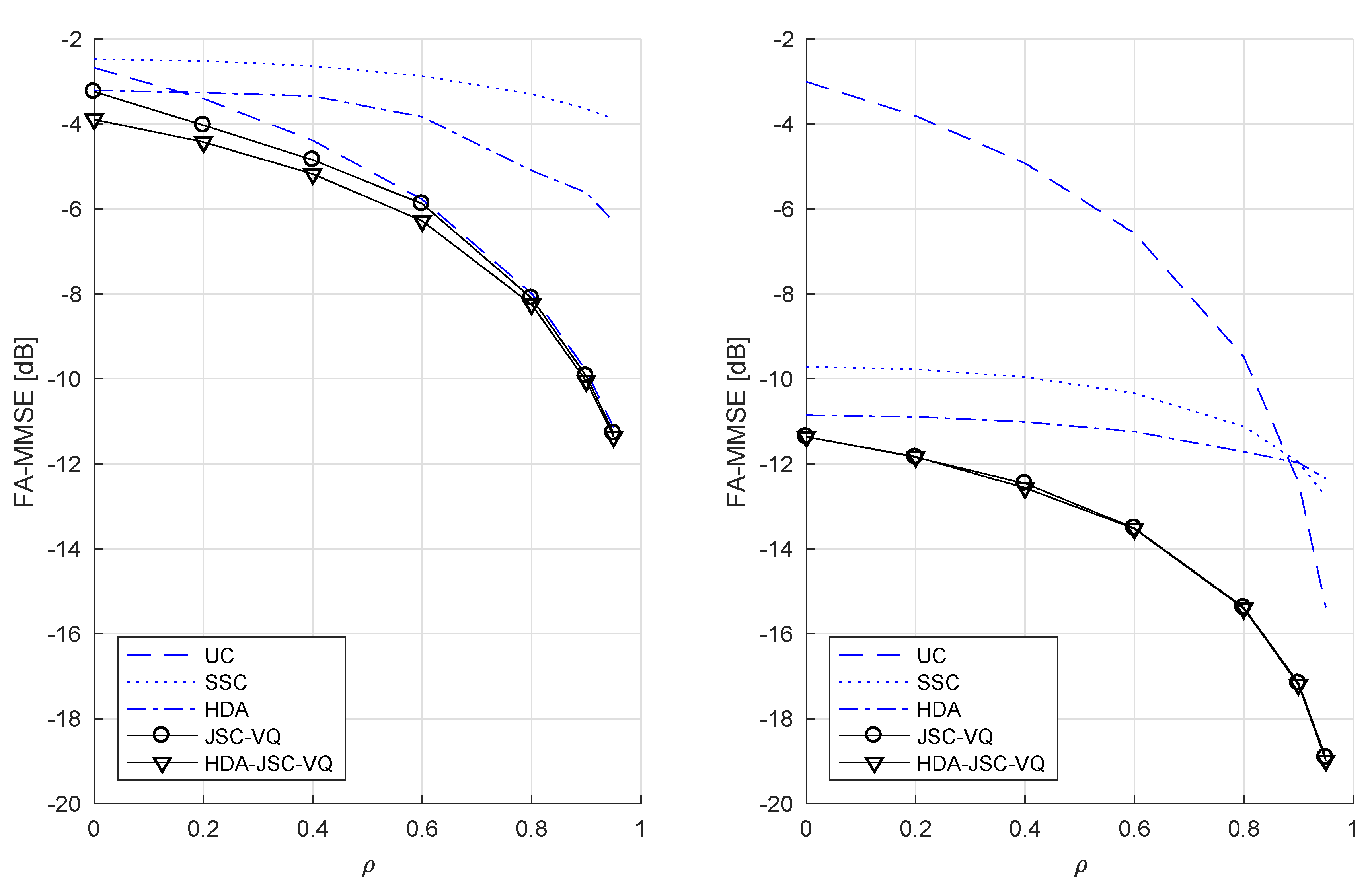
- The obvious and relatively straightforward to-determine upper-bounds to the DPF are the FA-MMSEs, which are achievable with uncoded transmission and SSC coding. In this paper, we derive an alternative bound by considering conventional hybrid digital–analog (HDA) coding, wherein vector quantization error in conventional digital coding is transmitted in analog form by superposition. As expected, the numerical results show that, for uncorrelated sources, HDA coding improves on both SSC coding and uncoded transmission. For correlated sources, uncoded transmission has an advantage over HDA coding at low CSNRs where digital coding frequently suffers receiver outages due to lack of CSI at the the transmitters.
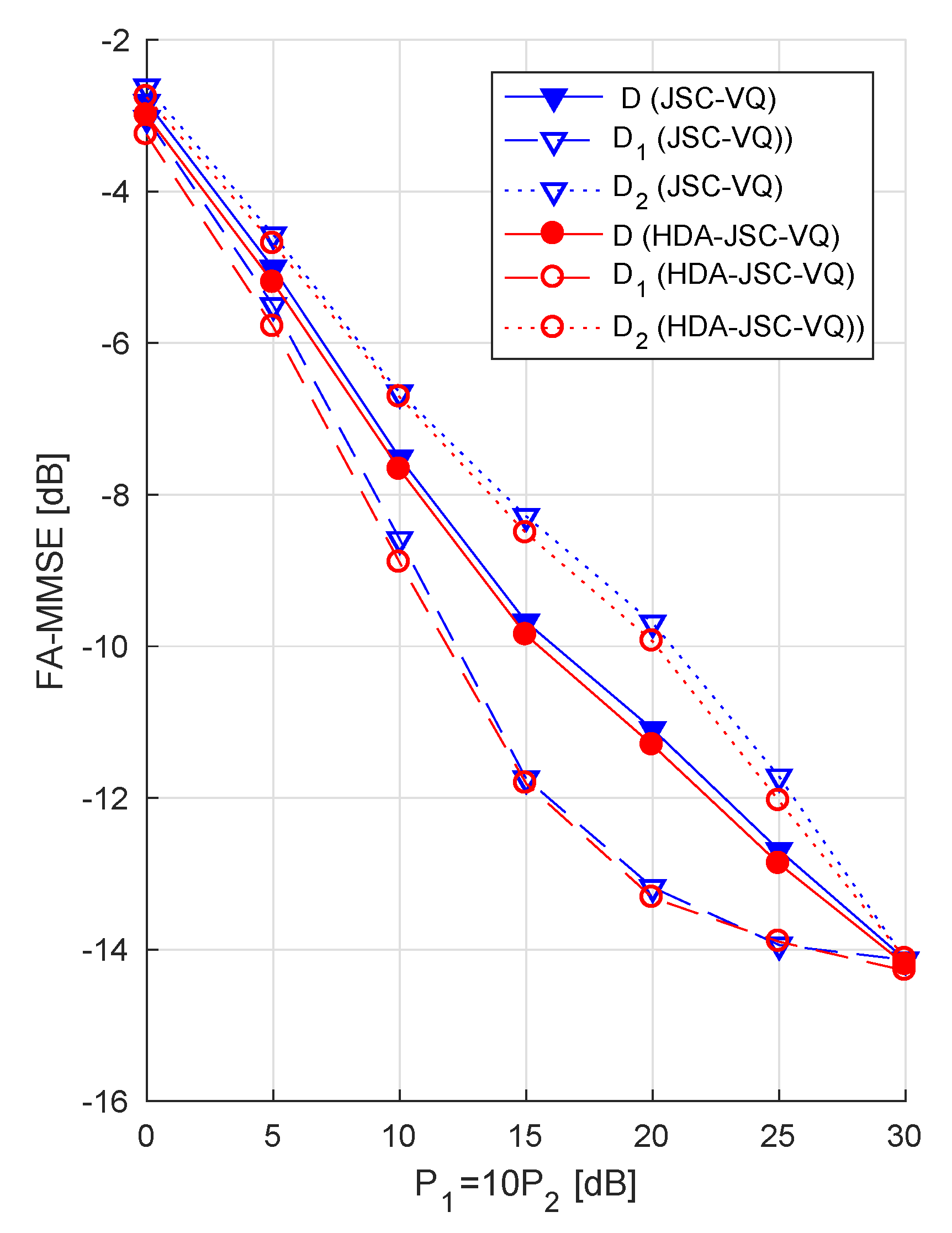
- It is shown in [10] that when the sources are correlated and the GMAC is fixed (no fading), although uncoded transmission of the sources over the GMAC is optimal at SNRs below a threshold determine by the source correlation, the uncoded transmission of vector quantized sources directly over the GMAC (JSC-VQ) is asymptotically (as the CSNR approaches infinity) optimal. Furthermore, it has been shown that this scheme, when enhanced with a superimposed uncoded transmission of the sources (HDA-JSC-VQ), is nearly optimal at all CSNRs. Based on these observations, we derive two upper bounds to the DPF for the fading GMAC, referred as the JSC-VQ bound and HDA-JSC-VQ bound, respectively. Although these bound do not have expressions that can be readily interpreted, they can be numerically computed. It is observed that JSC-VQ and HDA-JSC-VQ bounds are not significantly different, regardless of the source correlation. However, the comparison of these bounds with the distortion bound for SSC coding shows a gap that grows with source correlation and CSNR. Although there exists a gap even when the sources are uncorrelated, this gap is relatively much smaller. The HDA-JSC-VQ bound established here is the lowest known upper bound to unknown DPF. It is shown that, for highly correlated sources and under low average CSNRs, uncoded transmission can achieve performance approaching the HDA-JSC-VQ bound.
2. Problem Definition
Notation and Terminology
3. Separate Source-Channel Coding
3.1. Uncorrelated Sources
3.2. Correlated Sources
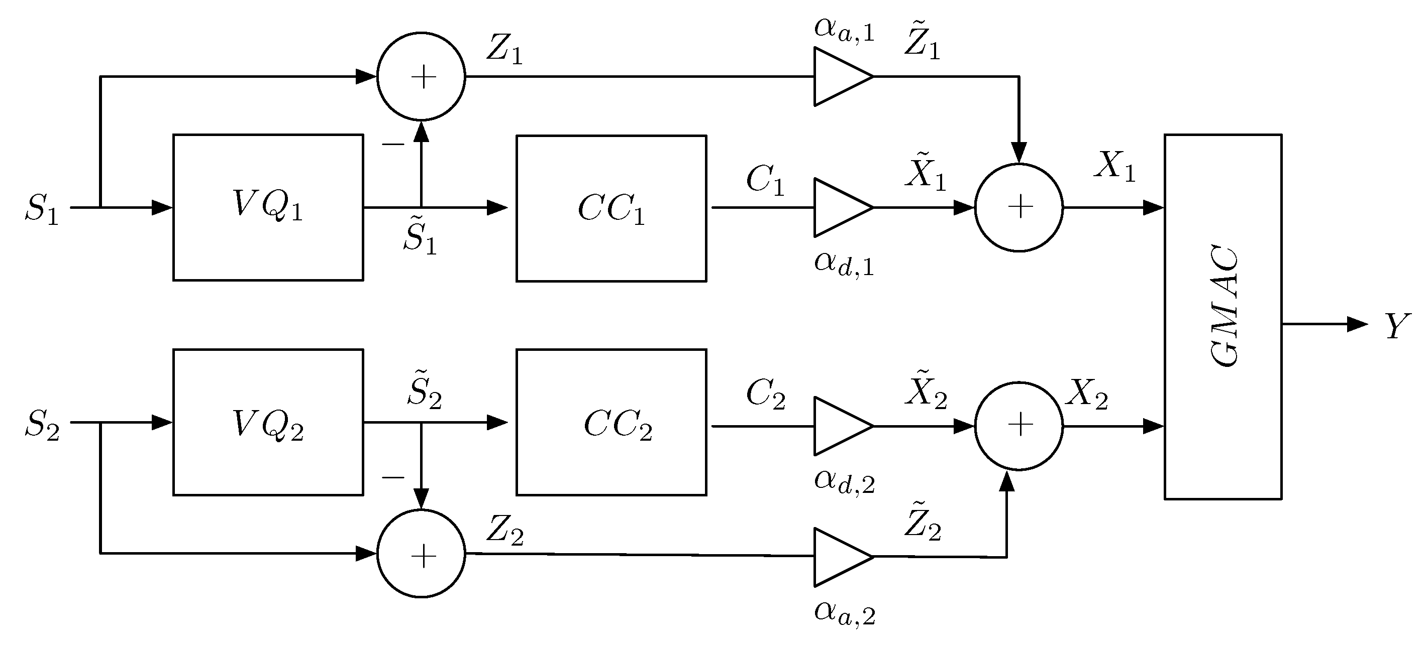
4. Conventional HDA Coding
- Partial outage event (either or is decodable, but not both): is decodable while is not decodable if and only if
- Total outage event : Neither nor is decodable if and only if Equation (11) is violated for and Equation (12) is violated.
4.1. No Outage Event ()
- 1.
- For the special case of uncoded transmission, we can set and ().
- 2.
- On the other hand, by setting , we obtain the achievable MMSE of a purely digital SSC coding system. However, for correlated sources, this MMSE is less than that given by the Lemma 1. This is because the digital encoder in Figure 1 does not achieve a distributed coding gain, as does the digital encoder in Section 3. To achieve a coding gain, a distributed VQ must be used, but this will render the quantization errors of the two source uncorrelated, preventing us from exploiting the correlation between the GMAC inputs to our advantage. The advantage of the HDA scheme in Figure 1 is its robustness against unknown CSI. In particular, when the two sources are correlated, so will be their quantization errors. This correlation allows for a form of statistical cooperation at the GMAC output as reflected by the appearance of in Equation (16), see Appendix C.
4.2. Partial Outage Event ()
4.3. Total Outage Event ()
5. JSC Coding
5.1. JSC-VQ
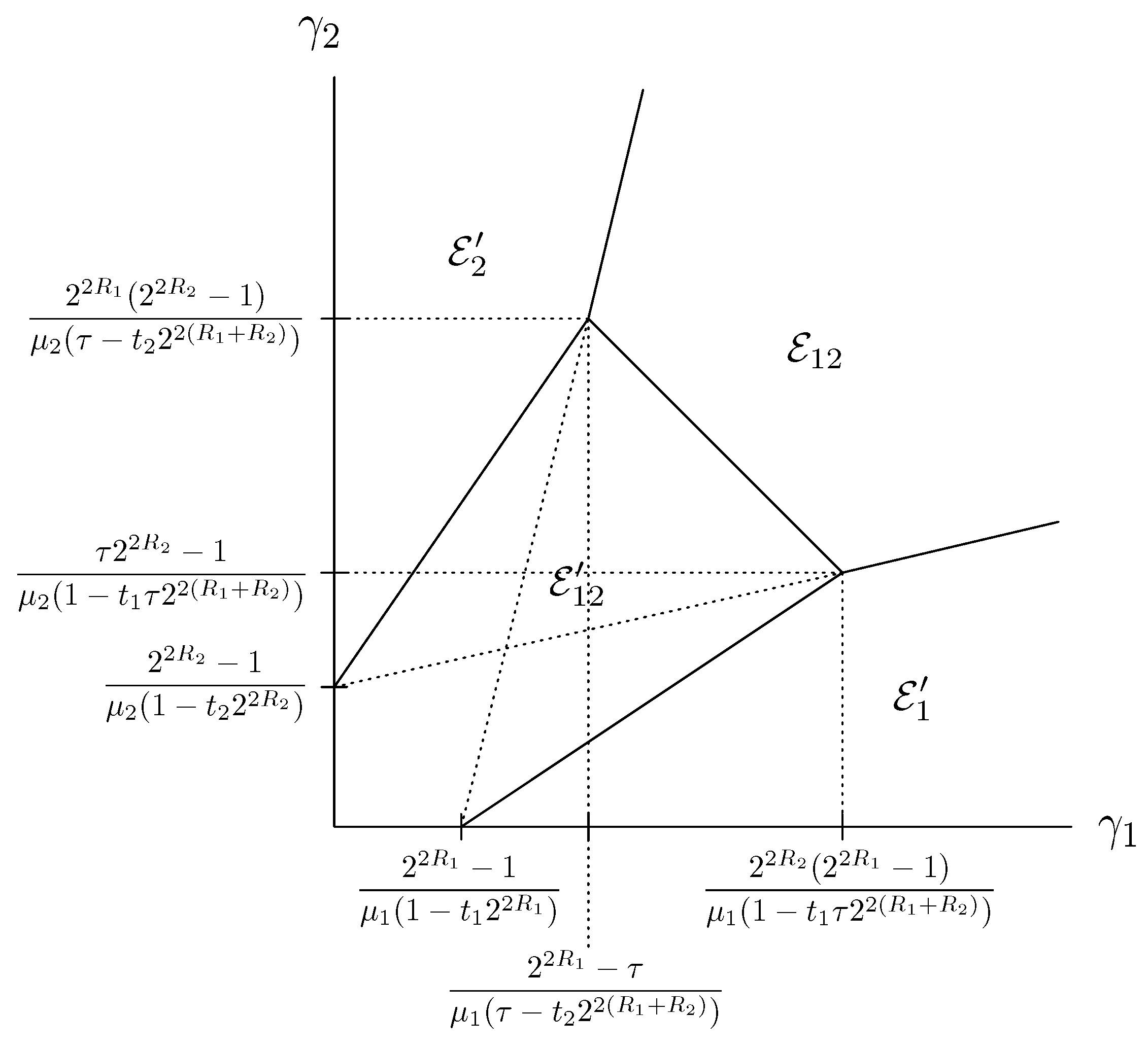
- No-outage event : The set of all rate pairs for which occurs are given by the following lemma.Lemma 2.For given , , , and ρ, both of the source-channel VQ codewords can be detected with an asymptotically vanishing error probability, if satisfywhere is given by Equation (9).Proof .Denote all pairs that satisfy the above constraints by . Let the codeword pair found in the detection step be . If then and . In this case, the linear estimator need not use the channel output (), and the source sequences can be reconstructed asSee Appendix D. □The MMSE of the linear estimator for is given by Equation (A24).
- Partial outage event : The set of all rate pairs for which () occurs are given by the following lemma.Theorem 1.For given , , , and ρ, the codeword is decodable and is undecodable if and only iffor .Proof .Denote all pairs which satisfy above constraints by . If , then and . The source sequences are reconstructed asThe proof, considering the case and , is given in Appendix D. □The expressions for the MMSE of the linear estimator for are given by Equations (A25) and (A26).
- Total outage event : The set of all rate pairs for which occurs is given by the following lemma.Lemma 3.For given , , , and ρ, neither codeword can be decoded ifProof .Denote all pairs which satisfy above constraints by . The source sequences are reconstructed asFollows from Equations (24) and (25) in the previous two lemmas. □The expressions for the MMSE of the linear estimator for are given Equation (A27).
5.2. HDA-JSC-VQ Coding
- No-outage event : For fixed , the bounds on VQ rates required to guarantee error-free decoding of can be found through a slight generalization of the results in ([10], Theorem IV.6) to account for channel-gains and complex-valued random variables. In particular we can prove the following lemma. For satisfying the bounds in Lemma 4, the minimum achievable MMSE is given by Equation (A28).
- Partial outage event : Rate pairs for which only one codeword can be decoded is given by the following lemma.Lemma 5.For satisfying the bounds in Lemma 5, the minimum achievable MMSE is given by Equation (A29).For given , , , , and ρ, the necessary and sufficient conditions where only codeword , but not , is correctly decodable are
- Total outage event : Rate pairs for which neither codeword can be decoded is given by the following lemma.Lemma 6.For satisfying the bounds in Lemma 6, the minimum achievable MMSE is given by Equation (A30).For given , , , , and ρ, neither nor can be decoded if
6. Comparison of Bounds and Discussion
Author Contributions
Funding
Conflicts of Interest
Appendix A. Outage Probabilities in SSC Coding of Gaussian Sources
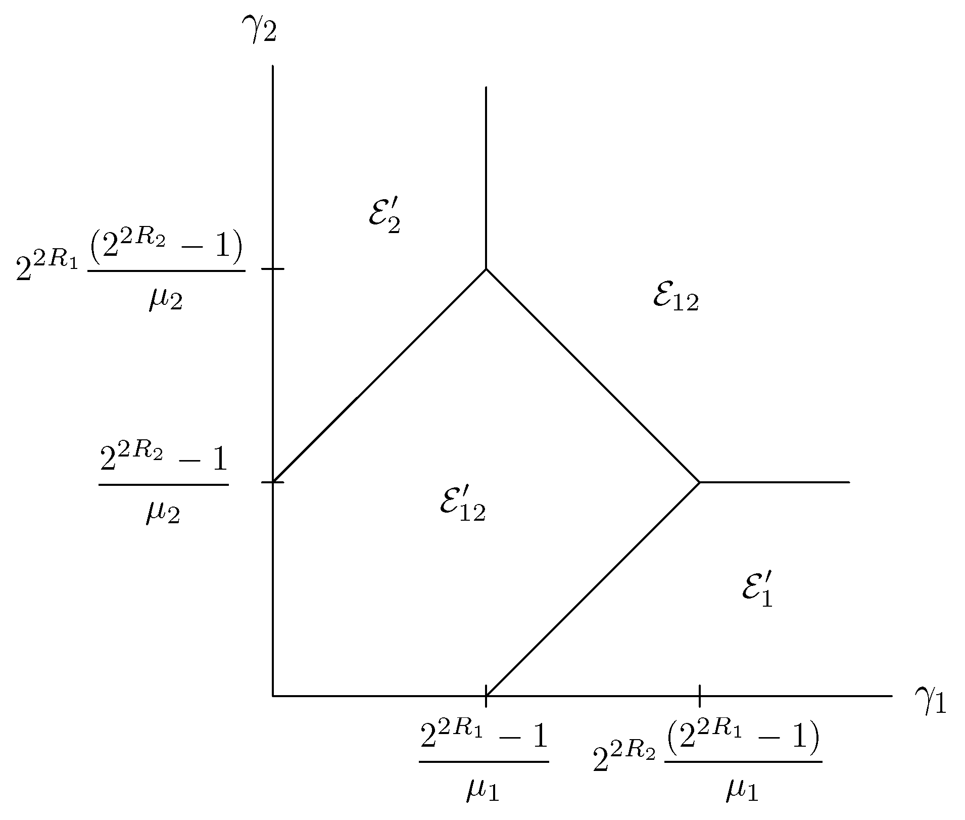
- (both codewords decodable):
- (only one codeword decodable):
- (neither codeword decodable):

Appendix B. Proof of Lemma 1
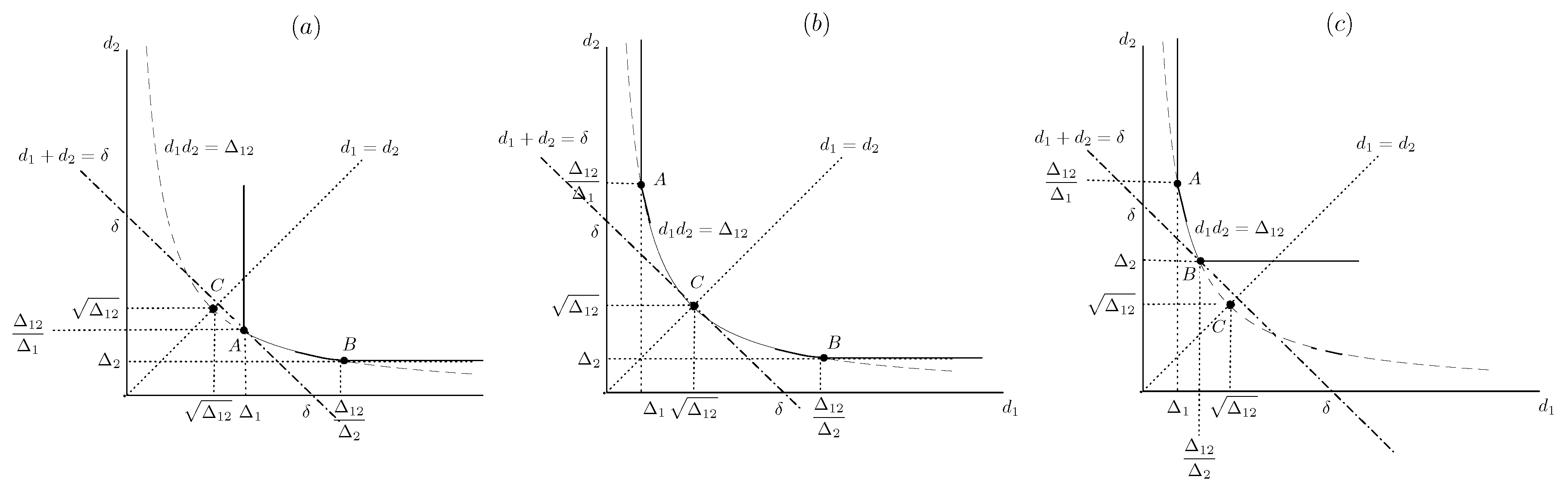
| A [Figure A2a], |
| B [Figure A2c], |
| C [Figure A2b]. |

Appendix C. Optimal Linear Estimators for HDA Coding
- No-outage event (): Linear estimator used in the HDA system, estimates the source sample , using the observation vector . Define the asymptotic autocovariance matrix and the cross-covariance vector . For optimal VQ of Gaussian sources, Equations (5)–(8) hold and the following can be verified.Let the optimal linear estimator coefficients be . Then, we have , .
- Partial outage event (): In this case, define , , and , which is a matrix whose elements areLet optimal linear estimates for and , be and . Then, we have and , where and with
- Total outage event (): The optimal source estimates are given by , for , where and
Appendix D. Proof of Lemma 2 and Theorem 1
Appendix D.1. Proof of Lemma 2
Appendix D.2. Proof of Theorem 1
- (i)
- what is the largest for which the joint decoding procedure described above can guarantee that as regardless of ?
- (ii)
- if is provided to the decoder, what is lowest above which the correct decoding of cannot be guaranteed?
- Statement A:
- For every it holds thatwhere only depends on , and z.First, by rewriting the LHS of Equation (A14), we haveNext, by rewriting LHS of the above inequality Equation (A15),Figure A3 illustrates an example of vectors and in the complex vector space . Let angles , and are defined as , and . The respective cosine values of and are given byRecalling that , for , , and (see Lemma A5), it can be shown thatBy substituting Equations (A16) and (A18) in Equation (A17), we can writeFigure A3. The definition of asymptotic angles used to prove Lemma A4.
 For choose such that , then it follows thatWith , theequality holds true when vectors , and are on the same plane. Note that and , it follows thatAs let , where is only a function of and N. Now Equation (A19) can be written asBy revisiting the definition of and , Equation (A20) can be rewritten asRecalling that , (A21) can be written asAS , , we can bound the real component of the inner product between the received signal vector and as follows,
 - Statement B:
- For every , we have the straightforward relationwhere is only a function of , and .
- Statement C:
- For every , it follows from the power constraint that
- Statement D:
- For every , the following implication holdswhereThis statement follows from rewriting the asand then lower bounding using Statement A and upper bounding and using Statements B and C, respectively.

Appendix E. MMSE of Linear Estimation Step in JSC-VQ and HDA-JSC-VQ Decoders
Appendix E.1. JSC-VQ System
- Outage event : Define the column vector whose covariance matrix isand let . The optimal linear estimator is whose coefficients are given by . The MMSE of this estimator is
- Partial outage event : Define the column vector whose covariance matrix isand let . The optimal linear estimator is whose coefficients are given by . The MMSE of this estimator is
- Partial outage event : Define the column vector whose covariance matrix isand let . The optimal linear estimator is whose coefficients are given by . The MMSE of this estimator is
- Total outage event : The optimal linear estimator is , where and the MMSE is
Appendix E.2. HDA-JSC-VQ System
- Outage event : Both and are decoded correctly. Unlike in the JSC-VQ system, the linear estimator is and the optimal coefficients are given by , where , and is the matrix whose -elements is . and . The MMSE is thus
- Partial outage event : Only is decoded correctly and hence
- Partial outage event : Only is decoded correctly and hence
- Total outage event : Neither nor is decoded correctly, and therefore
References
- Chong, C.Y.; Kumar, S.P. Sensor networks: Evolution, opportunities, and challenges. Proc. IEEE 2003, 91, 1247–1256. [Google Scholar] [CrossRef]
- Gastpar, M.; Vetterli, M. Source-channel communication in sensor networks. In Information Processing in Sensor Networks; Springer: Berlin/Heidelberg, Germany, 2003; pp. 162–176. [Google Scholar]
- Goldsmith, A.J.; Varaiya, P. Capacity of fading channels with channel side information. IEEE Trans. Inf. Theory 1997, 43, 1986–1992. [Google Scholar] [CrossRef]
- Cover, T.M.; Thomas, J.A. Elements of Information Theory, 2nd ed.; John Wiley: Hoboken, NJ, USA, 2006. [Google Scholar]
- Cover, T.M.; Gamal, A.E.; Salehi, M. Multiple access channels with arbitrarily correlated sources. IEEE Trans. Inf. Theory 1980, 26, 648–657. [Google Scholar] [CrossRef]
- Xiao, J.J.; Luo, Z.Q. Multiterminal Source–Channel Communication Over an Orthogonal Multiple-Access Channel. IEEE Trans. Inf. Theory 2007, 53, 3255–3264. [Google Scholar] [CrossRef]
- Tian, C.; Chen, J.; Diggavi, S.H.; Shitz, S.S. Optimality and Approximate Optimality of Source-Channel Separation in Networks. IEEE Trans. Inf. Theory 2014, 60, 904–917. [Google Scholar] [CrossRef]
- Wagner, A.B.; Tavildar, S.; Viswanath, P. Rate region of the quadratic Gaussian two-encoder source-coding problem. IEEE Trans. Inf. Theory 2008, 54, 1938–1961. [Google Scholar] [CrossRef]
- Ray, S.; Médard, M.; Effros, M.; Koetter, R. On Separation for multiple-access channels. In Proceedings of the 2006 IEEE Information Theory Workshop—ITW ’06, Punta del Este, Uruguay, 22–26 October 2006; pp. 399–403. [Google Scholar]
- Lapidoth, A.; Tinguely, S. Sending a bi-variate Gaussian source over a Gaussian MAC. IEEE Trans. Inf. Theory 2010, 56, 2714–2752. [Google Scholar] [CrossRef]
- Viswanathan, H.; Berger, T. The quadratic Gaussian CEO problem. IEEE Trans. Inf. Theory 1997, 43, 1549–1559. [Google Scholar] [CrossRef]
- Gastpar, M. Uncoded transmission is exactly optimal for a simple Gaussian network. IEEE Trans. Inf. Theory 2008, 54, 5247–5251. [Google Scholar] [CrossRef]
- Goblick, T.J. Theoretical Limitations on the Transmission of Data From Analog Sources. IEEE Trans. Inf. Theory 1965, 11, 558–567. [Google Scholar] [CrossRef]
- Jain, A.; Gündüz, D.; Kulkarni, S.R.; Poor, H.V.; Verdú, S. Energy-Distortion Tradeoffs in Gaussian Joint Source-Channel Coding Problems. IEEE Trans. Inf. Theory 2012, 58, 3153–3167. [Google Scholar] [CrossRef]
- Berger, T. Multiterminal source coding. In The Information Theory Approach to Communication; CSIM Courses and Lecture Notes No. 229; Springer: Berlin/Heidelberg, Germany, 1977; pp. 171–231. [Google Scholar]
- Narasimhan, R. Individual Outage Rate Regions for Fading Multiple Access Channels. In Proceedings of the 2007 IEEE International Symposium on Information Theory, Nice, France, 24–29 June 2007; pp. 1571–1575. [Google Scholar]
- Mittal, U.; Phamdo, N. Hybrid digital–analog (HDA) joint source-channel codes for broadcasting and robust communication. IEEE Trans. Inf. Theory 2002, 48, 1082–1102. [Google Scholar] [CrossRef]
- Floor, P.A.; Kim, A.N.; Wernersson, N.; Ramstad, T.A.; Skoglund, M.; Balasingham, I. Zero-delay joint source-channel coding for a bivariate Gaussian on a Gaussian MAC. IEEE Trans. Commun. 2012, 60, 3091–3102. [Google Scholar] [CrossRef]
- Kron, J.; Alajaji, F.; Skoglund, M. Low-delay joint source-channel mappings for the Gaussian MAC. IEEE Comm. Lett. 2018, 18, 249–252. [Google Scholar] [CrossRef]
- Floor, P.A.; Kim, A.N.; Ramstad, T.A.; Balasingham, I.; Wernersson, N.; Skoglund, M. On joint source-channel coding for a multivariate Gaussian on a Gaussian MAC. IEEE Trans. Commun. 2015, 63, 1824–1936. [Google Scholar] [CrossRef]
- Fischer, T.R.; Marcellin, M.W.; Wang, M. Trellis-coded vector quantization. IEEE Trans. Inf. Theory 1992, 38, 1551–1566. [Google Scholar] [CrossRef]
- Yahampath, P.; Samarawickrama, U. Joint source-channel decoding of convolutionally encoded multiple descriptions. In Proceedings of the IEEE Global Telecommunications Conference, St. Louis, MO, USA, 28 November–2 December 2005; pp. 1363–1367. [Google Scholar]


© 2019 by the authors. Licensee MDPI, Basel, Switzerland. This article is an open access article distributed under the terms and conditions of the Creative Commons Attribution (CC BY) license (http://creativecommons.org/licenses/by/4.0/).
Share and Cite
Illangakoon, C.; Yahampath, P. On Achievable Distortion in Sending Gaussian Sources over a Bandwidth-Matched Gaussian MAC with No Transmitter CSI. Entropy 2019, 21, 992. https://doi.org/10.3390/e21100992
Illangakoon C, Yahampath P. On Achievable Distortion in Sending Gaussian Sources over a Bandwidth-Matched Gaussian MAC with No Transmitter CSI. Entropy. 2019; 21(10):992. https://doi.org/10.3390/e21100992
Chicago/Turabian StyleIllangakoon, Chathura, and Pradeepa Yahampath. 2019. "On Achievable Distortion in Sending Gaussian Sources over a Bandwidth-Matched Gaussian MAC with No Transmitter CSI" Entropy 21, no. 10: 992. https://doi.org/10.3390/e21100992
APA StyleIllangakoon, C., & Yahampath, P. (2019). On Achievable Distortion in Sending Gaussian Sources over a Bandwidth-Matched Gaussian MAC with No Transmitter CSI. Entropy, 21(10), 992. https://doi.org/10.3390/e21100992