Article

A Nonvolatile Fractional Order Memristor Model and Its Complex Dynamics

1
Institute of Modern Circuit and Intelligent Information, Hangzhou Dianzi University, Hangzhou 310018, China
2
School of Electrical, Electronic, and Computer Engineering, The University of Western Australia, Perth, WA 6009, Australia
*
Authors to whom correspondence should be addressed.
Entropy 2019, 21(10), 955; https://doi.org/10.3390/e21100955
Submission received: 26 August 2019 / Revised: 25 September 2019 / Accepted: 27 September 2019 / Published: 29 September 2019
(This article belongs to the Special Issue Entropy, Nonlinear Dynamics and Complexity)

Abstract

:
It is found that the fractional order memristor model can better simulate the characteristics of memristors and that chaotic circuits based on fractional order memristors also exhibit abundant dynamic behavior. This paper proposes an active fractional order memristor model and analyzes the electrical characteristics of the memristor via Power-Off Plot and Dynamic Road Map. We find that the fractional order memristor has continually stable states and is therefore nonvolatile. We also show that the memristor can be switched from one stable state to another under the excitation of appropriate voltage pulse. The volt–ampere hysteretic curves, frequency characteristics, and active characteristics of integral order and fractional order memristors are compared and analyzed. Based on the fractional order memristor and fractional order capacitor and inductor, we construct a chaotic circuit, of which the dynamic characteristics with respect to memristor’s parameters, fractional order α, and initial values are analyzed. The chaotic circuit has an infinite number of equilibrium points with multi-stability and exhibits coexisting bifurcations and coexisting attractors. Finally, the fractional order memristor-based chaotic circuit is verified by circuit simulations and DSP experiments.

1. Introduction

Chua put forward the concept of memristor in 1971 [1]. It was not until 2008 that HP (Hewlett Packard) Laboratory first proved that titanium dioxide film was a practical memristor physical device [2]. Kumar et al. later constructed the NbO2 Mott memristor [3]. The nonvolatility of memristor makes it possible to memorize and store information without external power supply. It has important application prospects in the fields of nonlinear chaotic circuits, nonvolatile memories, digital logic circuits, and artificial neural networks [4,5,6].
The significance of studying memristor-based chaos is to design nanoscale chaotic circuits to provide pseudorandom signal sources for various chaotic information encryption systems and artificial neural networks. Researches show that artificial neural networks working on chaotic or chaotic edges can optimize neural computations [7]. In the field of memristor-based chaotic circuits, the current research achievements include memristor chaotic systems based on the titanium dioxide memristor models [4,8,9], piecewise nonlinear memristor models [10,11], quadratic nonlinear memristor model [12], local active memristors [13,14], and so on.
It has been proven that fractional order models are more suitable for describing devices with historical memory. Reference [15] analyzed the difference between the definition of fractional derivative and integer derivative and pointed out that fractional derivative could remember past information. From the perspective of frequency domain, Reference [16] demonstrated that fractional order system can better describe memory effect than integer order system. Therefore, recently, fractional order calculus and memristor modeling have been combined to construct fractional order memristor models. Based on memristive, memcapacitative, and meminductive systems [17], Reference [18] proposed the fractional order models of memristor, memcapacitor, and meminductor. In Reference [19], a fractional order titanium dioxide memristor model was presented and the relationship of fractional order memristance, input voltage, and fractional order was discussed. Reference [20] further studied the memristor model proposed in Reference [18] and discussed the response of the fractional order memristor response under the DC and periodic signals. According to the memory-fading phenomenon of titanium dioxide memristors, Reference [16] proposed that fractional order state equations are the most effective method to describe the state between memoryless and ideal memory and analyzed the hysteretic v-i loops, frequency characteristics, and the volt–ampere characteristics of series–parallel circuits of fractional order memristors and capacitors or inductors. In References [21,22,23], a fractional order capacitor was used to design fractional order memristor emulator, and the pinched hysteresis behavior, double pinch-off points and connections of the fractional order memristor emulator were studied.
Chaos is a phenomenon of uncertainty in the evolution of deterministic systems, and entropy is the best quantization parameter of uncertainty. There are many complex dynamic phenomena in chaotic systems, such as coexisting bifurcation, coexisting attractors, hidden attractors, multi-stability, etc. Reference [24] analyzed the complex dynamics in a memcapacitor-based circuit. Reference [25] proposed a memristive wien-bridge chaotic circuit, and the coexisting attractors and multi-stability of chaotic systems were analyzed in these two references. A new three-dimensional fractional order chaotic system without equilibrium was proposed in Reference [26], and a circuit implementation of the fractional order system was presented.
In recent years, people have tried to apply fractional order memristors to chaotic circuits and proposed some fractional order memristor-based chaotic systems [27,28,29], which also possess some complex dynamics, including chaos, hyperchaos, and coexisting attractors dependent on initial values. Many researches have also been done on fractional circuit simulation [30,31,32], and Reference [30] designed an electronic circuit to emulate the behavior of the fractional incommensurate order financial system. A fractional nonlinear macroeconomic dynamic model was simulated in Reference [31] using electronic circuit emulation by means of the Cadence OrCAD™ package. In Reference [32], the fractional order memristor-based chaotic circuit was constructed by equivalent unit circuits.
In this paper, a fractional order memristor model is constructed and applied to Chua’s oscillator circuit. Many complex dynamics are found. In the second part, the differences of the integer order and fractional order memristor models for frequency characteristics, the pinched hysteresis behavior, and activeness will be compared and analyzed, and the fractional order memristor equivalent circuit is built. In the third part, we will discuss the equilibrium point and stability of the fractional order memristor chaotic system and the dynamic behavior of the system varying with the initial value and fractional order. Finally, the numerical simulation results are verified by Multisim circuit simulation and DSP simulation experiments.

2. Memristor Modeling

The essential characteristics of a memristor are that it is driven by a bipolar periodic signal with zero mean, that the volt–ampere relationship of the memristors is a hysteretic curve pinched at the origin, that the sidelobe area of the pinched hysteretic curve decreases monotonously with the increase of the frequency of the applied signal, and that the hysteretic curve shrinks into a straight line when the frequency approaches a certain value [33].
According to Reference [1], if a memristance value R m 0 and the instantaneous power of the memristor p ( t ) 0 , the memristor is passive. When the value of memristance R m 0 and the instantaneous power of memristor, p ( t ) 0 , the memristor is active.

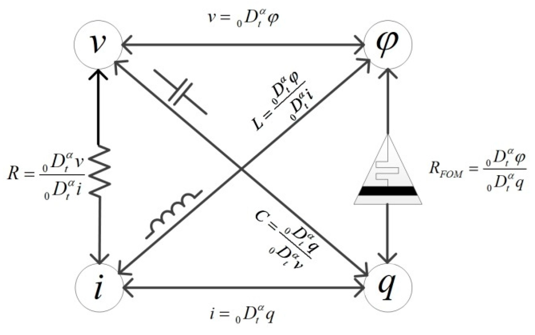
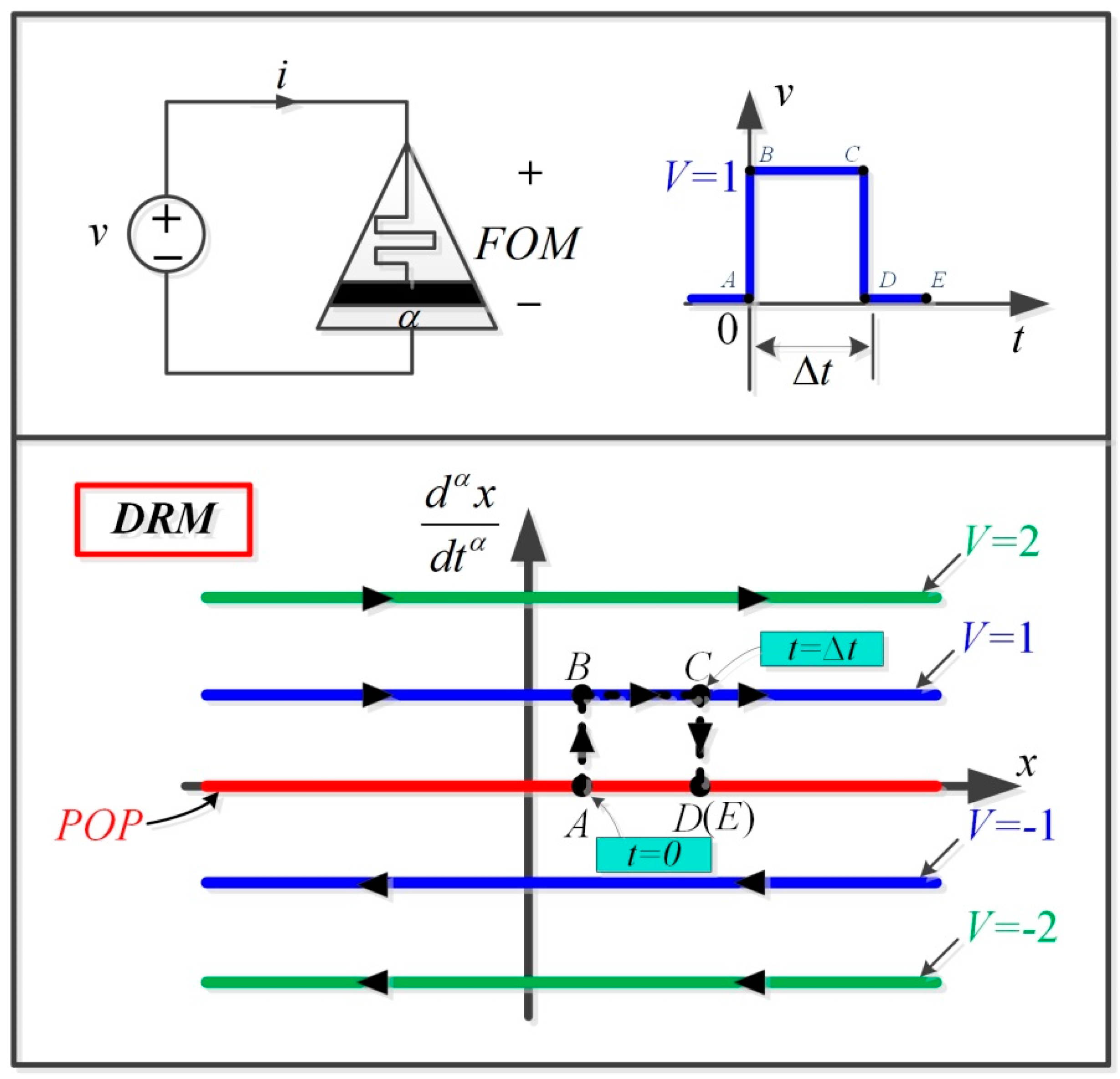
2.1. Fractional Order Memristor Model

Memristors can be divided into two types [17]: current control and voltage control. The mathematical expression of the voltage-controlled memristor is as follows:
i ( t ) = G ( x , v , t ) v ( t ) x ˙ = f ( x , v , t )
where v ( t ) , i ( t ) , and x are the voltage, the current, and the state variables of the memristor, respectively.
A fractional order voltage controlled memristor can be defined as follows [18]:
i ( t ) = G ( x , v , t ) v ( t ) 0 D t α x ( t ) = f ( x , v , t ) ( α > 0 )
where 0 D t α is fractional order arithmetic operator; α denotes fractional order; and 0 and t represent integral range. The fractional arithmetic operator can evolve into the following forms [34]:
0 D t α = { d α d t α α > 0 1 α = 0 0 t ( d τ ) α α < 0
In order to describe the memory effect of HP titanium dioxide memristors more effectively, a fractional order titanium dioxide memristor model is proposed in Reference [19]. The relationship between the internal state variable x ( t ) and current i ( t ) of the memristor is explained by fractional order calculus. The fractional derivative is defined in the form of Caputo derivative [35]:
D t α 0 C u ( t ) = 1 Γ ( m α ) 0 t u ( m ) ( τ ) ( t τ ) 1 + α m d τ
where Γ ( m ) is a Gamma function and m is the smallest integer not less than α .
A novel fractional derivative memristor model based on Caputo derivative is proposed as follows:
i ( t ) = G ( x ( t ) ) v ( t ) = ( a + b x ( t ) 2 ) v ( t ) D t α 0 C x ( t ) = v ( t ) ( α > 0 )
We take the driving voltage as v ( t ) = V sin ( ω t ) , i.e.,
D 0 C t α x ( t ) = V 0 sin ( ω t ) ( α > 0 )
Based on Equation (6), according to the properties of Caputo fractional derivative [35], i.e.,
D t 1 α 0 C ( D 0 C t α x ( t ) ) = x ˙ ( t ) , α ( 0 , 1 )
D t α 0 C ( D 0 t α x ( t ) ) = x ( t )
it can be deduced that
x ˙ ( t ) = V D t 1 α 0 C sin ( ω t )
D t α 0 C sin ( ω t ) V D t α C sin ( ω t ) = ω α sin ( ω t + α 2 π )
Combining Equations (9) and (10), Equation (11) can be obtained:
x ˙ ( t ) V ω 1 α sin ( ω t + 1 α 2 π )
Integrate both sides of Equation (11), i.e.,
x ( t ) x ( 0 ) + V ω α [ cos ( 1 α 2 π ) cos ( ω t + 1 α 2 π ) ]
By substituting Equation (12) into Equation (5), the following results can be obtained:
i ( t ) = { a + b [ x ( 0 ) + V ω α ( cos ( 1 α 2 π ) cos ( ω t + 1 α 2 π ) ) ] 2 } V sin ( ω t )
The symbols (plus or minus) of parameters a and b in Equation (13) can affect the passivity and activeness of the memristor and can consequently lead to corresponding changes in circuit characteristics. Compared with passive memristors, an active memristor is more suitable for use as second harmonic signal generation circuits [36]. Later, we will select the model with a < 0 and b < 0 for follow-up study.

2.2. Nonvolatility Analysis

According to the theory of nonvolatility of memristors, the phase diagram of the internal state variable derivative dx/dt and x of a memristor is called Power-Off Plot (referred to as POP) [37]. If there are two or more intersections between POP and x-axis, the memristor is nonvolatile.
The function equation satisfied by the power-off diagram of the fractional order memristor by Equation (5) is as follows:
d α x d t α = v | v = 0 = 0
As shown in the red line in Figure 1, the power-off plot overlaps with the x-axis—that is, at any moment of power failure, its fractional derivatives d α x / d t α are all 0—and the state variable x will remain at the time of power-off, showing that the memductance G ( x ( t ) ) of the memristor remains unchanged before and after power failure.
DRM (Dynamic Road Map) can reflect the change rule of state variable x of the fractional order memristor under different voltage, so as to understand the changes of memductance G ( x ( t ) ) and to prove the nonvolatility of fractional order memristor. Because of the linear relationship between d α x / d t α and v, the DRM graph is a straight line parallel to the horizontal axis. Figure 1 shows the collection of such dynamic routes parameterized by a voltage v. DRM has no backtracking characteristics; that is, any point on a dynamic route located above the x-axis must move to the right along the dynamic route because, for the fractional order rate of state variable x, d α x / d t α > 0 ( d α x / d t α is called fractional order rate in this paper) for any point on a dynamic route located in the upper half plane. x moves from left to right as time goes on; any point on the dynamic routes located below the x-axis must move to the left because d α x / d t α < 0 there.
If a voltage pulse signal with a width of Δ t and an amplitude of 1 V is applied to both ends of the memristor at a certain time, the state variable x of the memristor will jump from point A on the POP to point B on the parallel line of v = 1 V and then move to the right from point B to point C along the line in Δ t time. When the voltage pulse jumps to zero, the state variable will jump from point C to point D and remain unchanged at point D.
It follows that, regardless of the voltage value of the memristor at the time of interruption, the state variable x of the memristor can always remember the state before interruption, which proves that the memristor is nonvolatile.

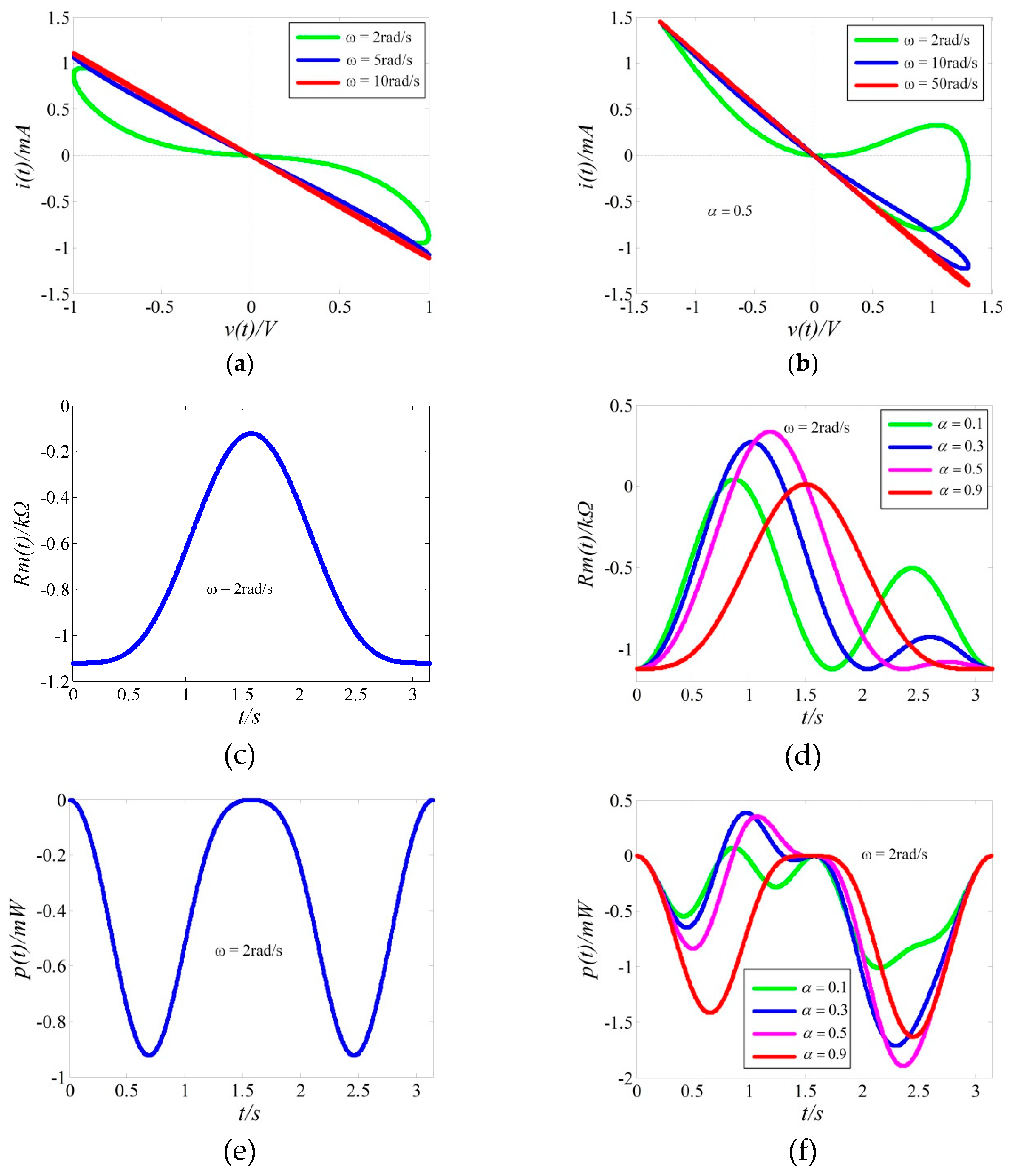
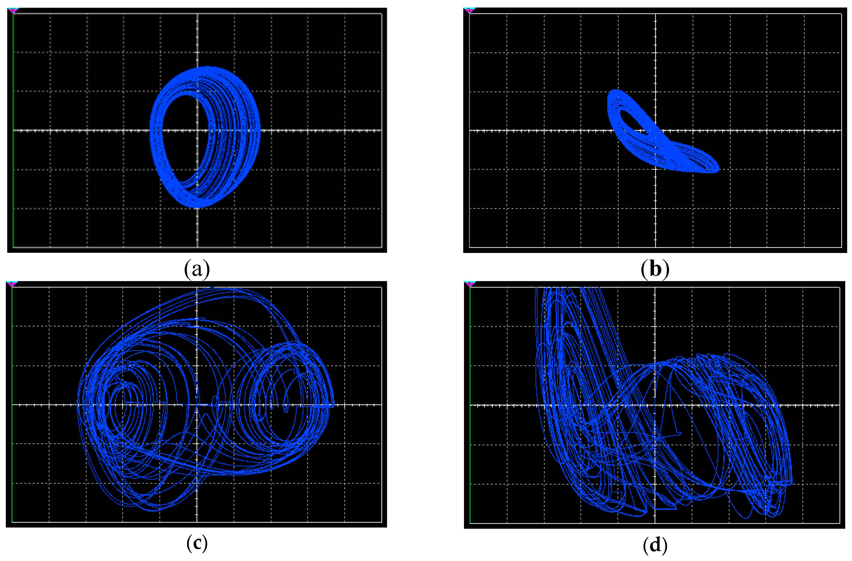
2.3. Numerical Simulations of the Memristor

Setting a = 1.12 , b = 1 , and v ( t ) = V sin ( ω t ) in Equation (13), the numerical simulation results of vi pinched hysteresis curve, memristance R m ( t ) , and instantaneous power p ( t ) are shown in Figure 2, in which Figure 2a,c,e shows the case of the integer order memristor and Figure 2b,d,f are the case of the fractional order memristor.
Comparing Figure 2a,b, it can be seen that the pinched hysteresis curves of the integer order memristors are located in the second and fourth quadrants and always present active characteristics, while the hysteresis curve of fractional order memristors is located in the first, second, and fourth quadrants under an excitation voltage, which shows that the local passive (or active) characteristics occur in a certain voltage range. With the increase of frequency ω , the memristors become an active linear resistor and the corresponding frequency of the fractional order memristor is obviously higher than that of the integer order memristor. Figure 2c shows that the integer order memristance is negative, which means that it is an active memristor, while the fractional order memristance of Figure 1d can change positively or negatively with time and is a local active or passive memristor. Figure 2e,f is an instantaneous power diagram, which shows that, when the memristance R m ( t ) 0 , there is always p ( t ) 0 , which corresponds to the activity of Figure 1c,d.

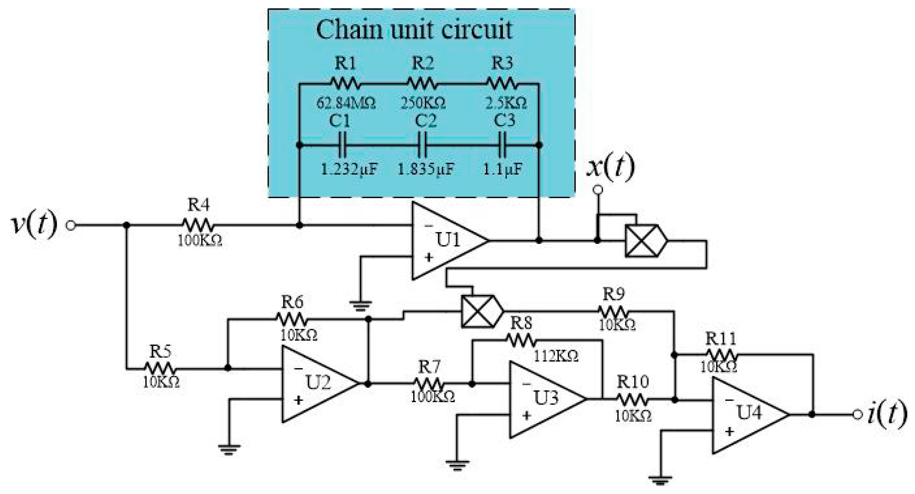
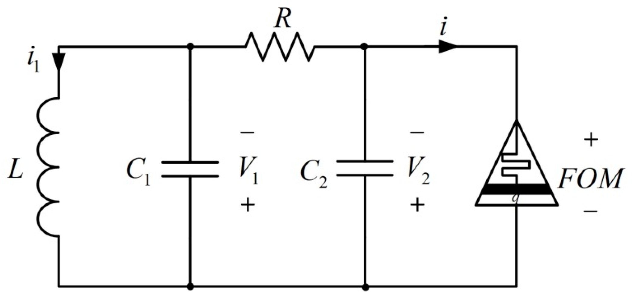
2.4. Equivalent Circuit of the Memristor

Setting the memristor model parameters proposed in Equation (5) as a = –1.12 and b = 1, we could obtain the following memductance equation:
i ( t ) = 1.12 v ( t ) + ( x ( t ) ) 2 v ( t ) x ( t ) = D 0 C t α v ( t ) ( α > 0 )
To obtain the fractional order memristor as described by Equation (15), an emulating circuit consisting of four operational amplifiers, two multipliers, and a chain cell circuit is designed as shown in Figure 3. The fractional calculus operation circuit is implemented by the method of time domain and complex frequency domain conversion. The fractional integral operator with order α is 1 / s α in complex frequency domain, and the chain unit circuit can realize the expansion of 1 / s α . When α = 0.9 , the resistances and the capacitances of the chain cell circuit in Figure 3 are taken as R 1 = 62.84 M Ω , R 2 = 250 K Ω , R 3 = 2.5 K Ω , C 1 = 1.232 μ F , C 2 = 1.835 μ F , and C 3 = 1.1 μ F [15,38]. The chain cell circuit is used to replace the capacitor in the common integration circuit to achieve fractional integration of order α = 0.9 , so we obtain x ( t ) = D t t 0 C v ( t ) in Figure 3. Three amplifiers U2, U3, and U4 and two multipliers constitute inverter circuits and adder circuits respectively. Equation (16) is the expression of the entire circuit, and the values of the rest of passive elements in Figure 3 can be obtained by comparing Equations (15) and (16).
i ( t ) = R 6 R 5 R 8 R 7 R 11 R 10 v ( t ) + R 11 R 9 ( x ( t ) ) 2 v ( t )
Figure 4a is the hysteresis curve of the memristor obtained by the Matlab numerical simulation where α = 0.9 . The hysteresis curve of the equivalent fractional order circuit in Figure 3 obtained by the circuit simulations using Multisim is shown in Figure 4b, in which the horizontal coordinate is the voltage signal v and the vertical coordinate is the current signal i. The simulation results of the circuit are consistent with those of the numerical simulation.

3. Fractional Order Memristor Based Chaotic Circuit

3.1. Mathematical Model

Fractional order models of basic circuit elements are more accurate than the corresponding integer order models and more suitable for describing the real world [39]. The relationship between fractional components is shown in Figure 5, in which resistors, capacitors, inductors, and memristors are all fractional order components.
If the voltage across the fractional order component is v ( t ) and the current flowing through it is i ( t ) , the voltage–ampere relationships of the fractional order capacitor and inductor can be deduced from Figure 4 as follows [40]:
C d α v ( t ) d t α = i ( t )
L d α i ( t ) d t α = v ( t )
In the second part, we show that the proposed fractional order memristor is locally active. Furthermore, it has been proven theoretically that the local activation of a device is the origin of complexity [41]. Its physical mechanism is the nonlinear amplification for weak signals in the local active region. Therefore, based on the fractional order memristor proposed in this paper, a chaotic circuit can be constructed and the oscillation can be maintained without the negative resistance to provide energy. The fractional order memristor-based chaotic circuit is shown in Figure 6, which is obtained from Chua’s circuit by replacing Chua’s diode with the fractional order memristor. All circuit elements in the circuit are fractional order devices.
According to Kirchhoff’s law, the state equations of the circuit in Figure 6 can be described by
{ d α i 1 d t α = v 1 L d α v 2 d t α = 1 C 2 [ v 1 v 2 R G ( x ) v 2 ] d α v 1 d t α = 1 C 1 [ v 2 v 1 R i 1 ] d α x d t α = v 2 ( α > 0 )
where D 0 c t α x ( t ) = v 2 ( α > 0 ) is memristor’s state equation obtained from Equation (5). Let x = i 1 , y = v 2 , z = v 1 , w = x , M = 1 / L , N = 1 / C 2 , 1 / C 1 = 1 , and R = 1 . Equation (19) can be rewritten as follows:
{ d α x d t α = M z d α y d t α = N [ ( z y ) G ( w ) y ] d α z d t α = y z x d α w d t α = y
If we set N = 10 and fractional order α = 0.9 , under the initial condition (0.18, 0.05, 0.02, and 0), the system is simulated by using the predictor–corrector algorithm [42] (step size 0.01, time range 1000 s), and the chaotic attractors of the system is obtained as shown in Figure 7, in which Figure 7a,b is the attractor trajectories in w-y and w-z phase spaces, respectively, when system parameter M = 16 , and Figure 7c,d is the attractor trajectories in w-y and w-z phase spaces, respectively, when system parameter M = 14 .

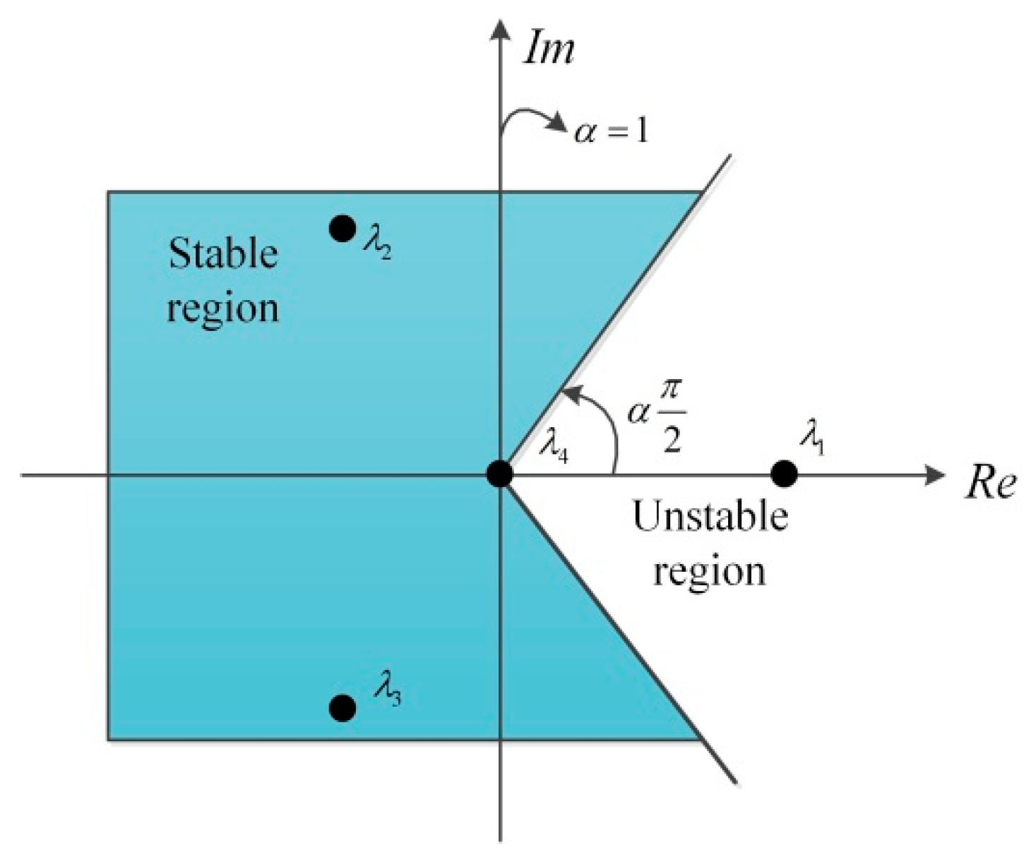
3.2. Equilibrium Points and Stability

Let d α x / d t α = d α y / d t α = d α z / d t α = d α w / d t α = 0 . We obtain the equilibria of Equation (20) as a set A = { ( x , y , z , w ) | x = y = z = 0 , w = c } where c is a real constant; that is, the circuit has an infinite set of points on w coordinates, which are all equilibrium points. The Jacobi matrix J is obtained by linearizing the Equation (20) at the equilibrium point set:
J = [ 0 0 M 0 0 N ( 1 + G ( w ) ) N 2 b N w y 1 1 1 0 0 1 0 0 ]
The corresponding characteristic equation is as follows:
λ 4 + [ 1 + N ( 1 + W ( c ) ) ] λ 3 + [ M + N W ( c ) ] λ 2 + M N [ 1 + W ( c ) ] λ = 0
where W ( c ) = a + b c 2 .
Let M = 13 , N = 10 , a = 1.12 , and b = 1 ; Equation (22) can be simplified to
λ [ λ 3 + ( 10 c 2 0.2 ) λ 2 + ( 10 c 2 + 1.8 ) λ + 130 c 2 15.6 ] = 0
For a fractional order linear system, if the eigenvalue λ i ( i = 1 , 2 , 3 , 4 ) at a certain equilibrium point satisfies | arg ( λ i ) | > α π / 2 , where α is a fractional order integral order, the system is asymptotically stable [43]. The necessary condition (stability criterion) for the system to be unstable at a certain equilibrium point is that the eigenvalue λ i satisfies the following:
| arg ( λ i ) | = | arg ( Re ( λ i ) + j Im ( λ i ) ) | α π / 2
It can be inferred that order α satisfies the following:
α > 2 π arctan | Im ( λ i ) | | Re ( λ i ) |
According to Equation (23), the eigenvalues of the system at the equilibrium point w = 0 can be calculated as λ 1 = 2.3207 , λ 2 , 3 = 1.0603 ± 2.3658 , and λ 4 = 0 . Taking α = 0.99 , we obtain α π / 2 = 1.551 and | arg ( λ i ) | = 0 , i.e., | arg ( λ i ) | < α π / 2 , which meets the stability criterion of Equation (24). The distribution of eigenvalues on the complex plane is shown in Figure 8, from which we observe that the points corresponding to eigenvalue λ 1 = 2.3207 are in the unstable region. Equation (24) is not a sufficient condition for stability, so the stability of the system at this equilibrium point needs further verification.
Taking α = 0.99 and ( x ( 0 ) , y ( 0 ) , z ( 0 ) , w ( 0 ) ) = ( 0 , 0 , 0.001 , 0 ) , the attractor trajectory of the system in the x-z phase plane is shown in Figure 9. The corresponding Lyapunov exponents [44] can be calculated: LE1 = 0.2607, LE2 = 0.009953, LE3 = −0.007345, and LE4 = −2.926. It follows that the system is in chaotic state, and it is unstable at the equilibrium point w = 0.
This fractional order memristor-based chaotic circuit has infinite equilibrium points (i.e., ( x e , y e , z e , w e ) = ( 0 , 0 , 0 , w ) , w = c , and c is an arbitrary real constant). The equilibrium points that are symmetric about w = 0 have the same characteristic roots and the same stability. Table 1 lists the circuit dynamics with equilibrium parameter w, eigenvalues, and fractional order α. In the fifth and sixth lines of Table 1, although the necessary conditions for the instability of fractional order linear systems are satisfied under this equilibrium point, the system is still in stable state according to the phase diagram of the attractor in Figure 10. Therefore, the stability of the equilibrium point of the fractional order system should be judged by calculating the stability criterion first and then by numerical simulation. The attractors that correspond to Table 1 are shown in Figure 10.

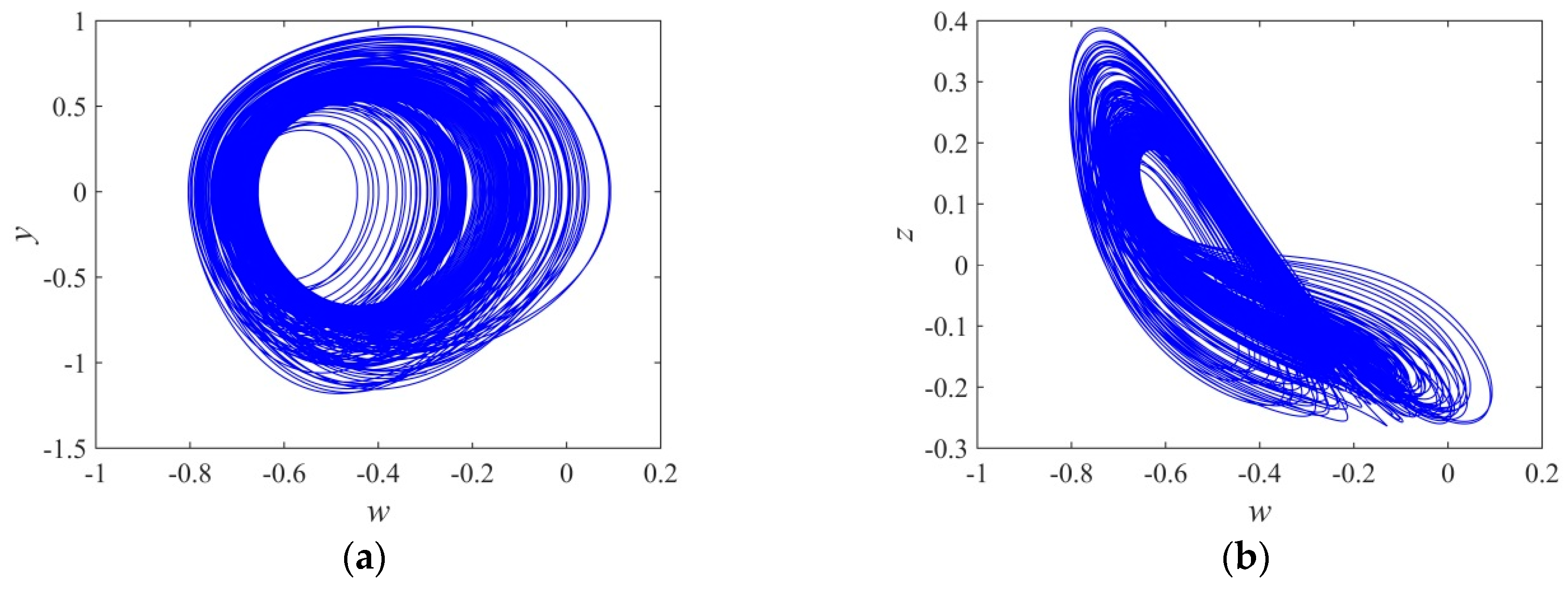
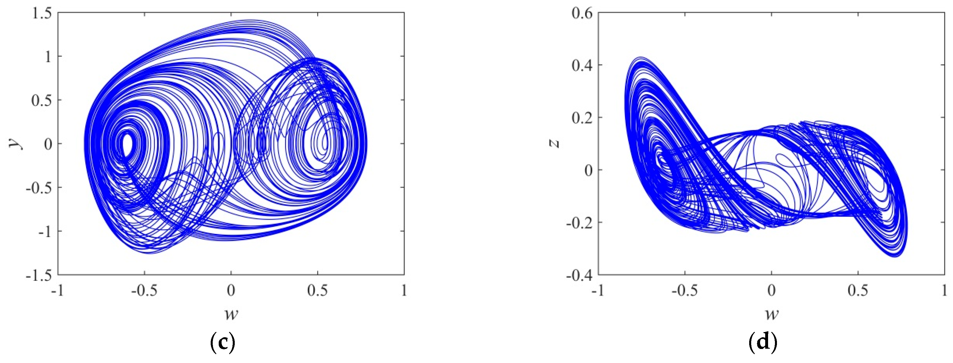
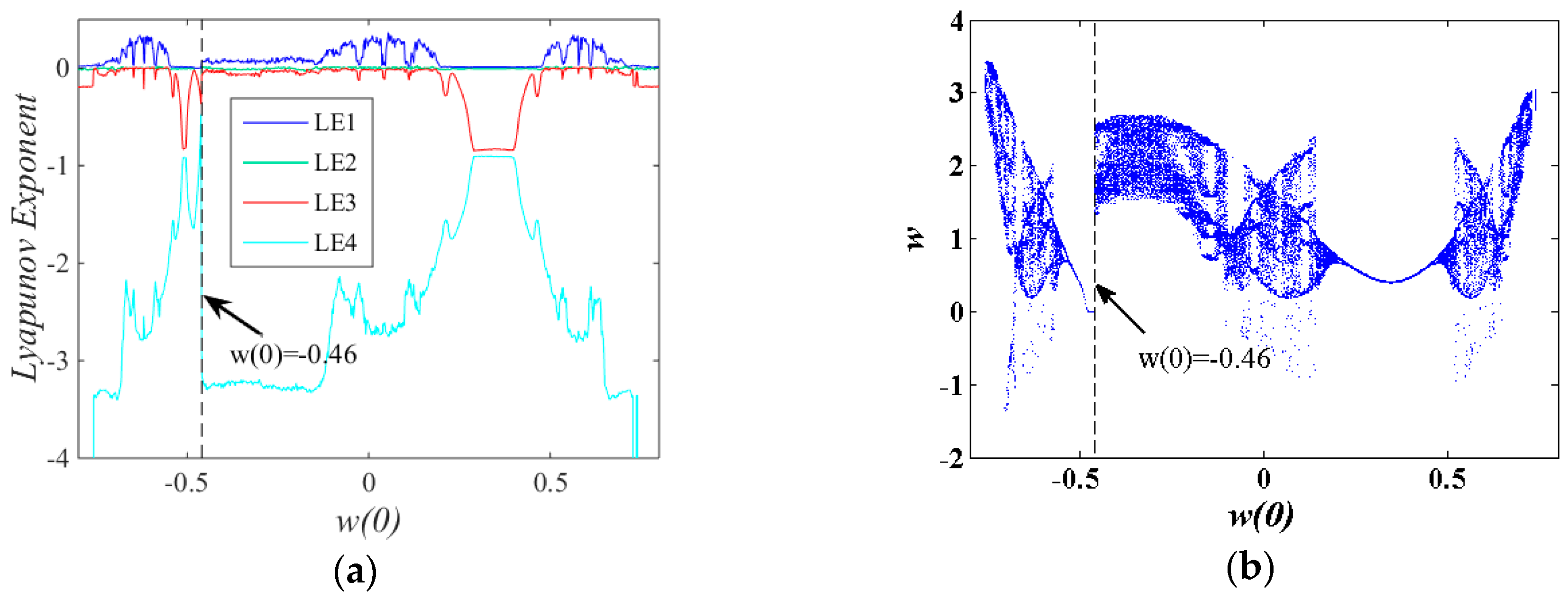
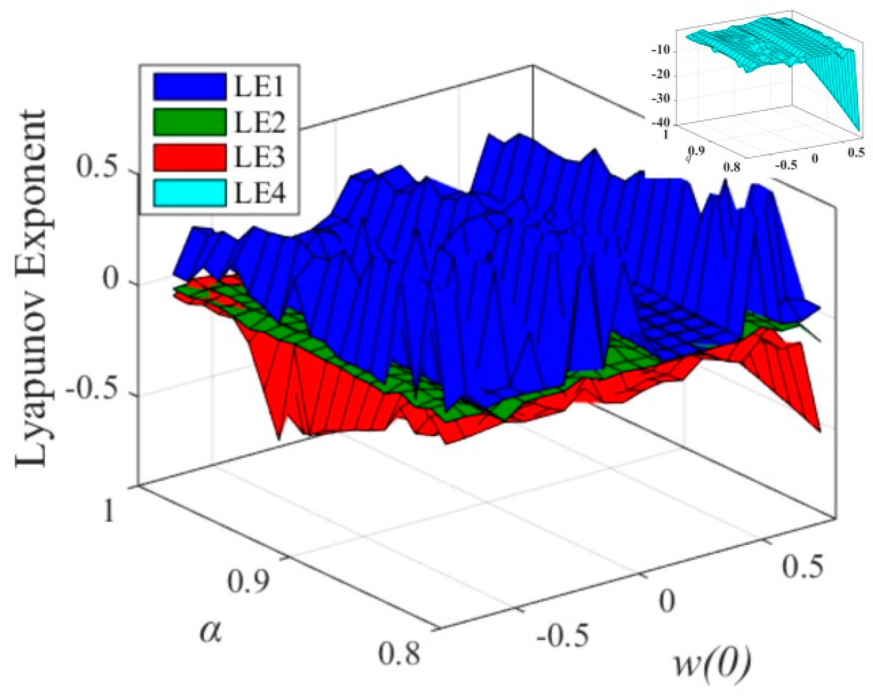
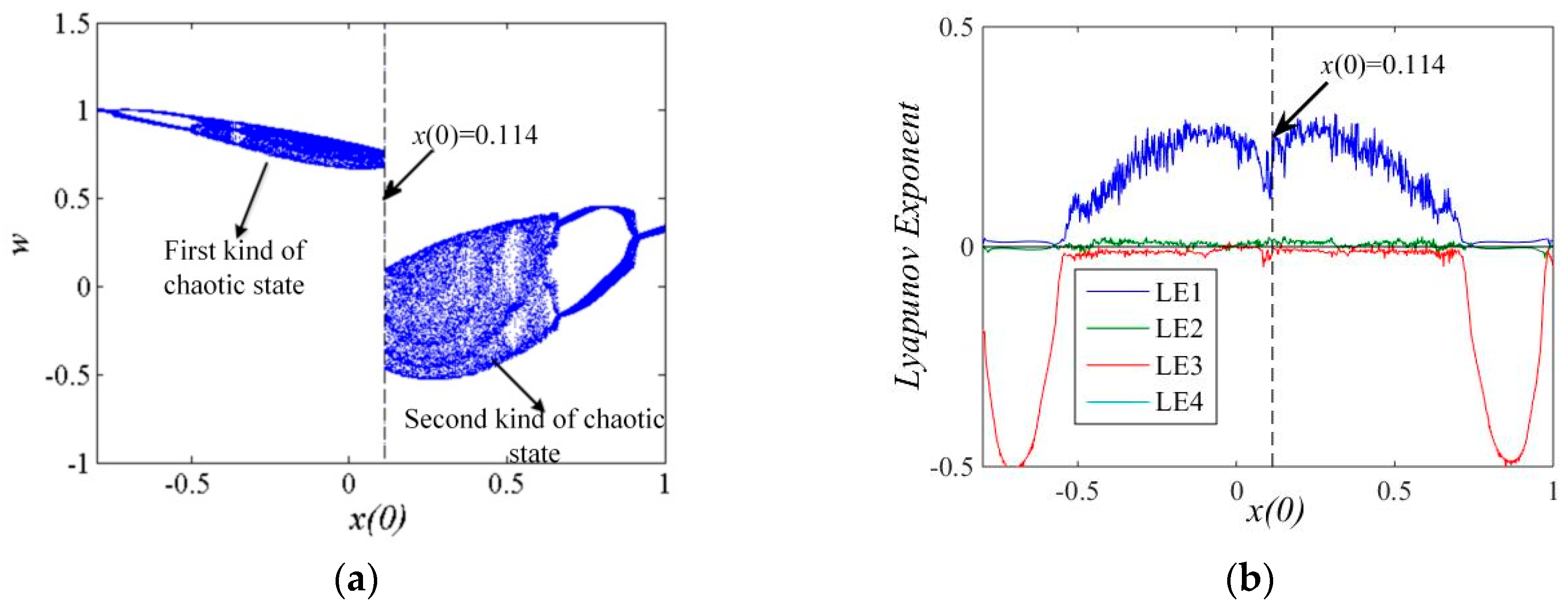
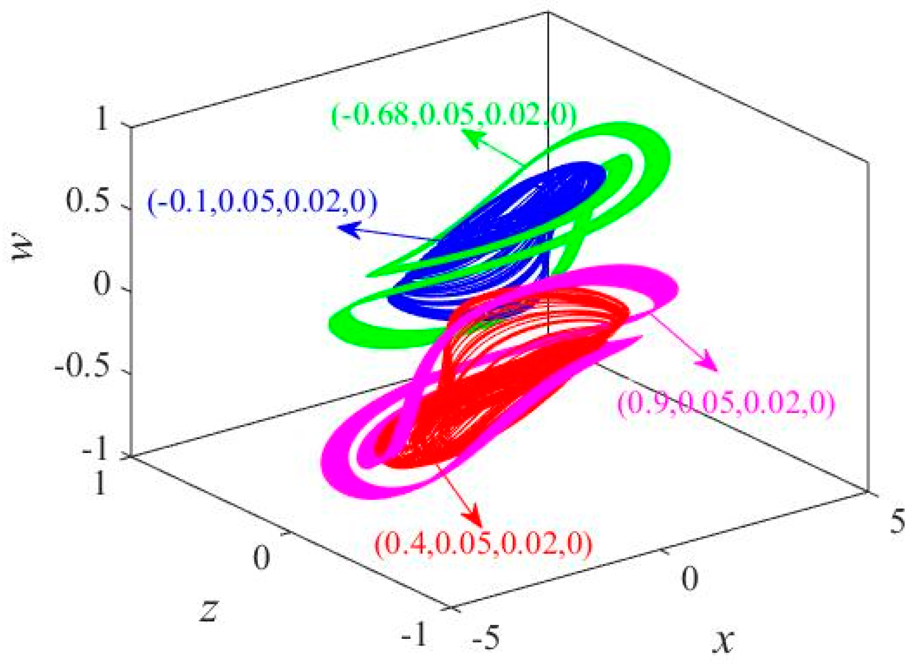
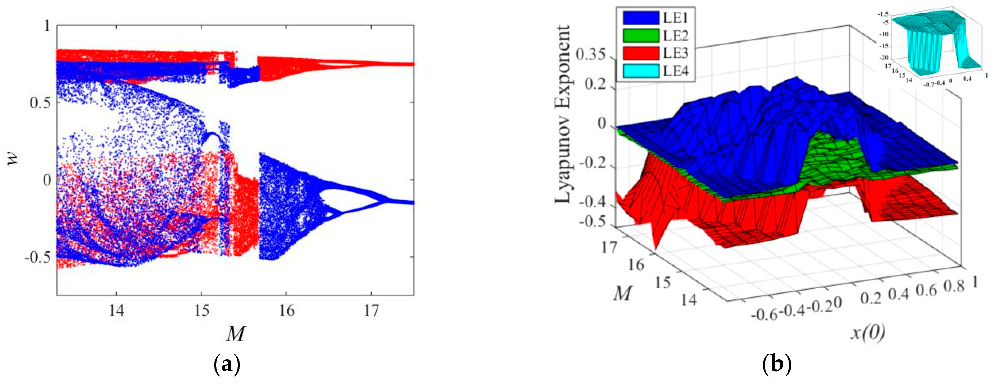
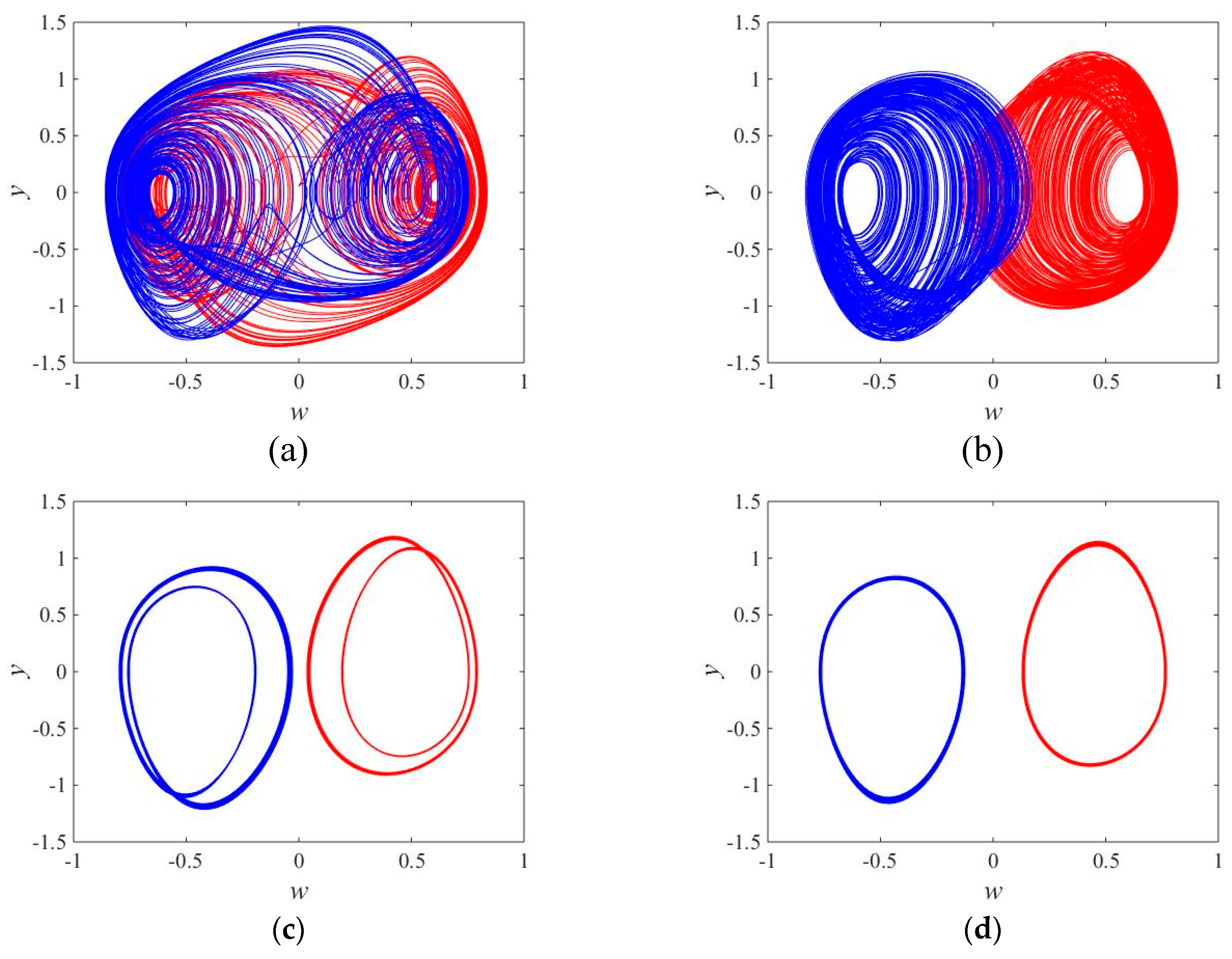
3.3. The Influence of Initial w(0) and Fractional Order α on Dynamics

Taking M = 15 , N = 10 , and α = 0.99 and fixing x ( 0 ) = 0 , y ( 0 ) = 0.05 , and z ( 0 ) = 0 , when initial value w ( 0 ) varies in the range of (−0.8 0.8), the Lyapunov exponent spectrum of the system is shown in Figure 11a and the corresponding bifurcation diagram with initial value w ( 0 ) is shown in Figure 11b. The ranges of the largest positive Lyapunov exponent in Figure 11a are 0.758 w ( 0 ) 0.546 , 0.46 w ( 0 ) 0.198 , and 0.478 w ( 0 ) 0.706 , which correspond to the three chaotic bands in Figure 11b.
Figure 12 shows the pinched hysteresis curves of the fractional order memristor on the v 2 i plane in the circuit shown in Figure 6. Figure 12a selects the initial value w ( 0 ) = 0.4 , which corresponds to a periodic attractor, and Figure 12b selects the initial value w ( 0 ) = 0.6 , which corresponds to a chaotic attractor, thereby exhibiting a chaotic pinched hysteresis curve.
The abovementioned system dynamics analysis is only based on fractional order α = 0.99 . However, parameter α will greatly affect the dynamics of the system. In order to visually reflect the cross influence of w ( 0 ) and α on the dynamic characteristics, Figure 13 shows the Lyapunov exponent surface of the system with initial value w ( 0 ) ( 0.8 , 0.8 ) and fractional order α ( 0.8 , 1 ) . The fourth Lyapunov surface of the system is reduced and placed on the upper right of the picture. Seen from the direction of w ( 0 ) axis, the part of the largest Lyapunov exponent LE1 surface larger than 0 is divided into three segments. The value of LE1 in the entire α-axis is greater than 0, which means that, when α ( 0.8 , 1 ) , the initial value w ( 0 ) is arbitrarily chosen in the three segments and the system is always chaotic.

3.4. Coexisting Bifurcation

Coexisting attractor refers to different types of attractors in the system when the initial value changes under the condition that the system parameters remain unchanged. The different bifurcations caused by different initial values is called coexisting bifurcation.
Fix the system parameters M = 16 and N = 10 and select the initial values y ( 0 ) = 0.05 , z ( 0 ) = 0 , w ( 0 ) = 0 , and x ( 0 ) ( 0.8 , 1 ) , then the bifurcation diagram and Lyapunov exponent spectrum of system variable w varying with initial value x ( 0 ) are shown in Figure 14a,b, respectively. For clarity, the fourth Lyapunov exponential curve in Figure 14b is not shown.
Compared with bifurcation graph and Lyapunov exponent spectrum, it can be found that, with the increase of initial value x ( 0 ) , the system enters the first kind of chaotic state from periodic state by a double-period bifurcation process. When x ( 0 ) value reaches 0.114, the system jumps from the first kind of chaotic state to the second kind of chaotic state and finally changes back to periodic state through an inverse double-period bifurcation process. These chaotic states and periodic orbits that appear as the initial value changes show that the system has many different coexisting attractors. Figure 15 shows four coexisting attractors in the x-z-w phase space; the corresponding initial values are annotated in the figure.
Figure 16a shows a coexisting bifurcation; that is, the system has two kinds of chaotic states with the change of initial value x ( 0 ) , where the red bifurcation diagram starts from the initial condition (0.01, 0.05, 0.02, 0), and the blue bifurcation diagram starts from the initial condition (0.18, 0.05, 0.02, 0). The evolution process of the two bifurcations shows that. with the increase of parameter M, the two chaotic attractors undergo inverse double-period bifurcation and eventually evolve into periodic states. Furthermore, the coexisting two bifurcations jump approximately at the interval of x ( 15.2 , 15.8 ) , which means that the spatial positions of the two chaotic attractors have changed during this bifurcation process.
The coexisting bifurcation phenomenon is closely related to initial value x ( 0 ) and system parameter M. Figure 16b shows a three-dimensional Lyapunov exponential spectral surface versus initial values x ( 0 ) and parameter M. Along the x-axis (resp., M-axis) direction, when a point on the LE1 surface is greater than zero, it shows that the system is chaotic under the current initial value x ( 0 ) (resp., M). The part where the LE1 surface is larger than zero is continuous and takes a larger proportion of the area, which means that the chaotic state of the system has a wider parameter range.
Figure 17 shows the coexisting attractors under the different initial values, where the red and the blue attractors correspond to the initial values (0.01, 0.05, 0.02, 0) and (0.18, 0.05, 0.02, 0), respectively. Figure 17a is a pair of coexisting double-scroll chaotic attractors in the w-y phase plane with parameter M = 16 , and Figure 17b is a pair of coexisting single-scroll chaotic attractors in the w-y phase plane with parameter M = 14 . A pair of coexisting period 2 attractors with parameter M = 16.8 is shown in Figure 17c, and a pair of coexisting periodic 1 attractors with M = 17.5 is shown in Figure 17d.

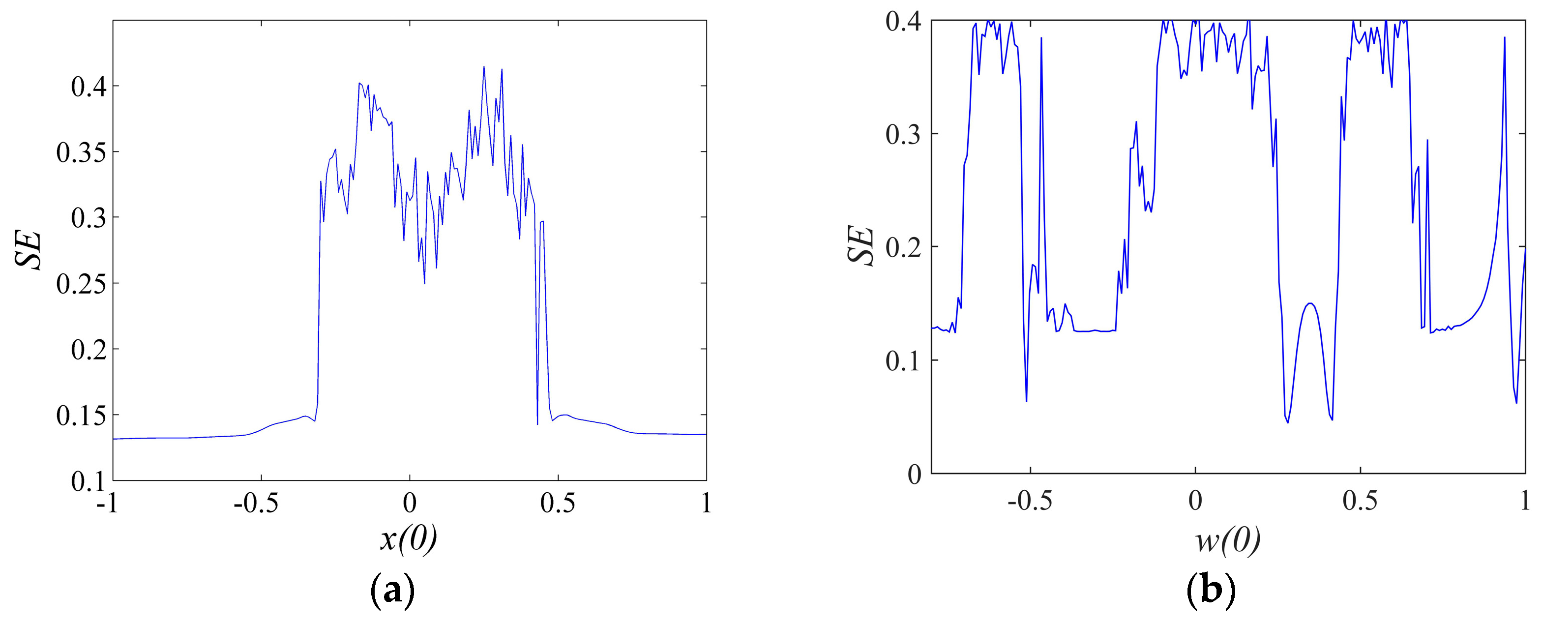
3.5. Spectral Entropy Analysis

SE (Spectral entropy) analysis can directly reflect the complexity of chaotic pseudorandom sequences [45]. In this section, spectral entropy analysis will be used to calculate the complexity of the fractional order system [46]. Calculation step length is 0.01 s and sequence length is 80,000 when α = 0.99 ; the complexity curve changing with the initial value of x ( 0 ) is shown in Figure 18a, and the complexity curve changing with the initial value of w ( 0 ) is shown in Figure 18b. By comparing the complexity curve of fractal order chaotic system with the Lyapunov exponent, it can be seen that the complexity curve is consistent with the Lyapunov exponent. When the system is in chaotic state, SE complexity is large, while when the system is in periodic state, SE complexity is small.

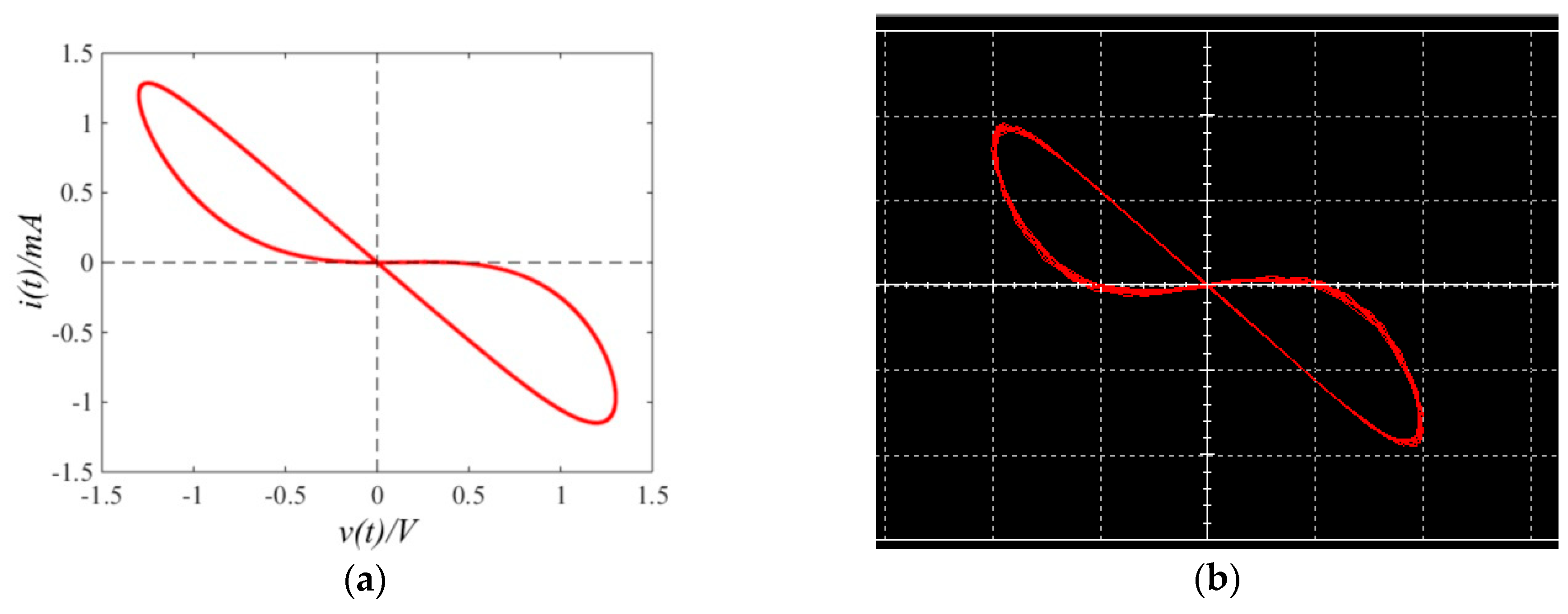
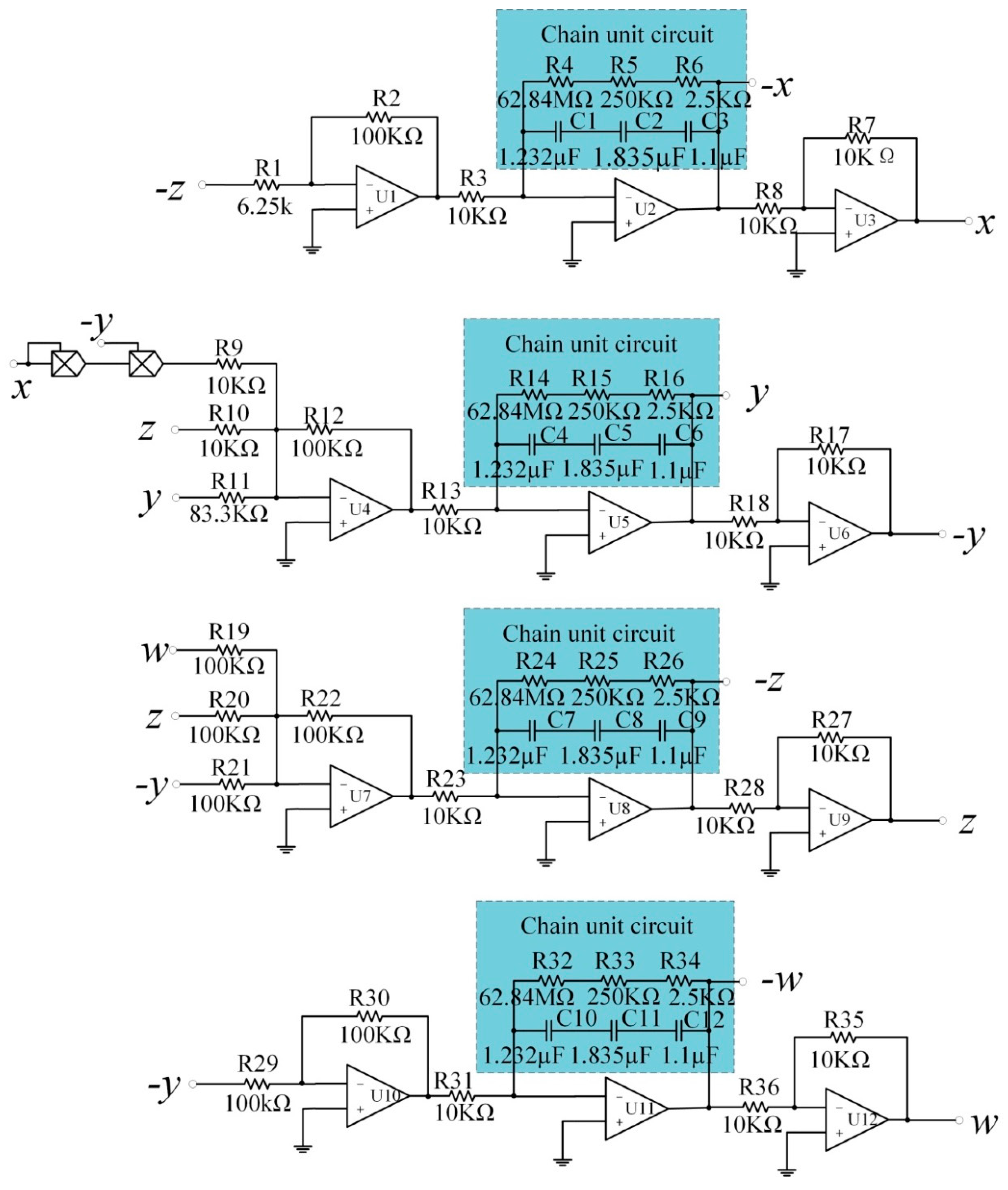
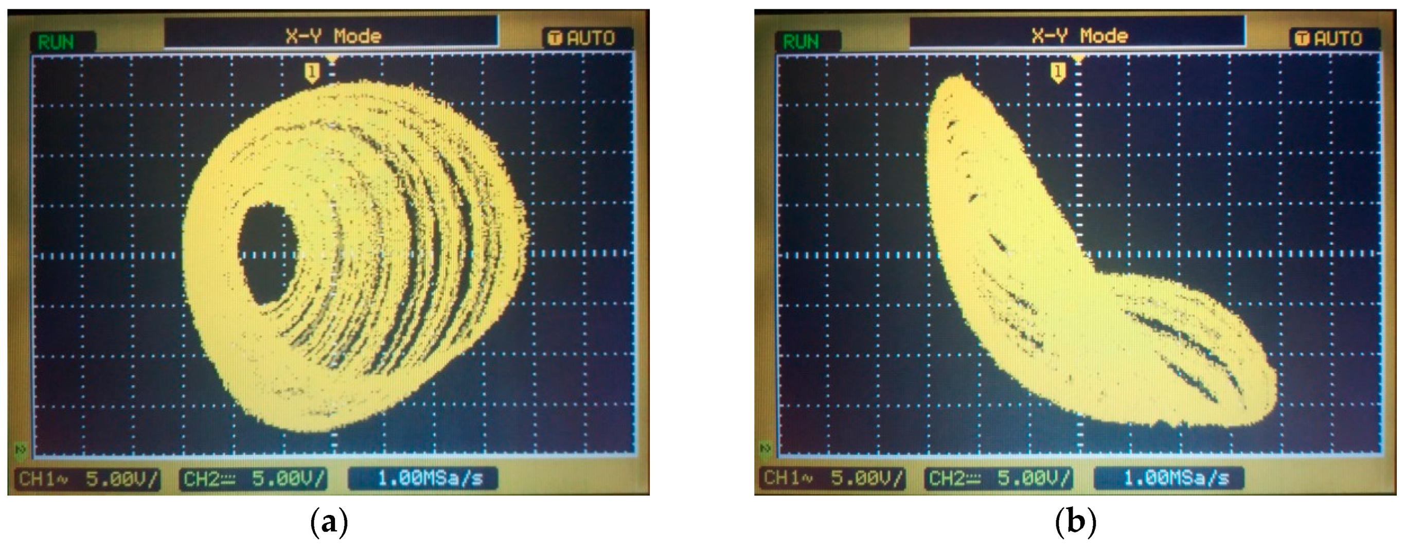
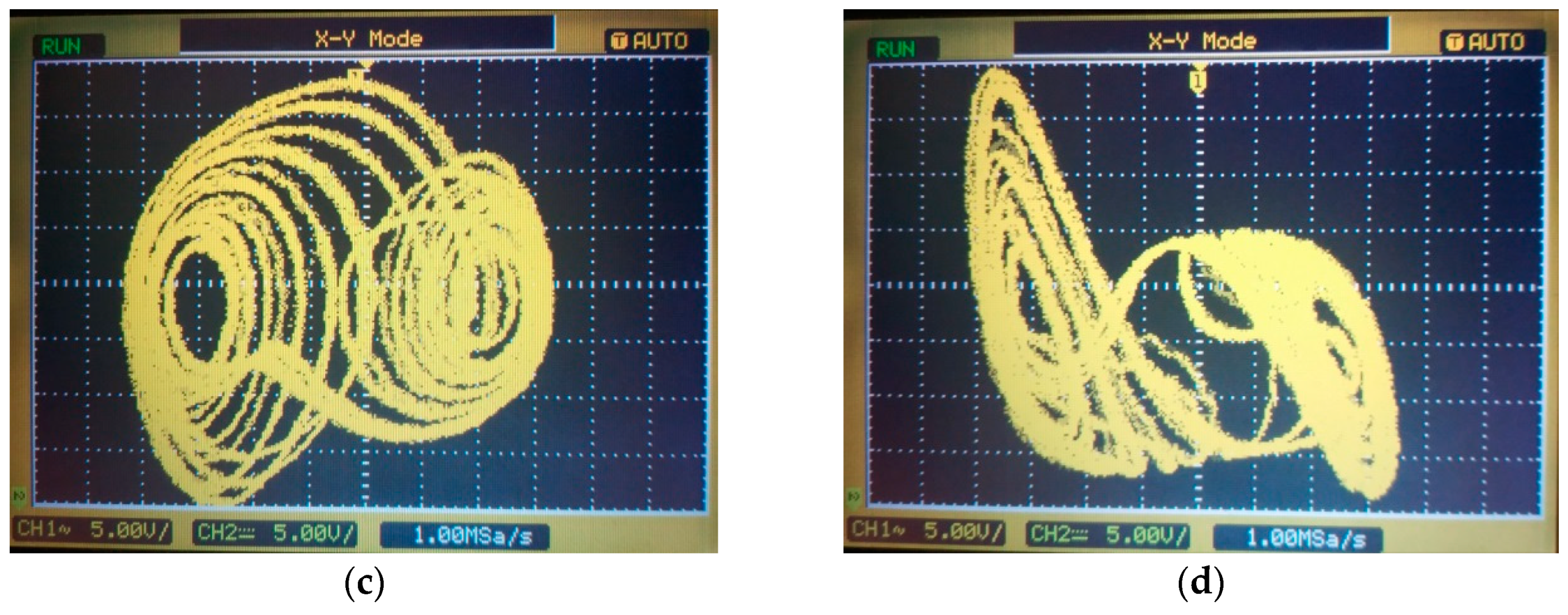
4. Experimental Verification

In order to verify the dynamic characteristics of the system, the circuit simulation experiment of the circuit is carried out by using Multisim circuit simulation software. Figure 19 is the schematic diagram designed by integrated operational amplifier circuits according to Equation (20), where α = 0.9 .
Figure 20 shows the experimental results of Figure 18 obtained by Multisim simulations. When R 1 = 6.25 K Ω and M = 16 , the phase diagrams of the single-scroll attractors in the w-y and w-z planes are shown in Figure 20a,b, respectively. Figure 20c,d show the double-scroll attractors in the w-y and w-z planes, respectively, where R 1 = 7.14 K Ω and M = 14 .
Due to the influence of the resistance and capacitance values in the chain cell circuit of the fractional integrators in Figure 18, it is difficult to realize the hardware analog circuit of the fractional order circuit. At present, most of the fractional order circuits are based on simulation experiments for verifying the circuit implementations. On the other hand, an analog circuit is not suitable for strict parameter matching and its performance is easily affected by environmental factors. Therefore, digital implementation of the fractional order circuit will be a better choice.
In our digital implementation, we choose a TMS320VC5509A 16-bit fixed-point type DSP (Digital signal processor) chip, the highest clock rate at 200 MHz, a 10-bit A/D maximum sampling rate at 21.5 KHz, ADC (Analog-to-digital converter) sample and hold acquisition time at 40 μ s , and ADC conversion time at 6500 ns . The A/D converter converts the chaotic sequence calculated by DSP into an analog signal, which can be output to an oscilloscope for observation. The power consumption of this digital implementation includes static power and active power. The static power consumption is 0.993 mW , the active power consumption is 93.894 mW , and the total power is 94.887 mW . Due to the limitation of DSP computational accuracy, some dynamic degradations will occur; the most well-problem is existence of many short-length chaotic orbits, which may weaken the complexity of chaotic sequence [47].
We adopt the Adomian decomposition algorithm [46] to design and implement the DSP digital simulation. The key to the decomposition of fractional order system by the Adomian method is to derive the coefficients of the series; the first six terms of the series are presented in the Appendix A. The flow chart of the implementation is shown in Figure 21, and the picture of the physical implementation is shown in Figure 22.
The digital simulation results of DSP with α = 0.9 are shown in Figure 23. Observe from Figure 20 and Figure 23 that the above two experimental results are in good agreement with the numerical simulation results, which shows that the dynamic theory analysis of the fractional order memristor based chaotic system in Section 3 is accurate.

5. Conclusions

We designed a fractional order memristor model by using theory of fractional differential equations. The nonvolatile, local-active, and local-passive characteristics have been verified via POP, DRM, and negative differential resistances. Based on the fractional order memristor, we constructed a fractional chaotic circuit, which possesses complex dynamical properties with respect to the fractional order α and can exhibit initial value dependent bifurcations and coexisting attractors. Simulations and DSP experiments verify the characteristics of the chaotic circuit.

Author Contributions

Investigation, W.Z.; methodology, J.W.; project administration, G.W.; validation, G.W. and H.H.-C.I.; writing—original draft, J.W.; writing—review and editing, J.W., G.W., and Y.S.

Funding

The work was supported by the National Natural Science Foundation of China under Grant (61771176).

Conflicts of Interest

The authors declare no conflict of interest.

Appendix A

The first six terms of the series are as follows:
C 1 1 = 16 C 3 0 , C 2 1 = 10 C 3 0 + 1.2 C 2 0 10 C 2 0 ( C 4 0 ) 2 , C 3 1 = C 2 0 C 3 0 C 1 0 , C 4 1 = C 2 0 ,
C 1 2 = 16 C 3 1 , C 2 2 = 10 C 3 1 + 1.2 C 2 1 20 C 2 0 C 4 0 C 4 1 10 C 2 1 ( C 4 0 ) 2 , C 3 2 = C 2 1 C 3 1 C 1 1 , C 4 2 = C 2 1 ,
C 1 3 = 16 C 3 2 , C 2 3 = 10 C 3 2 + 1.2 C 2 2 20 C 2 0 C 4 0 C 4 2 10 C 2 2 ( C 4 0 ) 2 ( 10 C 2 0 ( C 4 1 ) 2 + 20 C 2 1 C 4 0 C 4 1 ) Γ ( 2 q + 1 ) Γ 2 ( q + 1 ) , C 3 3 = C 2 2 C 3 2 C 1 2 , C 4 3 = C 2 2 ,
C 1 4 = 16 C 3 3 , C 2 4 = 10 C 3 3 + 1.2 C 2 3 20 C 2 0 C 4 0 C 4 3 10 C 2 3 ( C 4 0 ) 2 ( 20 C 2 0 C 4 1 C 4 2 + 20 C 2 1 C 4 0 C 4 2 + 20 C 2 2 C 4 0 C 4 1 ) Γ ( 3 q + 1 ) Γ ( q + 1 ) Γ ( 2 q + 1 ) 10 C 2 1 ( C 4 1 ) 2 Γ ( 3 q + 1 ) Γ 2 ( q + 1 ) , C 3 4 = C 2 3 C 3 3 C 1 3 , C 4 4 = C 2 3 ,
C 1 5 = a C 3 4 , C 2 5 = 10 C 3 4 + 1.2 C 2 4 20 C 2 0 C 4 0 C 4 4 10 C 2 4 ( C 4 0 ) 2 ( 20 C 2 0 C 4 1 C 4 3 + 20 C 2 1 C 4 0 C 4 3 + 20 C 2 3 C 4 0 C 4 1 ) Γ ( 4 q + 1 ) Γ ( q + 1 ) Γ ( 3 q + 1 ) ( 10 C 2 0 ( C 4 2 ) 2 + 20 C 2 2 C 4 0 C 4 2 ) Γ ( 4 q + 1 ) Γ 2 ( 2 q + 1 ) ( 20 C 2 1 C 4 1 C 4 2 + 10 C 2 2 ( C 4 1 ) 2 ) Γ ( 4 q + 1 ) Γ 2 ( q + 1 ) Γ ( 2 q + 1 ) , C 3 5 = C 2 4 C 3 4 C 1 4 , C 4 5 = C 2 4 ,
C 1 6 = a C 3 5 , C 2 6 = 10 C 3 5 + 1.2 C 2 5 20 C 2 0 C 4 0 C 4 5 10 C 2 5 ( C 4 0 ) 2 ( 20 C 2 0 C 4 1 C 4 4 + 20 C 2 1 C 4 0 C 4 4 + 20 C 2 4 C 4 0 C 4 1 ) Γ ( 5 q + 1 ) Γ ( q + 1 ) Γ ( 4 q + 1 ) ( 10 C 2 0 ( C 4 2 ) 2 + 20 C 2 2 C 4 0 C 4 2 ) Γ ( 4 q + 1 ) Γ 2 ( 2 q + 1 ) ( 20 C 2 0 C 4 2 C 4 3 + 20 C 2 2 C 4 0 C 4 3 + 20 C 2 3 C 4 0 C 4 2 ) Γ ( 5 q + 1 ) Γ ( 2 q + 1 ) Γ ( 3 q + 1 ) ( 20 C 2 1 C 4 1 C 4 3 + 10 C 2 3 ( C 4 1 ) 2 ) Γ ( 5 q + 1 ) Γ 2 ( q + 1 ) Γ ( 3 q + 1 ) ( 20 C 2 2 C 4 1 C 4 2 + 10 C 2 1 ( C 4 2 ) 2 ) Γ ( 5 q + 1 ) Γ 2 ( 2 q + 1 ) Γ ( q + 1 ) , C 3 6 = C 2 5 C 3 5 C 1 5 , C 4 6 = C 2 5 ,

References

  1. Chua, L.O. Memristor-The missing circuit element. IEEE Trans. Circuit Theory 1971, 18, 507–519. [Google Scholar] [CrossRef]
  2. Strukov, D.B.; Snider, G.S.; Stewart, D.R. The missing memristor found. Nature 2008, 453, 80–83. [Google Scholar] [CrossRef] [PubMed]
  3. Kumar, S.; Strachan, J.P.; Williams, R.S. Chaotics dynamics in namoscale NbO2 Mott memristors for analogue computing. Nature 2017, 548, 318–321. [Google Scholar] [CrossRef] [PubMed]
  4. Yuan, F.; Wang, G.Y.; Wang, X.Y. Dynamical characteristics of HP memristor based on equivalent circuit model in chaotic oscillator. Chin. Phys. B 2015, 24, 207–215. [Google Scholar] [CrossRef]
  5. Liu, G.Z.; Zheng, L.J.; Wang, G.Y. A carry lookahead adder based on hybrid CMOS-Memristor logic circuit. IEEE Access 2018, 7, 43691–43696. [Google Scholar] [CrossRef]
  6. Ma, D.; Wang, G.; Han, C.; Shen, Y.; Liang, Y. A memristive neural network model with associative memory for modeling affections. IEEE Access 2018, 6, 61614–61622. [Google Scholar] [CrossRef]
  7. Bertschinger, N.; Natschläger, T. Real-Time computation at the edge of chaos in recurrent neural networks. Neural Comput. 2004, 16, 1413–1436. [Google Scholar] [CrossRef] [PubMed]
  8. Buscarino, A.; Fortuna, L.; Frasca, M. A chaotic circuit based on Hewlett-Packard memristor. Chaos 2012, 22, 023136. [Google Scholar] [CrossRef]
  9. Itoh, M.; Chua, L.O. Memristor oscillators. Int. J. Bifurcat. Chaos 2008, 18, 3183–3206. [Google Scholar] [CrossRef]
  10. Wen, S.P.; Huang, T.; Zeng, Z. Adaptive synchronization of memristor-based Chua’s circuits. Phys. Lett. A 2012, 376, 2775–2780. [Google Scholar] [CrossRef]
  11. Li, Z.J.; Zeng, Y.C. A memristor oscillator based on a twin-T network. Chin. Phys. B 2013, 22, 040502. [Google Scholar] [CrossRef]
  12. Bao, B.C.; Xu, J.P.; Liu, Z. Initial state dependent dynamical behaviors in a memristor based chaotic circuit. Chin. Phys. Lett. 2010, 27, 51–53. [Google Scholar]
  13. Jin, P.P.; Wang, G.Y.; Iu, H.H.C. A locally-active memristor and its application in chaotic circuit. IEEE Trans. Circ. Syst. II Express Briefs 2017, 65, 246–250. [Google Scholar] [CrossRef]
  14. Chang, H.; Wang, Z.; Li, Y.X. Dynamic analysis of a bistable Bi-Local active memristor and its associated oscillator system. Int. J. Bifurcat. Chaos 2018, 28, 1850105. [Google Scholar] [CrossRef]
  15. Liu, C.X. Fractional-order Chaotic Circuit Theory and Applications; Xian Jiaotong University Press: Xi’an, China, 2011; pp. 61–65. [Google Scholar]
  16. Yu, Y.J.; Wang, Z.H. A fractional-order memristor model and the fingerprint of the simple series circuit including a fractional-order memrisotr. Acta Phys. Sin. 2015, 64, 238401. [Google Scholar]
  17. Ventra, M.D.; Pershin, Y.V.; Chua, L.O. Circuit elements with memory: Memristors, memcapacitors, and meminductors. Proc. IEEE 2009, 97, 1717–1724. [Google Scholar] [CrossRef]
  18. Petráš, I.; Chen, Y.Q. Fractional-Order Circuit Elements with Memory. In Proceedings of the 13th International Carpathian Control Conference, High Tatras, Slovakia, 28–31 May 2012; pp. 552–558. [Google Scholar]
  19. Fouda, M.E.; Ranwan, A.G. On the fractional-order memristor model. J. Fract. Calc. Appl. 2013, 4, 1–7. [Google Scholar]
  20. Fouda, M.E.; Ranwan, A.G. Fractional-order memristor response under DC and periodic signals. Circ. Syst. Singal Process. 2014, 34, 961–970. [Google Scholar] [CrossRef]
  21. Rashad, S.H.; Hamed, E.M.; Fouda, M.E. On the Analysis of Current-Controlled Fractional-Order Memristor Emulator. In Proceedings of the 6th International Conference on Modern Circuits and Systems Technologies, Thessaloniki, Greece, 4–6 May 2017. [Google Scholar]
  22. Hamed, E.M.; Fouda, M.E.; Radwan, A.G. Conditions and emulation of double pinch-off points in fractional-order memristor. In Proceedings of the IEEE International Symposium on Circuits and Systems, Florence, Italy, 27–30 May 2018. [Google Scholar]
  23. Elsafty, A.H.; Hamed, E.M.; Fouda, M.E.; Said, L.A.; Madian, A.H. Study of fractional flux-controlled memristor emulator connections. In Proceedings of the 7th International Conference on Modern Circuits and Systems Technologies, Thessaloniki, Greece, 7–9 May 2018. [Google Scholar]
  24. Yuan, F.; Li, Y.X.; Wang, G.Y.; Dou, G. Complex dynamics in a memcapacitor-based circuit. Entropy 2019, 21, 188. [Google Scholar] [CrossRef]
  25. Song, Y.X.; Yuan, F.; Li, Y.X. Coexisting attractors and multistability in a simple memristive wien-bridge chaotic circuit. Entropy 2019, 21, 678. [Google Scholar] [CrossRef]
  26. Pham, V.T.; Kingni, S.T.; Volos, C.; Jafari, S.; Kapitaniak, T. A simple three-dimensional fractional-order chaotic system without equilibrium: Dynamics, circuitry implementation, chaos control and synchronization. AEU-Int. J. Electron. Commun. 2017, 78, 220–227. [Google Scholar] [CrossRef]
  27. Petráš, I. Fractional-order memristor-based chua’s circuit. IEEE Trans. Circuits Syst. II Express Briefs 2011, 57, 975–979. [Google Scholar] [CrossRef]
  28. Cafagna, D.; Grassi, G. On the simplest fractional-order memristor-based chaotic system. Nonlinear Dyn. 2012, 70, 1185–1197. [Google Scholar] [CrossRef]
  29. Yu, Y.J.; Wang, Z.H. Initial state dependent nonsmooth bifurcations in a fractional-order memristive circuit. Int. J. Bifurcat. Chaos 2018, 28, 1850091. [Google Scholar] [CrossRef]
  30. Hajipour, A.; Tavakoli, H. Analysis and circuit simulation of a novel nonlinear fractional incommensurate order financial system. Optik 2016, 127, 10643–10652. [Google Scholar] [CrossRef]
  31. David, S.A.; Fischer, C.; Machado, J.T. Fractional electronic circuit simulation of a nonlinear macroeconomic model. AEU-Int. J. Electron. Commun. 2019, 84, 210–220. [Google Scholar] [CrossRef]
  32. Yang, N.N.; Xu, C.; Wu, C.J.; Jia, R. Modeling and analysis of a fractioanl-order generalized memristor-based chaotic system and circuit implementation. Int. J. Bifurcat. Chaos 2017, 27, 1750199. [Google Scholar] [CrossRef]
  33. Corinto, F.; Ascoli, A. A boundary condition-based approach to the modeling of memristor nanostructures. IEEE Trans. Circuits Syst. I Regul. Rap. 2012, 59, 2713–2726. [Google Scholar] [CrossRef]
  34. Oldham, K.B.; Spanier, J. The Fractional Calculus; Academic Press: New York, NY, USA, 1974; pp. 396–400. [Google Scholar]
  35. Caputo, M. Linear models of dissipation whose Q is almost frequency independent. Ann. Geophys. 1966, 19, 529–539. [Google Scholar] [CrossRef]
  36. Hu, F.W.; Bao, B.C.; Wu, H.G. Equivalent circuit analysis model of charge-controlled memristor and its circuit characteristics. Acta Phys. Sin. 2013, 62, 218401. [Google Scholar]
  37. Chua, L.O. Five non-volatile memristor enigmas solved. Appl. Phys. A 2018, 124, 563. [Google Scholar] [CrossRef]
  38. Zouad, F.; Kemih, K.; Hamiche, H. A new secure communication scheme using fractional order delayed chaotic system: Design and electronics circuit simulation. Analog Integr. Circuits Signal Process. 2019, 99, 619–632. [Google Scholar] [CrossRef]
  39. Hilfer, R. Applications of Fractional Calculus in Physics; World Scientific Publishing Co.: Munich, Germany, 2000; pp. 331–463. [Google Scholar]
  40. Westerlund, S. Dead matter has memory! Phys. Scr. 1991, 43, 174–179. [Google Scholar] [CrossRef]
  41. Chua, L.O. Loacl Activity is the origin of complexity. Int. J. Bifurcat. Chaos 2005, 15, 3435–3456. [Google Scholar] [CrossRef]
  42. Diethelm, K.; Ford, N.J.; Freed, A.D. A predictor-corrector approach for the numerical solution of fractional differential equations. Nonlinear Dyn. 2002, 29, 3–22. [Google Scholar] [CrossRef]
  43. Chen, L.P.; He, Y.G.; Lv, X.; Wu, R.C. Dynamic behaviours and control of fractional-order memristor-based system. Pramana 2015, 85, 91–104. [Google Scholar] [CrossRef]
  44. Marius-F, D.; Nikolay, K. Matlab code for lyapunov exponents of fractional-order systems. Inter. J. Bifurcat. Chaos 2018, 28, 1850067. [Google Scholar]
  45. Sun, K.H.; He, S.B.; He, Y.; Yin, L.Z. Complexity analysis of chaotic pseudo-random sequences based on spectral entropy algorithm. Acta Phys. Sin. 2013, 62, 010501. [Google Scholar]
  46. He, S.B.; Sun, K.H.; Wang, H.H. Solution of the fractional-order chaotic system based on adomian decomposition algorithm and its complexity analysis. Acta Phys. Sin. 2014, 63, 2965–2973. [Google Scholar]
  47. Gonzalo, A.; Li, S.J. Some basic cryptographic requirements for chaos-based cryptosystems. Int. J. Bifurcat. Chaos 2006, 16, 2129–2151. [Google Scholar]
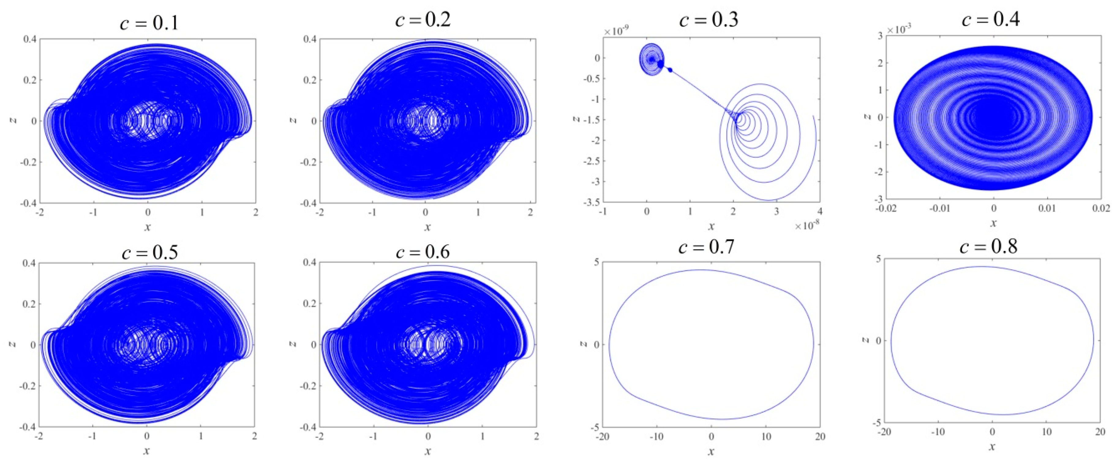
Figure 1. Dynamic Road Map (DRM) of the fractional order memristor.
Entropy 21 00955 g001
Figure 2. Numerical simulations of the integer order memristor: (a) pinched hysteresis loop, (c) memristance, and (e) instantaneous power and numerical simulations of the fractional order memristor: (b) the influence of fractional order on pinched hysteresis loop, (d) the influence of fractional order on memristance, and (f) the influence of fractional order on instantaneous power.
Entropy 21 00955 g002
Figure 3. Equivalent circuit of the fractional order memristor.
Entropy 21 00955 g003
Figure 4. The v − i hysteresis curves of the fractional order memristor with order α = 0.9 : (a) The Matlab numerical simulation and (b) Multisim circuit simulation.
Entropy 21 00955 g004
Figure 5. Fractional order components diagram.
Entropy 21 00955 g005
Figure 6. Fractional order memristor-based chaotic circuit.
Entropy 21 00955 g006
Figure 7. Chaotic attractors of the fractional system when α = 0.9 : (a) chaotic attractor in the w-y phase plane with M = 16 ; (b) chaotic attractor in the w-z phase plane with M = 16 ; (c) chaotic attractor in the w-y phase plane with M = 14 ; and (d) chaotic attractor in the w-z phase plane with M = 14 .
Entropy 21 00955 g007aEntropy 21 00955 g007b
Figure 8. Distribution of characteristic roots at the equilibrium point w = 0.
Entropy 21 00955 g008
Figure 9. Attractor in the x-z phase plane with α = 0.99 and ( x ( 0 ) , y ( 0 ) , z ( 0 ) , w ( 0 ) ) = ( 0 , 0 , 0.001 , 0 ) .
Entropy 21 00955 g009
Figure 10. Attractor trajectories of the system corresponding to different equilibrium points.
Entropy 21 00955 g010
Figure 11. Dynamic with w0, where α = 0.99 : (a) Lyapunov exponent spectrum; (b) bifurcation diagram.
Entropy 21 00955 g011
Figure 12. Pinched hysteresis curves of the fractional order memristor with initial value w ( 0 ) : (a) w ( 0 ) = 0.4 ; (b) w ( 0 ) = 0.6 .
Entropy 21 00955 g012
Figure 13. Lyapunov exponent spectrum with w ( 0 ) and α .
Entropy 21 00955 g013
Figure 14. Bifurcation diagram and Lyapunov exponent spectrum of w with initial value x ( 0 ) : (a) bifurcation diagram; (b) Lyapunov exponent spectrum.
Entropy 21 00955 g014
Figure 15. Coexisting attractors in x-z-w phase space.
Entropy 21 00955 g015
Figure 16. Coexisting bifurcation versus parameter M and initial values: (a) Coexisting bifurcations for initial conditions (0.01, 0.05, 0.02, 0) (red bifurcation diagram) and (0.18, 0.05, 0.02, 0) (blue bifurcation diagram); (b) three-dimensional Lyapunov exponent spectrum versus initial value x(0) and parameter M.
Entropy 21 00955 g016
Figure 17. Coexisting attractors where the red and the blue attractors correspond to the initial values (0.01, 0.05, 0.02, 0) and (0.18, 0.05, 0.02, 0), respectively: (a) M = 14 ; (b) M = 16 ; (c) M = 16.8 ; and (d) M = 17.5 .
Entropy 21 00955 g017
Figure 18. α = 0.99 , SE complexity curve with respect to initial values: (a) x ( 0 ) ( 1 , 1 ) ; (b) w ( 0 ) ( 0.8 , 1 ) .
Entropy 21 00955 g018
Figure 19. Schematic diagram of the fractional order memristor-based chaotic circuit.
Entropy 21 00955 g019
Figure 20. Chaotic attractors obtained by Multisim simulation experiments: (a) chaotic attractor in the w-y phase plane with M = 16 ; (b) chaotic attractor in the w-z phase plane with M = 16 ; (c) chaotic attractor in the w-y phase plane with M = 14 ; and (d) chaotic attractor in the w-z phase plane with M = 14 .
Entropy 21 00955 g020
Figure 21. The flow chart of the DSP digital implementation.
Entropy 21 00955 g021
Figure 22. The picture of the physical implementation.
Entropy 21 00955 g022
Figure 23. DSP experiment results of the fractional order circuit: (a) chaotic attractor in the w-y phase plane with M = 16 ; (b) chaotic attractor in the w-z phase plane with M = 16 ; (c) chaotic attractor in the w-y phase plane with M = 14 ; and (d) chaotic attractor in the w-z phase plane with M = 14 .
Entropy 21 00955 g023aEntropy 21 00955 g023b
Table 1. Dynamics with equilibrium parameter w, eigenvalues, and fractional order α ( α π / 2 = 1.551 )
w = c λ 1 λ 2 , 3 | a r g ( λ ) | α Dynamics
02.3207−1.0603 ± 2.3658i00.7318chaos
0.12.1972−1.0480 ± 2.3250i00.7304chaos
0.21.7968−0.9984 ± 2.1888i00.7275chaos
0.30.9268−0.8134 ± 1.8831i0stable point
0.4−1.47840.0393 ± 1.8748i1.5498stable point
0.5−2.86130.2807 ± 2.4140i1.45500.9263chaos
0.6−4.00000.3000 ± 2.7760i1.46320.9314chaos
0.7−5.19330.2466 ± 3.0333i1.48970.9484limit cycle
0.8−6.52960.1648 ± 3.2133i1.51950.9673limit cycle

