1. Introduction
Signal processing techniques are routinely applied in the great majority of security-oriented applications. In particular, the detection problem plays a fundamental role in many security-related scenarios, including secure detection and classification, target detection in radar-systems, intrusion detection, biometric-based verification, one-bit watermarking, steganalysis, spam-filtering, and multimedia forensics (see [
1]). A unifying characteristic of all these fields is the presence of an adversary explicitly aiming at hindering the detection task, with the consequent necessity of adopting proper models that take into account the interplay between the system designer and the adversary. Specifically, the adopted models should be able to deal, on the one hand, with the uncertainty that the designer has about the attack the system is subject to, and, on the other hand, with the uncertainty of the adversary about the target system (i.e., the system it aims at defeating). Game theory has recently been proposed as a way to study the strategic interaction between the choices made by the system designer and the adversary. Among the fields wherein such an approach has been used, we mention steganalysis [
2,
3], watermarking [
4], intrusion detection [
5] and adversarial machine learning [
6,
7]. With regard to binary detection, game theory and information theory have been combined to address the problem of adversarial detection, especially in the field of digital watermarking (see, for instance, [
4,
8,
9,
10]). In all these works, the problem of designing watermarking codes that are robust to intentional attacks is studied as a game between the information hider and the attacker.
An attempt to develop a general theory for the binary hypothesis testing problem in the presence of an adversary is made in [
11]. Specifically, in [
11], the general problem of binary decision under adversarial conditions is addressed and formulated as a game between two players, the
defender and the
attacker, which have conflicting goals. Given two discrete memoryless sources,
and
, the goal of the defender is to decide whether a given test sequence has been generated by
(null hypothesis,
) or
(alternative hypothesis,
). By adopting the Neyman–Pearson approach, the set of strategies the defender can choose from is the set of decision regions for
ensuring that the false positive error probability is lower than a given threshold. On the other hand, the ultimate goal of the attacker in [
11] is to cause a false negative decision, so the attacker acts under
only. In other words, the attacker modifies a sequence generated by
, in attempt to move it into the acceptance region of
. The attacker is subjected to a distortion constraint, which limits his freedom in doing so. Such a struggle between the defender and the attacker is modeled in [
11] as a competitive zero-sum game; the asymptotic equilibrium, i.e., the equilibrium when the length of the observed sequence tends to infinity, is derived under the assumption that the defender bases his decision on the analysis of first-order statistics only. In this respect, the analysis conducted in [
11] extends the one of [
12] to the adversarial scenario. Some variants of this attack-detection game have also been studied; for instance, in [
13], the setting is extended to the case where the sources are known to neither the defender nor the attacker, while the training data from both sources are available to both parties. Within this framework, the case where part of the training data available to the defender is corrupted by the attacker has also been studied (see [
14]).
The assumption that the attacker is active only under stems from the observation that in many cases corresponds to a kind of normal or safe situation and its rejection corresponds to revealing the presence of a threat or that something anomalous is happening. This is the case, for instance, in intrusion detection systems, tampering detection, target detection in radar systems, steganalysis and so on. In these cases, the goal of the attacker is to avoid the possibility that the monitoring system raises an alarm by rejecting the hypothesis , while having no incentive to act under . Moreover, in many cases, the attack is not even present under or it does not have the possibility of manipulating the observations the detector relies on when holds.
In many other cases, however, it is reasonable to assume that the attacker is active under both hypotheses with the goal of causing both false positive and false negative detection errors. As an example, we may consider the case of a radar target detection system, where the defender wishes to distinguish between the presence and the absence of a target, by considering the presence of a hostile jammer. To maximize the damage caused by his actions, the jammer may decide to work under both the hypotheses: when
holds, to avoid that the defender detects the presence of the target, and in the
case, to increase the number of false alarms inducing a waste of resources deriving from the adoption of possibly expensive countermeasures even when they are not needed. In a completely different scenario, we may consider an image forensic system aiming at deciding whether a certain image has been shot by a given camera, for instance because the image is associated to a crime such as child pornography or terrorism. Even in this case, the attacker may be interested in causing a missed detection event to avoid that he is accused of the crime associated to the picture, or to induce a false alarm to accuse an innocent victim. Other examples come from digital watermarking, where an attacker can be interested in either removing or injecting the watermark from an image or a video, to redistribute the content without any ownership information or in such a way to support a false copyright statement [
15], and network intrusion detection systems [
16], wherein the adversary may try to both avoid the detection of the intrusion by manipulating a malicious traffic, and to implement an overstimulation attack [
17,
18] to cause a denial of service failure.
According to the scenario at hand, the attacker may be aware of the hypothesis under which it is operating (hypothesis-aware attacker) or not (hypothesis-unaware attacker). While the setup considered in this paper can be used to address both cases, we focus mainly on the case of an hypothesis-aware attacker, since this represents a worst-case assumption for the defender. In addition, the case of an hypothesis-unaware attacker can be handled as a special case of the more general case of an aware attacker subject to identical constraints under the two hypotheses.
With the above ideas in mind, in this paper, we consider the game-theoretic formulation of the defender–attacker interaction when the attacker acts under both hypotheses. We refer to this scenario as a detection game with a
fully active attacker. By contrast, when the attacker acts under hypothesis
only (as in [
11,
13]), it is referred to as a
partially active attacker. As we show, the game in the partially active case turns out to be a special case of the game with fully active, hypothesis-aware, attacker. Accordingly, the hypothesis-aware fully active scenario forms a unified framework that includes the hypothesis-unaware case and the partially active scenario as special cases.
We define and solve two versions of the
detection game with fully active attackers, corresponding to two different formulations of the problem: a Neyman–Pearson formulation and a Bayesian formulation. Another difference with respect to [
11] is that here the players are allowed to adopt randomized strategies. Specifically, the defender can adopt a
randomized decision strategy, while in [
11] the defender’s strategies are confined to deterministic decision rules. As for the attack, it consists of the application of a
channel, whereas in [
11] it is confined to the application of a deterministic function. Moreover, the partially active case of [
11] can easily be obtained as a special case of the fully active case considered here. The problem of solving the game and then finding the optimal detector in the adversarial setting is not trivial and may not be possible in general. Thus, we limit the complexity of the problem and make the analysis tractable by confining the decision to depend on a given set of statistics of the observation. Such an assumption, according to which the detector has access to a limited set of empirical statistics of the sequence, is referred to as
limited resources assumption (see [
12] for an introduction on this terminology). In particular, as already done in related literature [
11,
13,
14], we limit the detection resources to first-order statistics, which are known to be a sufficient statistic for memoryless systems (Section 2.9, [
19]). In the setup studied in this paper, the sources are indeed assumed to be memoryless, however one might still be concerned regarding the sufficiency of first-order statistics in our setting, since the attack channel is not assumed memoryless in the first place. Forcing, nonetheless, the defender to rely on first-order statistics is motivated mainly by its simplicity. In addition, the use of first-order statistics is common in a number of application scenarios even if the source under analysis is not memoryless. In image forensics, for instance, several techniques have been proposed which rely on the analysis of the image histogram or a subset of statistics derived from it, e.g., for the detection of contrast enhancement [
20] or cut-and-paste [
21] processing. As another example, the analysis of statistics derived from the histograms of block-DCT coefficients is often adopted for detecting both single and multiple JPEG compression [
22]. More generally, we observe that the assumption of limited resources is reasonable in application scenarios where the detector has a small computational power. Having said that, it should be also emphasized that the analysis in this work can be extended to richer sets of empirical statistics, e.g., higher-order statistics (see the Conclusions Section for a more elaborated discussion on this point).
As a last note, we observe that, although we limit ourselves to memoryless sources, our results can be easily extended to more general models (e.g., Markov sources), as long as a suitable extension of the method of types is available.
One of the main results of this paper is the characterization of an attack strategy that is both
dominant (i.e., optimal no matter what the defense strategy is), and
universal, i.e., independent of the (unknown) underlying sources. Moreover, this optimal attack strategy turns out to be the same under both hypotheses, thus rendering the distinction between the hypothesis-aware and the hypothesis-unaware scenarios completely inconsequential. In other words, the optimal attack strategy is universal, not only with respect to uncertainty in the source statistics under either hypothesis, but also with respect to the unknown hypothesis in the hypothesis-unaware case. Moreover, the optimal attack is the same for both the Neyman–Pearson and Bayesian games. This result continues to hold also for the partially active case, thus marking a significant difference with respect to previous works [
11,
13], where the existence of a dominant strategy wasestablished with regard to the defender only.
Some of our results (in particular, the derivation of the equilibrium point for both the Neyman–Pearson and the Bayesian games) have already appeared mostly without proofs in [
23]. Here, we provide the full proofs of the main theorems, evaluate the payoff at equilibrium for both the Neyman–Pearson and Bayesian games and include the analysis of the ultimate performance of the games. Specifically, we characterize the so called indistinguishability region (to be defined formally in
Section 6), namely the set of the sources for which it is not possible to attain strictly positive exponents for both false positive and false negative probabilities under the Neyman–Pearson and the Bayesian settings. Furthermore, the setup and analysis presented in [
23] is extended by considering a more general case in which the maximum allowed distortion levels the attacker may introduce under the two hypotheses are different.
The paper is organized as follows. In
Section 2, we establish the notation and introduce the main concepts. In
Section 3, we formalize the problem and define the detection game with a fully active adversary for both the Neyman–Pearson and the Bayesian games, and then prove the existence of a dominant and universal attack strategy. The complete analysis of the Neyman–Pearson and Bayesian detection games, namely, the study of the equilibrium point of the game and the computation of the payoff at the equilibrium, are carried out in
Section 4 and
Section 5, respectively. Finally,
Section 6 is devoted to the analysis of the best achievable performance of the defender and the characterization of the source distinguishability.
2. Notation and Definitions
Throughout the paper, random variables are denoted by capital letters and specific realizations are denoted by the corresponding lower case letters. All random variables that denote signals in the system are assumed to have the same finite alphabet, denoted by . Given a random variable X and a positive integer n, we denote by , , , a sequence of n independent copies of x. According to the above-mentioned notation rules, a specific realization of X is denoted by . Sources are denoted by the letter P. Whenever necessary, we subscript P with the name of the relevant random variables: given a random variable x, denotes its probability mass function (PMF). Similarly, denotes the joint PMF of a pair of random variables, . For two positive sequences, and , the notation stands for exponential equivalence, i.e., , and designates that .
For a given real s, we denote . We use notation for the Heaviside step function.
The type of a sequence is defined as the empirical probability distribution , that is, the vector of the relative frequencies of the various alphabet symbols in x. A type class is defined as the set of all sequences having the same type as x. When we wish to emphasize the dependence of on , we use the notation . Similarly, given a pair of sequences , both of length n, the joint type class is the set of sequence pairs of length n having the same empirical joint probability distribution (or joint type) as , , and the conditional type class is the set of sequences with .
Regarding information measures, the entropy associated with
, which is the empirical entropy of
x, is denoted by
. Similarly,
designates the empirical joint entropy of
x and
y, and
is the conditional joint entropy. We denote by
the Kullback–Leibler (K-L) divergence between two sources,
P and
Q, with the same alphabet (see [
19]).
Finally, we use the letter A to denote an attack channel; accordingly, is the conditional probability of the channel output y given the channel input x. Given a permutation-invariant distortion function (a permutation-invariant distortion function is a distortion function that is invariant if the same permutation is applied to both x and y) and a maximum distortion , we define the class of admissible channels as those that assign zero probability to every y with .
2.1. Basics of Game Theory
For the sake of completeness, we introduce some basic definitions and concepts of game theory. A two-player game is defined as a quadruple , where and are the sets of strategies from which the first and second player can choose, respectively, and , is the payoff of the game for player l, when the first player chooses the strategy and the second one chooses . Each player aims at maximizing its payoff function. A pair of strategies is called a profile. When , the game is said to be a zero-sum game. For such games, the payoff of the game is usually defined by adopting the perspective of one of the two players: that is, if the defender’s perspective is adopted or vice versa. The sets and and the payoff functions are assumed known to both players. In addition, we consider strategic games, i.e., games in which the players choose their strategies ahead of time, without knowing the strategy chosen by the opponent.
A common goal in game theory is to determine the existence of
equilibrium points, i.e., profiles that in
some sense represent a
satisfactory choice for both players [
24]. The most famous notion of equilibrium is due to Nash [
25]. A profile is said to be a
Nash equilibrium if no player can improve its payoff by changing its strategy unilaterally.
Despite its popularity, the practical meaning of Nash equilibrium is often unclear, since there is no guarantee that the players will end up playing at the Nash equilibrium. A particular kind of games for which stronger forms of equilibrium exist are the so-called
dominance solvable games [
24]. The concept of dominance-solvability is directly related to the notion of strict dominance and dominated strategies. In particular, a strategy is said to be
strictly dominant for one player if it is the best strategy for this player, i.e., the strategy that maximizes the payoff, no matter what the strategy of the opponent may be. Similarly, we say that a strategy
is
strictly dominated by strategy
, if the payoff achieved by player
l choosing
is always lower than that obtained by playing
, regardless of the strategy of the other player. Recursive elimination of dominated strategies is a common technique for solving games. In the first step, all the dominated strategies are removed from the set of available strategies, since no
rational player (in game theory, a rational player is supposed to act in a way that maximizes its payoff) would ever use them. In this way, a new, smaller game is obtained. At this point, some strategies that were not dominated before, may become dominated in the new, smaller version of the game, and hence are eliminated as well. The process goes on until no dominated strategy exists for either player. A
rationalizable equilibrium is any profile which survives the iterated elimination of dominated strategies [
26,
27]. If at the end of the process only one profile is left, the remaining profile is said to be the
only rationalizable equilibrium of the game, which is also the only Nash equilibrium point. Dominance solvable games are easy to analyze since, under the assumption of rational players, we can anticipate that the players will choose the strategies corresponding to the unique rationalizable equilibrium. Another, related, interesting notion of equilibrium is that of
dominant equilibrium. A dominant equilibrium is a profile that corresponds to dominant strategies for both players and is the strongest kind of equilibrium that a strategic game may have.
3. Detection Game with Fully Active Attacker
3.1. Problem Formulation
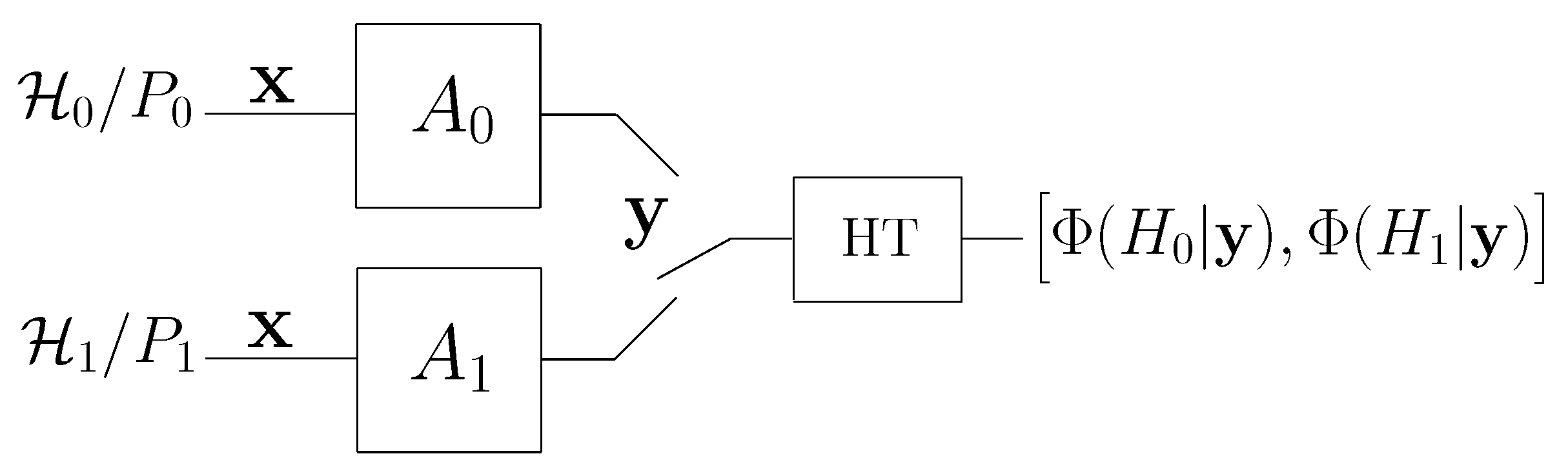
Given two discrete memoryless sources, and , defined over a common finite alphabet , we denote by a sequence emitted by one of these sources. The sequence x is available to the attacker. Let denote the sequence observed by the defender: when an attack occurs under both and , the observed sequence y is obtained as the output of an attack channel fed by x.
In principle, we must distinguish between two cases: in the first, the attacker is aware of the underlying hypothesis (hypothesis-aware attacker), whereas, in the second case, it is not (hypothesis-unaware attacker). In the hypothesis-aware case, the attack strategy is defined by two different conditional probability distributions, i.e., two different attack channels: , applied when holds, and , applied under . Let us denote by the PMF of y under , . The attack induces the following PMFs on y: and .
Clearly, in the hypothesis-unaware case, the attacker will apply the same channel under and , that is, , and we denote the common attack channel simply by A. Throughout the paper, we focus on the hypothesis-aware case as, in view of this formalism, the hypothesis-unaware case is just a special case. Obviously, the partially active case, where no attack occurs under can be seen as a degenerate case of the hypothesis-aware fully active one, where is the identity channel I.
Regarding the defender, we assume a randomized decision strategy, defined by
, which designates the probability of deciding in favor of
,
, given
y. Accordingly, the probability of a
false positive (FP) decision error is given by
and similarly, the
false negative (FN) probability assumes the form:
As in [
11], due to the limited resources assumption, the defender makes a decision based on first-order empirical statistics of
y, which implies that
depends on
y only via its type class
.
Concerning the attack, to limit the amount of distortion, we assume a distortion constraint. In the hypothesis-aware case, we allow the attacker different distortion levels, and , under and , respectively. Then, and , where, for simplicity, we assume that a common (permutation-invariant) distortion function is adopted in both cases.
Figure 1 provides a block diagram of the system with a fully active attacker studied in this paper.
3.2. Definition of the Neyman–Pearson and Bayesian Games
One of the difficulties associated with the fully active setting is that, in the presence of a fully active attacker, both the FP and FN probabilities depend on the attack channels. We therefore consider two different approaches, which lead to different formulations of the detection game: in the first, the detection game is based on the Neyman–Pearson criterion, and, in the second one, the Bayesian approach is adopted.
For the Neyman–Pearson setting, we define the game by assuming that the defender adopts a conservative approach and imposes an FP constraint pertaining to the worst-case attack under .
Definition 1. The Neyman–Pearson detection game is a zero-sum, strategic game defined as follows.
The set of strategies allowed to the defender is the class of randomized decision rules that satisfy
- (i)
depends on y only via its type.
- (ii)
for a prescribed constant , independent of n.
The set of strategies allowed to the attacker is the class of pairs of attack channels such that , ; that is, .
The payoff of the game is ; the attacker is in the quest of maximizing whereas the defender wishes to minimize it.
In the above definition, we require that the FP probability decays exponentially fast with n, with an exponential rate at least as large as . Such a requirement is relatively strong, its main consequence being that the strategy used by the attacker under is irrelevant, in that the payoff is the same whichever is the channel played by the attacker. It is worth observing that, to be more general, we could have defined the problem as a non-zero sum game, where the defender has payoff , whereas for the attacker we consider a payoff function of the form , for some positive constant and . As is made clear in the following section, this non-zero sum version of the game has the same equilibrium strategies of the zero-sum game defined above.
In the case of partially active attack (see the formulation in [
23]), the FP probability does not depend on the attack but on the defender only; accordingly, the constraint imposed by the defender in the above formulation becomes
. Regarding the attacker, we have
, where
is a singleton that contains the identity channel only.
Another version of the detection game is defined by assuming that the defender follows a less conservative approach, that is, the Bayesian approach, and he tries to minimize a particular Bayes risk.
Definition 2. The Bayesian detection game is a zero-sum, strategic game defined as follow.
The set of strategies allowed to the defender is the class of the randomized decision rules where depends on y only via its type.
The set of strategies allowed to the attacker is .
The payoff of the game isfor some constant a, independent of n.
We observe that, in the definition of the payoff, the parameter
a controls the tradeoff between the two terms in the exponential scale; whenever possible, the optimal defense strategy is expected to yield error exponents that differ exactly by
a, so as to balance the contributions of the two terms of Equation (
3).
Notice also that, by defining the payoff as in Equation (
3), we are implicitly considering for the defender only the strategies
such that
. In fact, any strategy that does not satisfy this inequality yields a payoff
that cannot be optimal, as it can be improved by always deciding in favor of
regardless of
y (
).
As in [
11], we focus on the asymptotic behavior of the game as
n tends to infinity. In particular, we are interested in the exponents of the FP and FN probabilities, defined as follows:
We say that a strategy is asymptotically optimal (or dominant) if it is optimal (dominant) with respect to the asymptotic exponential decay rate (or the exponent, for short) of the payoff.
3.3. Asymptotically Dominant and Universal Attack
In this subsection, we characterize an attack channel that, for both games, is asymptotically dominant and universal, in the sense of being independent of the unknown underlying sources. This result paves the way to the solution of the two games.
Let
u denote a generic payoff function of the form
where
and
are given positive constants, possibly dependent on
n.
We notice that the payoff of the Neyman–Pearson and Bayesian games defined in the previous section can be obtained as particular cases: specifically, and for the Neyman–Pearson game and and for the Bayesian one.
Theorem 1. Let denote the reciprocal of the total number of conditional type classes that satisfy the constraint for a given , namely, admissible conditional type classes (from the method of the types, it is known that for any x [19]). Among all pairs of channels , the pair minimizes the asymptotic exponent of u for every and , every and every permutation-invariant .
Proof. We first focus on the attack under and therefore on the FN probability.
Consider an arbitrary channel
. Let
denote a permutation operator that permutes any member of
according to a given permutation matrix and let
Since the distortion function is assumed to be permutation-invariant, the channel
introduces the same distortion as
, and hence it satisfies the distortion constraint. Due to the memorylessness of
and the assumption that
belongs to
(i.e., that
depends on the observed sequence via its type), both
and
are invariant to permutations on
y. Then, we have:
thus
, where we have defined
which also introduces the same distortion as
. Now, notice that this channel assigns the same conditional probability to all sequences in the same conditional type class
. To see why this is true, we observe that any sequence
can be seen as being obtained from
y through the application of a permutation
, which leaves
x unaltered. Then, we have:
Therefore, since the probability assigned by
to the sequences in
is surely less than or equal to 1, we argue that
which implies that,
.
We conclude that minimizes the error exponent of across all channels in and for every , regardless of .
A similar argument applies to the FP probability for the derivation of the optimal channel under
; that is, from the memorylessness of
and the permutation-invariance of
, we have:
for every
. Accordingly,
minimizes the error exponent of
. We then have:
for every
and
. Notice that, since the asymptotic equality is defined in the exponential scale, Equation (
15) holds no matter what the values of
and
are, including values that depend on
n. Hence, the pair of channels
minimizes the asymptotic exponent of
u for any permutation-invariant decision rule
and for any
. ☐
According to Theorem 1, for every zero-sum game with payoff function of the form in Equation (
5), if
is permutation-invariant, the pair of attack channels which is the most favorable to the attacker is
, which does not depend on
. Then, the optimal attack strategy
is
dominant. The intuition behind the attack channel in Equation (
6) is illustrated in
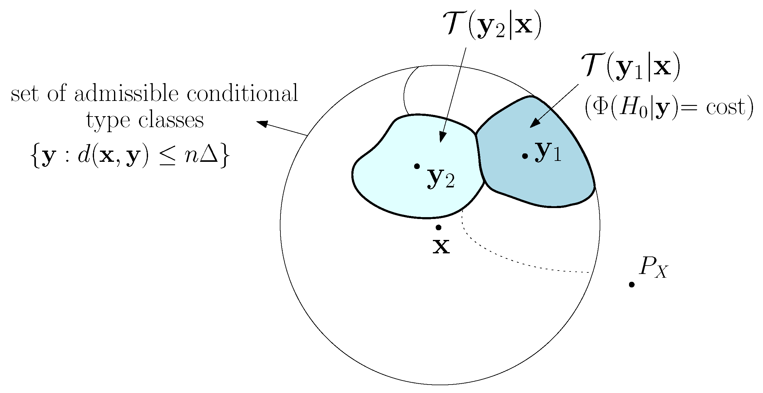
Figure 2 and explained below. Given
x, generated by a source
, the set
corresponds to a set of conditional type classes (for a permutation-invariant distortion function,
is the same for every
). We say that a conditional type class is
admissible if it belongs to this set. Then, to generate
y which causes a detection error with the prescribed maximum allowed distortion, the attacker cannot do any better than randomly selecting an admissible conditional type class according to the uniform distribution and then choosing at random
y within this conditional type class. Since the number of conditional type classes is only polynomial in
n, the random choice of the conditional type class does not affect the exponent of the error probabilities; besides, since the decision is the same for all sequences within the same conditional type class, the choice of
y within that conditional type class is immaterial.
As an additional result, Theorem 1 states that, whenever an adversary aims at maximizing a payoff function of the form Equation (
5), and as long as the defense strategy is confined to the analysis of the first-order statistics, the (asymptotically) optimal attack strategy is
universal with respect to the sources
and
, i.e., it depends neither on
nor on
.
We observe that, if , the optimal attack consists of applying the same channel regardless of the underlying hypothesis and then the optimal attack strategy is fully-universal: the attacker needs to know neither the sources ( and ), nor the underlying hypothesis. In this case, it becomes immaterial whether the attacker is aware or unaware of the true hypothesis. As a consequence of this property, in the hypothesis-unaware case, when the attacker applies the same channel under both hypotheses, subject to a fixed maximum distortion , the optimal channel remains .
According to Theorem 1, for the partially active case, there exists an (asymptotically) dominant and universal attack channel. This result marks a considerable difference with respect to the results of [
11], where the optimal deterministic attack function is found by using the rationalizability argument, that is, by exploiting the existence of a dominant defense strategy, and it is hence neither dominant nor universal.
Finally, we point out that, similar to [
11], although the sources are memoryless and only first-order statistics are used by the defender, the output probability distributions induced by the attack channel
, namely
and
, are not necessarily memoryless.
4. The Neyman–Pearson Detection Game
In this section, we study the detection game with a fully active attacker in the Neyman–Pearson setup as defined in Definition 1. From the analysis of
Section 3.3, we already know that there exists a dominant attack strategy. Regarding the defender, we determine the asymptotically optimal strategy regardless of the dominant pair of attack channels; in particular, as shown in Lemma 1, an asymptotically dominant defense strategy can be derived from a detailed analysis of the FP constraint. Consequently, the Neyman–Pearson detection game has a dominant equilibrium.
4.1. Optimal Detection and Game Equilibrium
The following lemma characterizes the optimal detection strategy in the Neyman–Pearson setting.
Lemma 1. For the Neyman–Pearson game of Definition 1, the defense strategyis asymptotically dominant for the defender. In the special case
,
in Equation (
16) is (asymptotically) equivalent to the Hoeffding test for non-adversarial hypothesis testing [
28].
We point out that, when the attacker is partially active, it is known from [
23] that the optimal defense strategy is
which is in line with the one in [
11] (Lemma 1), where the class of defense strategies is confined to deterministic decision rules.
Intuitively, the extension from Equations (16) and (17) is explained as follows. In the case of fully active attacker, the defender is subject to a constraint on the maximum FP probability over
, that is, the set of the admissible channels
(see Definition 1). From the analysis of
Section 3.3, channel
minimizes the FP exponent over this set. To satisfy the constraint for a given sequence
y, the defender must handle the worst-case value (i.e., the minimum) of
over all the type classes
which satisfy the distortion constraint, or equivalently, all the sequences
x such that
.
According to Lemma 1, the best defense strategy is asymptotically dominant. In addition, since depends on only, and not on , it is referred to as semi-universal.
Concerning the attacker, since the payoff is a special case of Equation (
5) with
and
, the optimal pair of attack channels is given by Theorem 1 and corresponds to
.
The following comment is in order. Since the payoff of the game is defined in terms of the FN probability only, it is independent of . Furthermore, since the defender adopts a conservative approach to guarantee the FP constraint for every , the constraint is satisfied for every and therefore all channel pairs of the form , , are equivalent in terms of the payoff. Accordingly, in the hypothesis-aware case, the attacker can employ any admissible channel under . In the Neyman–Pearson setting, the sole fact that the attacker is active under forces the defender to take countermeasures that make the choice of immaterial.
Due to the existence of dominant strategies for both players, we can immediately state the following theorem.
Theorem 2. Consider the Neyman–Pearson detection game of Definition 1. Let and be the strategies defined in Lemma 1 and Theorem 1, respectively. The profile is an asymptotically dominant equilibrium of the game.
4.2. Payoff at the Equilibrium
In this section, we derive the payoff of the Neyman–Pearson game at the equilibrium of Theorem 2. To do this, we assume an additive distortion function, i.e., . In this case, can be expressed as , where denotes the number of occurrences of the pair in . Therefore, the distortion constraint regarding can be rewritten as . A similar formulation holds for .
Let us define
where
denotes the
empirical expectation, defined as
and the minimization is carried out for a given
. Accordingly, the strategy in Equation (
16) can be rewritten as
When
,
becomes (due to the density of rational numbers on the real line, the admissibility set in Equation (
18) is dense in that of Equation (
21); since the divergence functional is continuous, the sequence
tends to
as
)
where
denotes expectation with respect to
.
The definition in Equation (
21) can be stated for any PMF
in the probability simplex in
. Note that the minimization problem in Equation (
21) has a unique solution as it is a convex program.
The function has an important role in the remaining part of the paper, especially in the characterization of the asymptotic behavior of the games. To draw a parallelism, plays a role similar to that of the Kullback–Leibler divergence in classical detection theory for the non-adversarial case.
The basic properties of the functional are the following: (i) it is continuous in ; and (ii) it has convex level sets, i.e., the set is convex for every . Point (ii) is a consequence of the following property, which is useful for proving some of the results in the sequel (in particular, Theorems 3, 7 and 8).
Property 1. The function is convex in for every fixed P.
The proof follows from the convexity of the divergence functional (see
Appendix A.2).
Using the above definitions, the equilibrium payoff is given by the following theorem:
Theorem 3. Let the Neyman–Pearson detection game be as in Definition 1. Let be the equilibrium profile of Theorem 2. Then, In Equation (
22), we made explicit the dependence on the parameter
in the notation of the error exponent, since this is useful in the sequel.
The proof of Theorem 3, which appears in
Appendix A.3, is based on Sanov’s theorem [
29,
30], by exploiting the compactness of the set
.
From Theorem 3 it follows that whenever there exists a PMF inside the set with -limited expected distortion from . When this condition does not hold, exponentially rapidly.
For a partially active attacker, the error exponent in Equation (
22) becomes
It can be shown that the error exponent in Equation (
23) is the same as the error exponent of Theorem 2 in [
11] (and Theorem 2 in [
31]), where deterministic strategies are considered for both the defender and the attacker. Such equivalence can be explained as follows. As already pointed, the optimal defense strategy in Equation (
17) and the deterministic rule found in [
11] are asymptotically equivalent (see the discussion immediately after Lemma 1). Concerning the attacker, even in the more general setup (with randomized strategies) considered here, an asymptotically optimal attack could be derived as in [
11], that is, by considering the best response to the dominant defense strategy in [
11]. Such attack consists of minimizing the divergence with respect to
, namely
, over all the admissible sequences
, and then is deterministic. Therefore, concerning the partially active case, the asymptotic behavior of the game is equivalent to the one in [
11]. The main difference between the setup in [
11] and the more general one addressed in this paper relies on the
kind of game equilibrium, which is stronger here (namely, a
dominant equilibrium) due to the existence of dominant strategies for both the defender and the attacker, rather than for the defender only.
When the distortion function
d is a metric, we can state the following result, whose proof appears in
Appendix A.4.
Theorem 4. When the distortion function d is a metric, Equation (22) can be rephrased as Comparing Equations (23) and (24) is insightful for understanding the difference between the fully active and partially active cases. Specifically, the FN error exponents of both cases are the same when the distortion under in the partially active case is (instead of ).
When
d is not a metric, Equation (
24) is only an upper bound on
, as can be seen from the proof of Theorem 4. Accordingly, in the general case (
d is not a metric), applying distortion levels
and
to sequences from, respectively,
and
(in the fully active setup) is more favorable to the attacker with respect to applying a distortion
to sequences from
only (in the partially active setup).
6. Source Distinguishability
In this section, we investigate the performance of the Neyman–Pearson and Bayesian games as a function of
and
a, respectively. From the expressions of the equilibrium payoff exponents, it is clear that increase (and then the equilibrium payoffs of the games decrease) as
and
a decrease, respectively. In particular, by letting
and
, we obtain the largest achievable exponents of both games, which correspond to the best achievable performance for the defender. Therefore, we say that two sources are
distinguishable under the Neyman–Pearson (respectively, Bayesian) setting, if there exists a value of
(respectively,
) such that the FP and FN exponents at the equilibrium of the game are simultaneously strictly positive. When such a condition does not hold, we say that the sources are indistinguishable. Specifically, in this section, we characterize, under both the Neyman–Pearson and the Bayesian settings, the
indistinguishability region, defined as the set of the alternative sources that cannot be distinguished from a given source
, given the attack distortion levels
and
. Although each game has a different asymptotic behavior, we show that the indistinguishability regions in the Neyman–Pearson and the Bayesian settings are the same. The study of the distinguishability between the sources under adversarial conditions, performed in this section, in a way extends the Chernoff–Stein lemma [
19] to the adversarial setup (see [
31]).
We start by proving the following result for the Neyman–Pearson game.
Theorem 8. Given two memoryless sources and and distortion levels and , the maximum achievable FN exponent for the Neyman–Pearson game is:where is as in Theorem 3. The theorem is an immediate consequence of the continuity of as , which follows by the continuity of with respect to and the density of the set in as (It holds true from Property 1).
We notice that, if
, there is only an admissible point in the set in Equation (
28), for which
; then,
, which corresponds to the best achievable FN exponent known from the classical literature for the non-adversarial case (Stein lemma [
19] (Theorem 11.8.3)).
Regarding the Bayesian setting, we have the following theorem, the proof of which appears in
Appendix C.1.
Theorem 9. Given two memoryless sources and and distortion levels and , the maximum achievable exponent of the equilibrium Bayes payoff iswhere the inner limit at the left hand side is as defined in Theorem 7. Since
, and similarly
, are convex functions of
, and reach their minimum in
, respectively
(the fact that
(
) is 0 in a
-limited (
-limited) neighborhood of
(
), and not just in
(
), does not affect the argument), the minimum over
of the maximum between these quantities (right-hand side of Equation (
29)) is attained when
, for some PMF
. This resembles the best achievable exponent in the Bayesian probability of error for the non-adversarial case, which is attained when
for some
(see [
19] (Theorem 11.9.1)). In that case, from the expression of the divergence function, such
is found in a closed form and the resulting exponent is equivalent to the Chernoff information (see Section 11.9 [
19]).
From Theorems 8 and 9, it follows that there is no positive
, respectively
a, for which the asymptotic exponent of the equilibrium payoff is strictly positive, if there exists a PMF
such that the following conditions are both satisfied:
In this case, then,
and
are indistinguishable under both the Neyman–Pearson and the Bayesian settings. We observe that the condition
is equivalent to the following:
where the expectation
is with respect to
. For ease of notation, in Equation (
31), we used
(respectively
) as short for
,
(respectively
,
), where
is a joint PMF and
and
are its marginal PMFs.
In computer vision applications, the left-hand side of Equation (
31) is known as the
Earth Mover Distance (EMD) between
and
, which is denoted by
(or, by symmetry,
) [
32]. It is also known as the
-bar distortion measure [
33].
A brief comment concerning the analogy between the minimization in Equation (
31) and
optimal transport theory is worth expounding. The minimization problem in Equation (
31) is known in the Operations Research literature as
Hitchcock Transportation Problem (TP) [
34]. Referring to the original Monge formulation of this problem [
35],
and
can be interpreted as two different ways of piling up a certain amount of soil; then,
denotes the quantity of soil shipped from location (source)
x in
to location (sink)
y in
and
is the cost for shipping a unitary amount of soil from
x to
y. In transport theory terminology,
is referred to as
transportation map. According to this perspective, evaluating the
EMD corresponds to finding the minimal transportation cost of moving a pile of soil into the other. Further insights on this parallel can be found in [
31].
We summarize our findings in the following corollary, which characterizes the conditions for distinguishability under both the Neyman–Pearson and the Bayesian setting.
Corollary 1 (Corollary to Theorems 8 and 9)
. Given a memoryless source and distortion levels and , the set of the PMFs that cannot be distinguished from in both the Neyman–Pearson and Bayesian settings is given by Set is the indistinguishability region. By definition (see the beginning of this section), the PMFs inside are those for which, as a consequence of the attack, the FP and FN probabilities cannot go to zero simultaneously with strictly positive exponents. Clearly, if , that is, in the non-adversarial case, , as any two distinct sources are always distinguishable.
When
d is a metric, for a given
, the computation of the optimal
can be traced back to the computation of the
EMD between
and
P, as stated by the following corollary, whose proof appears in
Appendix C.2.
Corollary 2 (Corollary to Theorems 8 and 9)
. When d is a metric, given the source and distortion levels and , for any fixed P, the minimum in Equation (32) is achieved when Then, the set of PMFs that cannot be distinguished from in the Neyman–Pearson and Bayesian setting is given by According to Corollary 2, when d is a metric, the performance of the game depends only on the sum of distortions, , and it is immaterial how this amount is distributed between the two hypotheses.
In the general case (
d not a metric), the condition on the
EMD stated in Equation (
34) is sufficient in order for
and
P be indistinguishable, that is
(see discussion in
Appendix C.2, at the end of the proof of Corollary 2).
Furthermore, in the case of an distortion function (), i.e., , we have the following corollary.
Corollary 3 (Corollary to Theorems 8 and 9)
. When d is the distortion function, for some , the set Γ can be bounded as follows Corollary 3 can be proven by exploiting the Hölder inequality [
36] (see
Appendix C.3).
7. Concluding Remarks
We consider the problem of binary hypothesis testing when an attacker is active under both hypotheses, and then an attack is carried out aiming at both false negative and false positive errors. By modeling the defender–attacker interaction as a game, we defined and solved two different detection games: the Neyman–Pearson and the Bayesian game. This paper extends the analysis in [
11], where the attacker is active under the alternative hypothesis only. Another aspect of greater generality is that here both players are allowed to use randomized strategies. By relying on the method of types, the main result of this paper is the existence of an attack strategy, which is both
dominant and
universal, that is, optimal regardless of the statistics of the sources. The optimal attack strategy is also independent of the underlying hypothesis, namely
fully-universal, when the distortion introduced by the attacker in the two cases is the same. From the analysis of the asymptotic behavior of the equilibrium payoff, we are able to establish conditions under which the sources can be reliably distinguished in the fully active adversarial setup. The theory developed permits to assess the security of the detection in adversarial setting and give insights on how the detector should be designed in such a way to make the attack hard.
Among the possible directions for future work, we mention the extension to continuous alphabets, which calls for an extension of the method of types to this case, or to more realistic models of finite alphabet sources, still amenable to analysis, such as Markov sources. As mentioned in the Introduction, it would be also relevant to extend the analysis to higher order statistics. In fact, the techniques introduced in this paper are very general and lend themselves to extensions that allow richer sets of sufficient statistics (as currently pursued in an ongoing work of the first two coauthors). This generalization, however, comes at the price of an increased complexity of the analysis with regard to both the expressions of the equilibrium strategies and the performance achieved by the two parties at the equilibrium. More specifically, given the set of statistics used by the defender, it turns out that the optimal attacker also uses the very same statistics (plus the empirical correlation with the source sequence, due to the distortion constraint) and the optimal attack channel is given in terms of uniform distributions across conditional types that depend on these set of statistics. Therefore, in a sequence of games, where the defender exploits more and more statistics, so would the attacker, and it would be interesting to explore the limiting behaviour of this process.
We also mention the case of unknown sources, where the source statistics are estimated from training data, possibly corrupted by the attacker. In this scenario, the detection game has been studied for a partially active case, with both uncorrupted and corrupted training data [
13,
14]. The extension of such analyses to the fully active scenario represents a further interesting direction for future research.
Finally, we stress that, in this paper, as well as in virtually all prior works using game theory to model the interplay between the attacker and the defender, it is assumed that the attacker is always present. This is a pessimistic or worst-case assumption, leading to the adoption of an overly conservative defense strategy (when the attacker is not present, in fact, better performance could be in principle achieved by adopting a non-adversarial detection strategy). A more far-reaching extension would require that the ubiquitous presence of the attacker is reconsidered, for instance by resorting to a two-steps analysis, where the presence or absence of the attacker is established in the first step, or by defining and studying more complex game models, e.g., games with incomplete information [
37].


